
Submitted:
29 August 2025
Posted:
01 September 2025
You are already at the latest version
Abstract
Developing classical three-dimensional consolidation theories considers the small-strain assumption. This small-strain assumption is inappropriate when studying the consolidation process of soft or very soft clay layers. Instead, this study derives a generalized mathematical model describing a three-dimensional finite-strain consolidation process and applies the deep Galerkin method to deduce its numerical solution. Developing this mathematical model uses the Reynolds transport theorem to describe mass and momentum balances for clay grain and pore water phases. The governing equation is the sum of the resulting mass and momentum balance equations. Next, the deep Galerkin method is applied to train a deep neural network to minimize the loss function defined by the governing equation and available initial and boundary conditions. The unknowns are the average velocity, effective stress, and pore water pressure. Predicting consolidation settlements is implemented by updating the problem domain using the resulting average velocity. Beneficial from the deep Galerkin method, two real-world examples demonstrate that the current mathematical model provides accurate predictions of consolidation settlements caused by the self-weight of two very soft clay layers. The deep Galerkin method helps eliminate the need to specify complete boundary conditions, which is difficult to achieve in modeling a finite strain consolidation process.
Keywords:
finite strain consolidation
; Reynolds transport theorem
; deep Galerkin method
; mass and moment balance equations
; self-weight
1. Introduction
Consolidation represents the time-dependent process by which clay decreases its volume due to the expulsion of pore water under an external loading or its self-weight. A consolidation theory or a mathematical model describing the consolidation process is essential in many actual problems such as estimating the consolidation settlements due to a construction loading (e.g., [1]), evaluating the results of a sand drain scheme (e.g., [2]), and scheduling a land reclamation project (e.g., [3]). Unexpected consolidation settlements may damage a building and delay a land reclamation project.
Nevertheless, developing classical mathematical models describing consolidation processes considers the small-strain assumption (e.g., [4]) in which consolidation settlements do not substantially change the thickness of a clay layer. It is invalid for a soft or very soft clay layer since it may be significantly thinner due to its consolidation settlements. These consolidation settlements may be caused only by their self-weight. A real example may be the Kansai airport, which may gradually sink into the sea due to excessive settlements of undersea clay layers. However, we only had one-dimensional [5,6] or quasi multi-dimensional mathematical models [7] to describe the consolidation process of a soft or very soft clay layer. Developing these mathematical models assumes that a soft or very soft clay layer deforms only in the vertical direction. This assumption is inconsistent with the actual condition.
Therefore, the author’s thesis [8] developed a generalized mathematical model describing a generalized finite-strain consolidation process. The Reynolds transport theorem [9] is employed to represent mass and momentum balances. The previous thesis [8] further combined the resulting mass and momentum equations into one single governing equation. Nevertheless, the resulting governing equation is long and complex. Applying it to model a real problem is difficult since we have few numerical methods to solve it. To solve this drawback, this study applies the deep Galerkin method (DGM) [10] to minimize the loss function defined by the sum of resulting momentum equations, initial, and boundary conditions. The unknowns are the average velocity field, effective stress, and pore water pressure. Calculating consolidation settlements is implemented by updating the problem domain according to the resulting average velocity field.
This DGM (e.g., [10]) is a meshless deep algorithm for solving high-dimensional partial differential equations. Choosing it considers the difficulties of collecting necessary data to define the boundary conditions (for example, a deep boundary) of a soft or very soft clay layer. By using the DGM, we train a deep neural network to provide a solution to a partial differential equation at random points in a problem domain. Defining complete boundary conditions is unnecessary.
The objectives of creating this study are
- Compensate for the absence of a useful mathematical model for describing a generalized finite-strain consolidation process. It advances the simulation of the finite-strain consolidation process of soft or very soft clay layers. Compared to traditional small-strain consolidation theories (e.g., [4]), the proposed mathematical model has more applications, such as estimating settlements of dredge fill deposits.
- Extend the application of the DGM to a partial differential equation with a problem domain subjected to large strains.
The remainder of this article has four sections. Section 2 presents a review of published articles relevant to this study. Section 3 presents the development of a generalized finite strain consolidation theory and its DGM solution. Section 4 presents the numerical results generated using the current mathematical model. Comparing these numerical results to observed settlements of the phosphatic waste clay and Osaka Bay mud is done in this section. Based on this comparison, Section 5 presents a discussion. Section 6 presents conclusions and the concluding remark of this research.
2. Related Works
This study intends to develop a mathematical model to describe a generalized finite-strain consolidation process and apply the DGM to solve the unknowns. Therefore, relevant references are those articles presenting a two- or three-dimensional finite strain consolidation theory and applications of the DGM to solve various partial differential equations.
2.1. Finite Strain Consolidation Theory
When we intend to develop a generalized finite strain consolidation theory, the origin is usually the one-dimensional finite strain consolidation theory proposed by Gibson et al. [5,6]. Different from Biot [4], they used the void ratio as the main unknown of their mathematical model. Considering that consolidation settlements may substantially thin a soft clay layer, they defined a convective coordinate system to describe the changes in a clay layer’s thickness. Besides, Gibson et al. [5,6] accounted for the effects of a thick clay layer’s self-weight on its consolidation process.
After the one-dimensional finite strain consolidation theory [5,6], few articles presented a truly generalized finite strain consolidation theory. However, quasi-two- or three-dimensional theories are available. For example, Jeeravipoolvarn et al. [7] developed a quasi-three-dimensional finite strain consolidation theory, which assumed that pore water flows in any direction and pore pressure dissipation causes only vertical deformations. Huerta and Rodriguez (1992) [11] calculated finite-strain consolidation settlements of soft sediment fillings at high water levels. They considered one-dimensional deformations and two-dimensional fluxes. Liu et al. (2021) [12] assumed vertical strains. They evaluated the vertical drains combined with vacuum pressure using a quasi-axisymmetric finite strain consolidation theory.
The author’s Ph.D. thesis [8] presented a truly three-dimensional finite strain consolidation theory. This generalized finite strain consolidation theory extended the one-dimensional works provided by Gibson et al. [5,6]. Creating this extension used the Reynolds transport theory to model the mass and momentum balances for the clay grain and pore water phases. Limiting the deformation and pore water dissipation in the vertical direction is not required. Besides, the effect of the self-weight of a thick clay layer on its consolidation process is studied. However, the resulting mathematical model may be complex.
2.2. Deep Galerkin Method
Since this study chooses the DGM (e.g., [10]) to solve the proposed mathematical model, it is necessary to review the representative partial differential equations, which were solved using the DGM:
Kumar et al. (2022) [13] used the DGM to solve the one-dimensional Burger-Huxley and Huxley equations. They are second-order partial differential equations with initial and boundary conditions. In the application of DGM, estimating the time derivatives using a finite difference scheme was not required. Approximating a time derivative by a finite difference scheme is frequently seen in the application of the finite element method in solving a time-dependent partial differential equation.
Sirignano and Spiliopoulos (2018) [10] applied the DGM to a free boundary equation. It is a one-dimensional and second-order partial differential equation. Its theoretical background is the stock price dynamics. One of the boundaries is a time-dependent function. It enters into the derivation of the loss function defined to implement the DGM.
Masaharu (2021) [14] employed the DGM to solve a compressible Navier-Stokes equation. The Navier-Stokes equation contains convective accelerations. They are highly nonlinear differential terms. We may notice that Masaharu (2021) [14] studied supersonic flows around a blunt body without specifying full boundary conditions. This example is quite different from the application of a finite element method.
3. Generalized Finite Strain Consolidation
3.1. Mathematical Model
Suppose a homogeneous and saturated soil layer. Besides, clay grains and pore water are incompressible. The convective coordinate is defined to identify a point in a problem domain .
If denotes the total amount of an extensive property within , the Reynolds transport theorem states that the conservation of can be represented by [9]
where is the total derivative with respect to the time t, is the density of , V is the volume of , S is the boundary of , the subscript S denotes the boundary, · is the dot operator, is the velocity field, and is an unit vector normal to S.
3.1.1. Mass Balance for the Clay Grain Phase
Substituting into Equation (1) results in
where f is a function, the subscript S denotes the clay grain phase, n is the porosity, is the density. Applying the definition of total derivative and coordinate transform to simplify Equation (2) yields
in which the subscript 0 denotes the Lagrangian coordinate , ∇ is the gradient vector, is the Jacobian, are the components of convective coordinate , and are the components of Lagrangian coordinate .
Applying the Gauss theorem and coordinate transform to simplify the final term of Equation (3) yields
Combining the final term of Equation (4) with the eight term in Equation (3) yields . Substituting the resulting expression into Equation (3) yields
Or we can consider the localization and write
3.1.2. Mass Balance for the Pore Water Phase
Considering the localization to simplify Equation (11) yields
Equation (12) is the mass balance equation for the pore water phase.
3.1.3. Momentum Balance for the Clay Grain Phase
Substituting into Equation (1) yields
By simplifying Equation (14) using the Gauss theorem and transforming the final term of the same equation using the coordinate transformation, we can reduce the equation to
Combining the final two terms of Equation (15) yields
Based on Equation (6), Equation (16) is equal to 0. We then simplify Equation (13) to
where the term is the acceleration field and denotes the mass of clay grains (in ). Therefore, this equation is equal to the forces exerted on clay grains. Thus, we can define:
in which denotes the stress tensor, the prime represents the effective stress, is the seepage force vector per unit volume arising from the frictional drag of pore water, and is the body force vector. This study considers that the comes from the weights of clay grains. It and can be further equated by
where and g is the gravity acceleration. The sign ± depends upon the direction of . If the direction of is opposite to the direction of the gravitational force, the sign + is adopted. Meanwhile, applying the Gauss theorem to simplify the final term of Equation (18) yields . Substituting the resulting expression into Equation (18). Considering Equation (17) and the localization, we can deduce:
Equation (20) is the momentum balance equation for the clay grain phase.
3.1.4. Momentum Balance for the Pore Water Phase
Substituting into Equation (1) yields
Referring to the derivation of Equation (14) to simplify the first term of Equation (21) and applying the Gauss theorem and coordinate transform to the final term of the same equation, the resulting equation is
The final two terms of Equation (22) are combined and reduced to
Similar to Equation (17), Equation (24) is equal to the forces exerted on the pore water phase. Thus [9]
where denotes the pore water pressure tensor, is the reactive force vector per unit volume exerted by clay grains on the pore water phase as the pore water seeps through the clay, and is the body force vector. The and are further defined by
in which p is the pore water pressure and setting the sign ± still depends upon the direction of . On the other hand, applying the Gauss theorem to the final term of Equation (25) yields . Substituting the resulting expression into Equation (25) and considering the localization, we can obtain:
Equation (27) is the momentum balance equation for the pore water phase.
3.2. DGM Formulation
Summing Equations (20) and (27) results in
where denotes the average velocity field, represents the average acceleration field, and is the total mass density. Different from the author’s thesis [8], this study does not try to combine Equations (9), (12), (20), and (27) into a governing equation. Thus, deriving a DGM solution of the current mathematical model is simpler.
Furthermore, assume [8] or neglects the interaction between pore water and clay grains. Simplifying Equation (28) with this consideration yields
A DGM solution of Equation (29) is next derived: Suppose the time t is between 0 and T. The initial and boundary conditions are
where , , , and are free, drained, fixed, and undrained boundaries, respectively, is the initial pore water pressure tensor, represents the initial effective stress tensor, denotes an imposed loading, and is the component of a unit vector normal to the undrained boundary . Note that , , , and may not exist simultaneously in a particular problem domain . Also the computation of and depends upon a particular problem domain .
Based on Equations (29)-(34), this study applied the DGM algorithm to approximate the using , using , and using in which is the neural network’s parameter. The DGM algorithm defines the loss function by (e.g., [10])
where is the component of the tensor, the symbol represents the norm function in which measures how well the functions , , and satisfy Equations (29)-(34). If we can obtain , the , , and are the solutions of Equation (29).
The goal of defining Equation (35) is to find the parameter with which the corresponding , , and minimize the function. Then, they are solutions of the , , and . The best value is estimated using an existing optimization method (for example, the Adam optimizer). Discretizing the problem domain into some elements is unnecessary.
Algorithm 1 [14] illustrates the proposed steps of implementing the DGM algorithm and three post-processing steps (6th-8th steps) in which k denotes an iteration number, E denotes an error, represents the learning rate, and is the compliance matrix, R denotes the void ratio-effective stress relationship, and is the strain tensor. The sixth step provides the strain tensor or void ratio e. The seventh step outputs the numerical results for updating the Jacobian J and . Since the initial displacement and velocity fields are zero, the eighth step is employed to update the coordinates . Updating the coordinates also provides the consolidation settlements. Note that this study does not calculate consolidation settlements from the strain tensor since collecting undisturbed samples of soft or very soft clay to construct its stress-strain and void ratio-stress relationships is difficult.
| Algorithm 1 DGM algorithm |
|
The learning rate in Algorithm 1 decreases with the iteration number k. The calculation is unbiased estimation of :
where denotes the mathematical expectation. Under technical conditions, the parameter will converge to a critical point of the function as :
Figure 1 (e.g., [13,14]) shows an example of the neural network’s architecture for implementing the DGM. It approximates the by , by , and by in which is the neural network’s parameter. In mathematical expressions, the deep neural network contains three types of layers:
- Input layer: The neural network calculates:in which , is the intermediate hidden feature vector, represents the activation function, denotes the input weight matrix, and represents the input bias vector.
- Hidden layer: Suppose L hidden layers are generated. For each hidden layer, the neural network computes:where denotes the L-th hidden layer, is the gate vector, the subscripts f, r, and h denote the update gate, reset gate, and candidate hidden gate; respectively, represents the reset gate. represents the candidate hidden state, ⊙ is the Hadamard product, and tanh is the hyperbolic tangent function. This tanh function serves as a nonlinear activation function.
- Output layer:where represents the output of the neural network, is the weight matrix of the output layer, and is the bias vector of the output layer.
3.3. Implementation of the DGM
This study uses PyTorch in coding a Python program for implementing Algorithm 1. It has an automatic differentiation function that can easily output the derivatives with respect to independent variables. Moreover, back propagation is adopted to train a deep neural network. Besides, optimizing the training process adopts the Adam optimizer based on the stochastic gradient descent method. Furthermore, a Mac Pro is employed to generate numerical results. Since it has 16 GPUs, the total time of implementing Algorithm 1 can be limited to about 10 minutes.
4. Application
Considering the acquisition of experimental data, this study introduces the recorded consolidation settlements of the phosphatic waste clay [15] and Osaka Bay [16] mud to test Algorithm 1.
4.1. Phosphatic Waste Clay
The phosphate waste clay is the by-product of the beneficiation process of the phosphate ore. This phosphate ore occurs in a gravely, clayey sand and contains phosphate, granular materials (sand), and clays. Merely the phosphate is collected as the primary source of phosphorus in inorganic fertilizers. After extracting the phosphate, the phosphate waste clay is pumped into large retention ponds and allowed to consolidate without any imposed loading. For designing the storage capacity of the retention ponds, we must predict well the consolidation settlements of the phosphate waste clay caused by its self-weight.
The phosphate waste clay has a liquid limit between 100 and 200, a plastic index between 70 and 150, and a specific yield equal to 2.71 [15]. Some previous studies have constructed empirical relationships between the void ratio and effective stress. Equation (41) provides an example [17]:
where and are the anticipated void ratios before and after the consolidation process, and is an empirical parameter. This word ’anticipated’ denotes the difficulty of measuring the void ratio within the whole phosphate waste clay layer.
Testing the performance of the current mathematical model is through the results of a field test [17]. In this field test, a retention pond settled due to the self-weight of poured phosphate waste clay. Cargill [3] derived a one-dimensional mathematical model to predict the consolidation settlements. Instead, this study applied the two-dimensional version of the proposed mathematical model to predict the consolidation settlements and compare the measured results. The initial problem domain is () in which H is the depth of the retention pond, the direction of is identical to the direction of the gravitational force, and the is from right to left. A small figure inside the subsequent Figure 2 also illustrates the initial problem domain. The two-dimensional version of Equation (29) is the governing equation:
The initial and boundary conditions are
where is the unit weight of pore water. Moreover, the previous study [17] provided the following data:
in which the high ratio value implies that the phosphate waste clay layer is very soft. Meanwhile, training a deep neural network uses the Adam optimizer, learning rate equal to , and epochs. This deep neural network has two hidden layers, and each hidden layer has 128 neurons. Discretizing the problem domain and uses interior nodes and boundary nodes.
After subtracting predicted consolidation settlements from the elevation of the retention pond, Figure 2 compares the remaining elevation. Figure 3(a)-Figure 3(d) selectively show the predicted , , , and at the time t = 30 days. The unit of predicted , , , and is .
Figure 2 shows the necessity of developing a general mathematical model for studying a finite strain consolidation process. Considering the horizontal pore water dissipation, the current mathematical model provides more accurate predicted elevations of the retention pond, especially during 10-100 days. The corresponding maximum error is about 2.3%, whereas the previous one-dimensional model [17] outputs the maximum error about 4.2 %. Figure 3(a) and Figure 3(b) show that the and vary symmetrically to two skewed vertical axes. Besides, Figure 3(c) demonstrates that a nonuniform exerts on the retention pond. It is impossible to use a one-dimensional mathematical model to output variations of the , , and shown in Figure 3(a)-Figure 3(c). Meanwhile, Figure 3(d) demonstrates that the pore water pressure varies uniformly across the depth of the retention pond.
Figure 4 demonstrates the convergence of the value with respect to the number of epochs. This figure indicates that the value decreases to a low value after running Algorithm 1 sufficiently.
If we desire the values below , Figure 4 indicates that we can adopt merely 4000 to 5000 epochs to generate such predictions. However, it may be interesting to study how to investigate the variation of values with respect to the learning rate and the number of interior or boundary nodes
4.2. Osaka Bay Mud
Since Japan has limited land and a dense population, it has no choice but to build some offshore public facilities. Therefore, some published studies (e.g., [16]) investigated the consolidation behaviors of offshore clay layers near big cities such as Tokyo and Osaka. This study uses the results of a model test [16] whose goal is to monitor the consolidation process induced by the self-weight of an Osaka Bay mud layer to test the current mathematical model.
The previous study [16] reported that Osaka Bay mud has a liquid limit equal to 102.8, a plastic index identical to 45.8, and a specific yield equal to 2.59. Another published study [18] provided an empirical relationship between the void ratio and vertical effective stress :
Similar to Section 4.1, Equation (42) is still the governing equation for predicting consolidation settlements of the Osaka Bay mud layer with setting the initial problem domain identical to () in which H is the thickness of the Osaka Bay mud layer. The direction of is identical to the direction of the gravitational force, whereas the direction of is from left to right. The small figure inside the subsequent Figure 5 further illustrates this problem domain . The initial and boundary conditions are
Other necessary data are [16]:
in which the initial void ratio indicates that the Osaka mud layer is softer than the phosphate waste clay layer in Section 4.1. Meanwhile, training a deep neural network uses the Adam optimizer, learning rate equal to , and epochs. This deep neural network has two hidden layers, and each hidden layer has 128 neurons. Discretizing the problem domain and uses interior nodes and boundary nodes. Figure 5 compares the predicted and measured vertical settlements. Figure 6(a)-Figure 6(d) selectively show variations of the predicted , , , and at the time t = mins.
Figure 5 indicates that the current mathematical model provides accurate predictions of vertical settlements. Further inspection of the data used to plot this figure finds that the maximum error is below 5%. Although the Osaka Bay mud layer in this section is thinner than the phosphate waste clay layer in Section 4.1, Figure 6(a) still shows that nonuniform imposes the Osaka Bay mud layer. Larger stresses are imposed on the middle part of the Osaka Bay mud layer. Similarly, Figure 6(c) demonstrates that the shear stress varies non-uniformly. In contrast, Figure 6(b) and Figure 6(d) shows that variations of the and are uniform.
Figure 7 visualizes the convergence of the value with respect to the number of epochs. Similar to Section 4.1, if the desired value is below , this figure shows that we can adopt merely 2000 epochs to obtain such values. Convergence of the value is even faster in this section than in Section 4.1, although more complex boundary conditions are in this section.
4.3. Ablation Study
In Section 3.2, Equation (32) defines the value. Several parameters can affect its convergence. Compared to the error analysis in the application of other numerical methods (for example, the finite element method) to solve a partial differential equation, this study chooses to inspect the value with respect to different learning rates and numbers of interior and boundary nodes. Obviously, increasing the number of hidden layers or neurons can provide lower values. Discussing the influence of the number of hidden layers or neurons on the value can’t deliver new results.
Figure 8(a)-Figure 8(b) compare the values with respect to the learning rates and . Except for the learning rate , creating Figure 8(a) uses the required data or settings for plotting Figure 2, Figure 3(a)-Figure 3(d), and Figure 4, whereas generating Figure 8(b) employs the required data or settings for drawing Figure 5, Figure 6(a)-Figure 6(d), and Figure 7.
Observing Figure 8(a)-Figure 8(b), one may find that training the deep neural network using the faster learning rate is not appropriate. The corresponding value does not converge to an acceptable value (below ) in Figure 8(a). In contrast, the value is below when training the deep neural network over 4000 to 5000 epochs with the learning rate .
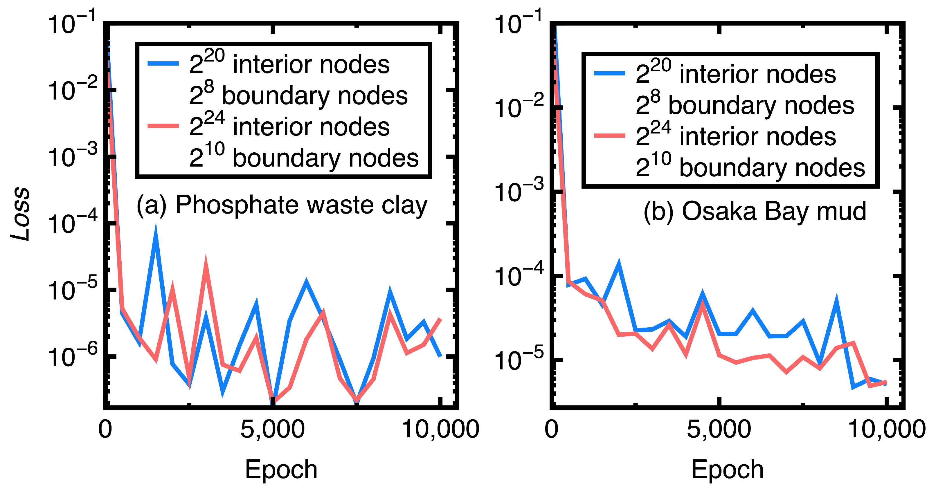
Figure 9(a)-Figure 9(b) compare the values versus different numbers of interior and boundary nodes. Except for the number of interior or boundary nodes, editing Figure 9(a) uses the data and settings required to prepare Section 4.1m while creating Figure 9(b) is based on the necessary data and settings employed to generate Figure 5, Figure 6(a)-Figure 6(d), and Figure 7. For keeping a particular nodal spacing, the total number of interior and boundary nodes is simultaneously increased in creating Figure 9(a)-Figure 9(b).
Increasing the total number of interior and boundary nodes means a finer discretization of the problem domain. Since this study creates random interior and boundary nodes, Figure 9(a)-Figure 9(b) indicate that generating a finer discretization of the problem domain does not apparently improve the value. These two figures may show a distinguishing characteristic, which does not exist in other existing numerical methods (for example, the finite element method). A finer discretization of the problem domain can apparently improve the accuracy of numerical results.
5. Discussion
Section 4.1 and Section 4.2 reveal four difficulties of developing a mathematical model for an engineering problem; however, this study resolves these difficulties to a certain extent:
- The first difficulty is the challenge of balancing the number of assumptions and the simplicity of the corresponding governing equations. This study eliminates the assumption that a clay layer consolidates only in the vertical direction in modeling a finite strain consolidation process; however, the current governing equation (Equation (29)) is not complex.
- The second difficulty is the harassment of choosing a suitable numerical method for solving a real-world problem. For this study, it is difficult to define some boundary conditions of a natural soft clay layer; nevertheless, boundary conditions are prerequisites for implementing existing numerical methods (for example, the finite element method). Section 4.1 provides an example. Probably due to the lack of field measurements, some boundary conditions were unavailable in the previous study [17]. However, the DGM can resolve this difficulty since its goal is to minimize the value at random nodes.
- The third difficulty is the requirement that the total number of governing equations equals the total number of unknowns. The DGM helps eliminate this requirement. In Section 4.1 and Section 4.2, two governing equations are available, but six unknowns (pore water pressure, two average velocity components, and three effective stress components) exist. If this study does not adopt the DGM, reducing the total number of unknowns must be implemented using available material properties (for example, a void ratio-stress relationship). The author’s Ph.D. thesis provided an example in which the void ratio is the unknown of a single and complex governing equation.
- The fourth difficulty is the non-homogeneity of clay’s properties. This difficulty represents the limitation of this study. Natural clay’s properties are non-homogeneous. Although we can create a particular probability model to regress the distribution of a clay’s property, there must be enough clay samples to provide accurate regression points. However, gathering clay samples of a natural soft clay layer is not easy. Probably due to this reason, it is unavoidable that the accuracy of predicted consolidation settlements is limited.
Meanwhile, Section 4.3 demonstrates that the DGM may be a promising numerical method for studying engineering problems. Even in a finite-strain engineering problem, we only need to adjust the learning rate in implementing a particular deep neural network.
6. Conclusions and Concluding Remark
This study develops a mathematical model for describing a generalized finite strain consolidation process and its DGM solution. Developing this mathematical model adopts the Reynolds transport theorem to describe mass and momentum balances for clay grain and pore water phases. The governing equation is the sum of the resulting mass and momentum balance equations. Applying the DGM to train a deep neural network to minimize a loss function defined using the resulting governing equation, available initial, and boundary conditions, is next implemented. Two real-world problems show that the current mathematical model outperforms previous one-dimensional models in predicting the consolidation settlements caused by the self-weights of two natural soft clay layers. Besides, an additional ablation study finds that the learning rate has an apparent effect on the value of the loss function.
Based on Section 4.1-Section 4.3, the conclusions of this study are
- Deriving the current mathematical model advances the modeling of a finite-strain engineering problem. The current governing equation is simple but adapts to the changes of the problem domain. Based on it, we can predict more accurate settlements.
- The DGM is a promising numerical method for resolving the difficulties of deducing sufficient governing equations or specifying full initial and boundary conditions in solving a partial differential equation.
- To obtain the desired accuracy of numerical results provided by the DGM, adopting a lower learning rate in training a deep neural network is preferred.
Furthermore, the limitation of this study is the non-homogeneity of clay properties. Since implementing the DGM uses random interior and boundary nodes, constructing particular probability models to regress the distributions of clay properties and combining the resulting probability model with a DGM solution may be the main interest of future research.
Funding
This research is the author’s private work and received no external funding.
Data Availability Statement
Data used to implement Section 4.1 and Section 4.2 are digitized from two previous studies [16,17]. They are available on https://github.com/xsheu/consolidation.
Acknowledgments
The author completed this article without any financial support.
Conflicts of Interest
The authors declare no conflicts of interest.
Abbreviations
The following abbreviations are used in this manuscript:
| DGM | Deep Galerkin Method |
References
- Loktev, K.A.; Ulanov, I.; Shishkina, I.; Savulidi, M.; Klekovkina, N.; Kuznetsov, A. Determination of settlement parameters of highway embankment and base consolidation time depending on soil characteristics. Transp. Res. Proc. 2022, 63, 946–955. [CrossRef]
- Kamash, W.E.; Hafez, K.; Zakaria, M.; Moubarak, A. Improvement of soft organic clay soil using vertical drains. KSCE. J. Civ. Eng. 2021, 25(2), 429–441. [CrossRef]
- Cao, L.F.; Chang, M.-F.; Teh, C.I. and Na, Y.M. Back-calculation of consolidation parameters from field measurements at a reclamation site. Can. Geotech. J. 2001, 38(4), 755–769. [CrossRef]
- Biot, M.A. General theory of three-dimensional consolidation. J. Appl. Phys. 1941, 12(2), 155–164. [CrossRef]
- Gibson, R.E.; England, G.L.; Hussey, M.J.L. The theory of one-dimensional consolidation of saturated clays. Géotechnique 1967, 17(3), 261–273.
- Gibson, R.E.; Schiffman, R.L.; Cargill, K.W. Back-calculation of consolidation parameters from field measurements at a reclamation site. Can. Geotech. J. 2001, 38(4), 755–769. [CrossRef]
- Jeeravipoolvarn, S.; Scott J.D.; Chalaturnyk R. Multi-dimensional finite strain consolidation theory: Modeling study. In Proceedings of the 61st Canadian Geotechnical Conference and the 9th Joint CGS/IAH-CNC Groundwater Conference, Edmonton, AB, Canada, September 21-24, 2008; 167–175.
- Sheu, G.Y. A general finite strain consolidation theory. Ph.D. Thesis, National Cheung Kung University, Tainan, Taiwan, 1997.6.30.
- Malvern, L.E. Introduction to the Mechanics of a Continuous Medium, Prentice-Hall: Englewood Cliffs, New Jersey, USA, 1977.
- Justin S.; Konstantinos S.: DGM: A deep learning algorithm for solving partial differential equations. J. Comput. Phys. 2018, 375, 1339–1364.
- Huerta, A.; Rodriguez, A.: Numerical analysis of nonlinear large-strain consolidation and filling. Degree-Comput. Struct. 1992, 44(1), 357–365.
- Liu, S.J.; Sun, H.L.; Pan, X.D.; Shi, L.; Cai, Y.Q.; Geng, X.Y.: Analytical solutions and simplified design method for large-strain radial consolidation. Comput. Geotech. 2021, 134, 103987. [CrossRef]
- Kumar, H.; Yadav, N.; Nagar, A.K.: Numerical solution of Generalized Burger-Huxley & Huxley’s equation using deep Galerkin neural network method. Eng. Appl. Artif. Intell. 2022, 115, 105289.
- Matsumoto, M.: Application of deep Galerkin method to solve compressible Navier-Stokes equations. Trans. Jpn. Soc. Aeronaut. Space Sci. 2021, 64(6), 348–357. [CrossRef]
- McVay, M.; Townsend, F.; Bloomquist, D.: Quiescent consolidation of phosphatic waste clays. J. Geotech. Eng. 1986, 112(11), 1033–1049. [CrossRef]
- Zen, K.; Umehara, Y. (2019). A new consolidation testing procedure and technique for very soft soils. In Consolidation of Soils: Testing and Evaluation; R. N. Yong; F. C. Townsend, Eds.; American Society for Testing and Materials: Philadelphia, USA; pp. 405–432.
- Cargill, K. W.: Prediction of consolidation of very soft soil. J. Geotech. Eng. 1984, 110(6), 775–795. [CrossRef]
- Hiroyuki T.; Jacques L.: A microstructural investigation of Osaka Bay clay: the impact of microfossils on its mechanical behaviour. Can. Geotech. J. 1999, 36(3), 493–508.
Figure 1.
An example for the neural network’s architecture for implementing the DGM (e.g., [10])
Figure 1.
An example for the neural network’s architecture for implementing the DGM (e.g., [10])
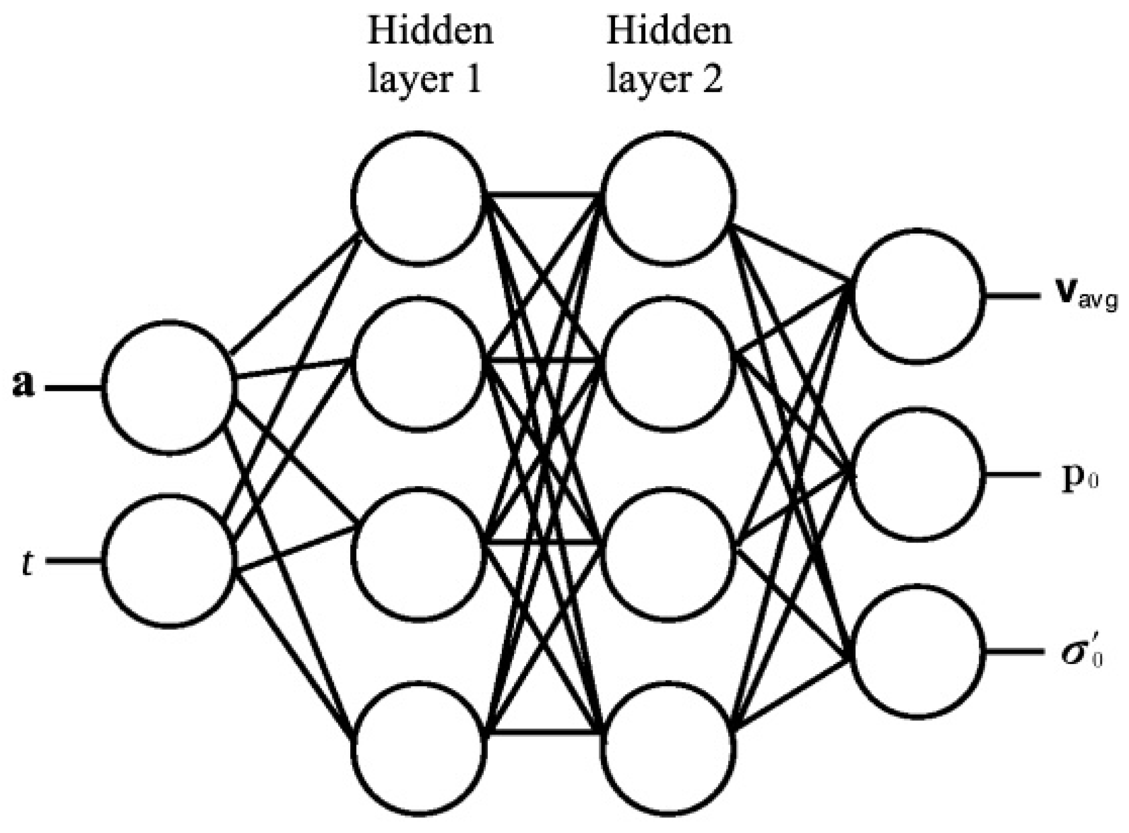
Figure 2.
Comparison of the predicted and observed elevations of the retention pond
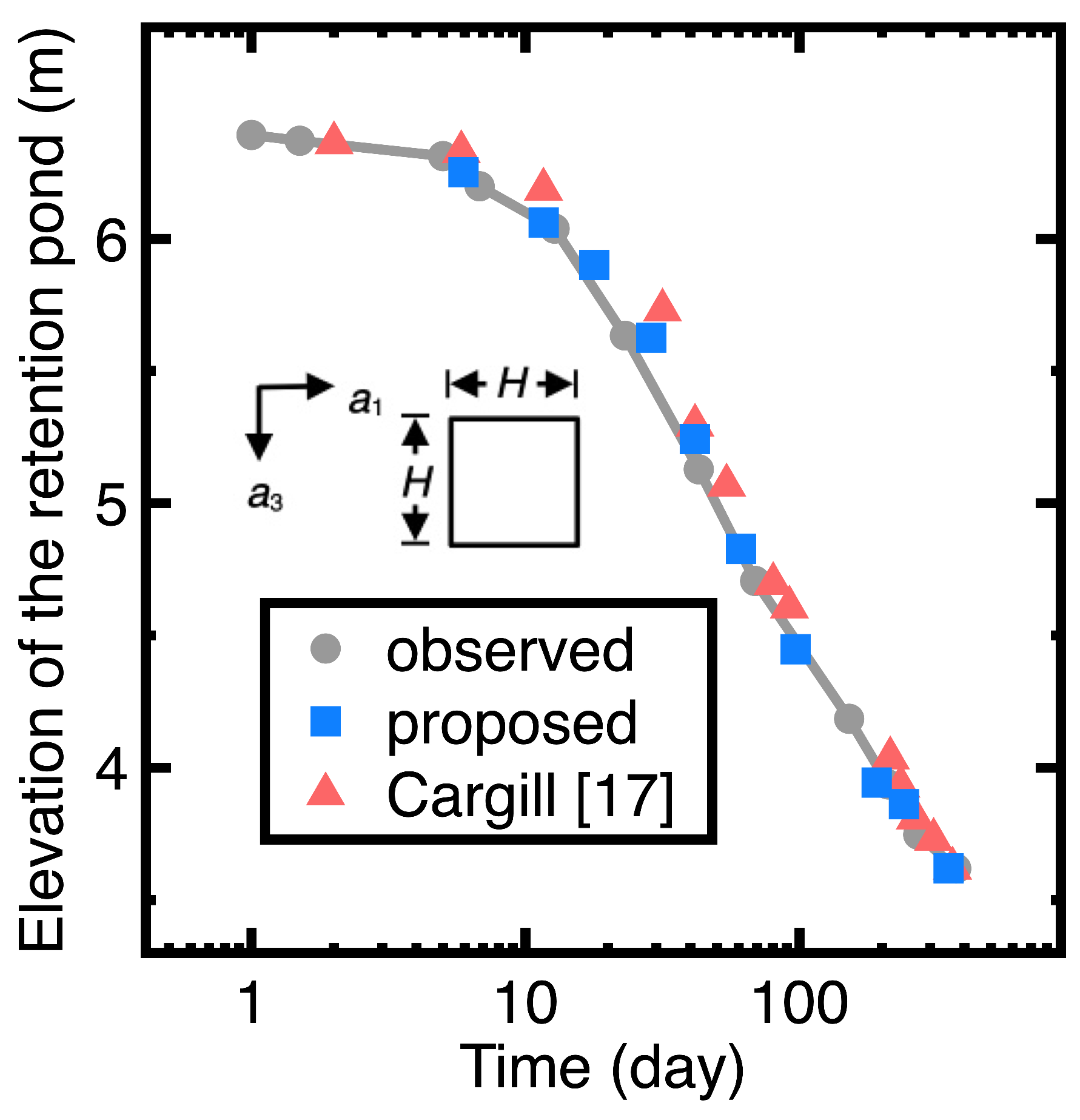
Figure 3.
Predicted , , , and of a phosphate waste layer consolidated by its self-weight at the time t = 30 days
Figure 3.
Predicted , , , and of a phosphate waste layer consolidated by its self-weight at the time t = 30 days
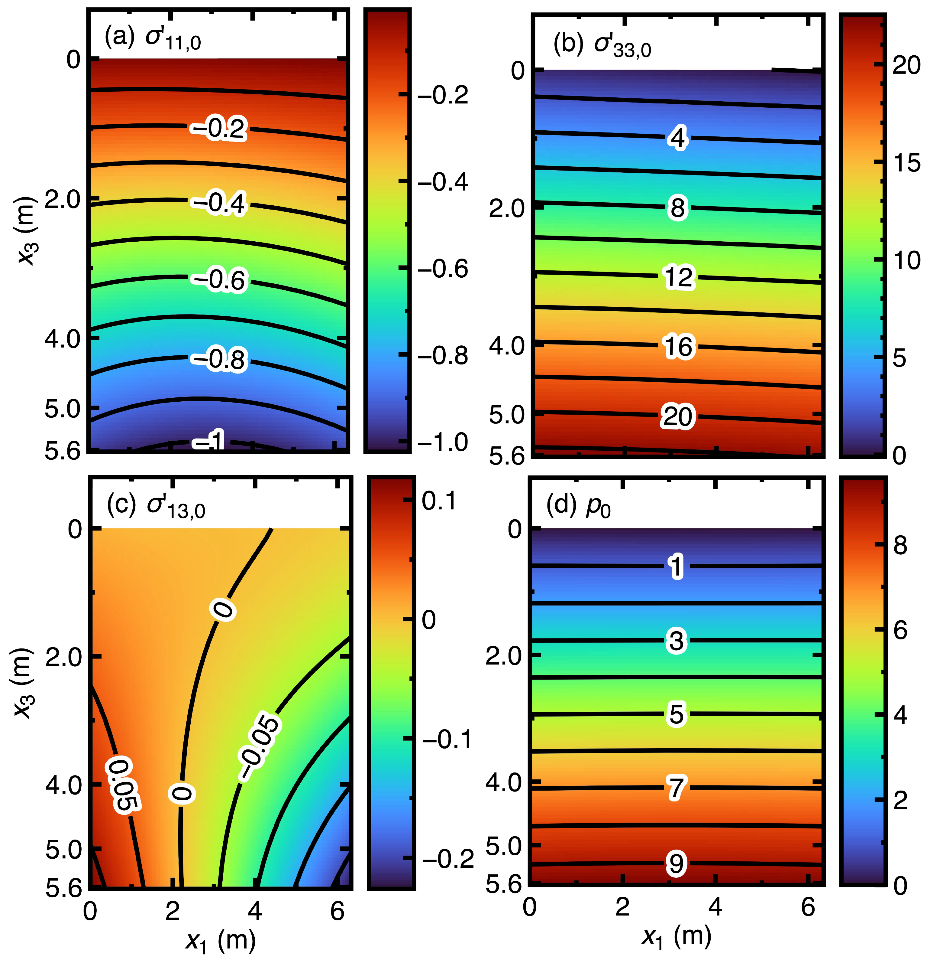
Figure 4.
Convergence of the value in predicting consolidation settlements of a phosphate waste clay layer
Figure 4.
Convergence of the value in predicting consolidation settlements of a phosphate waste clay layer
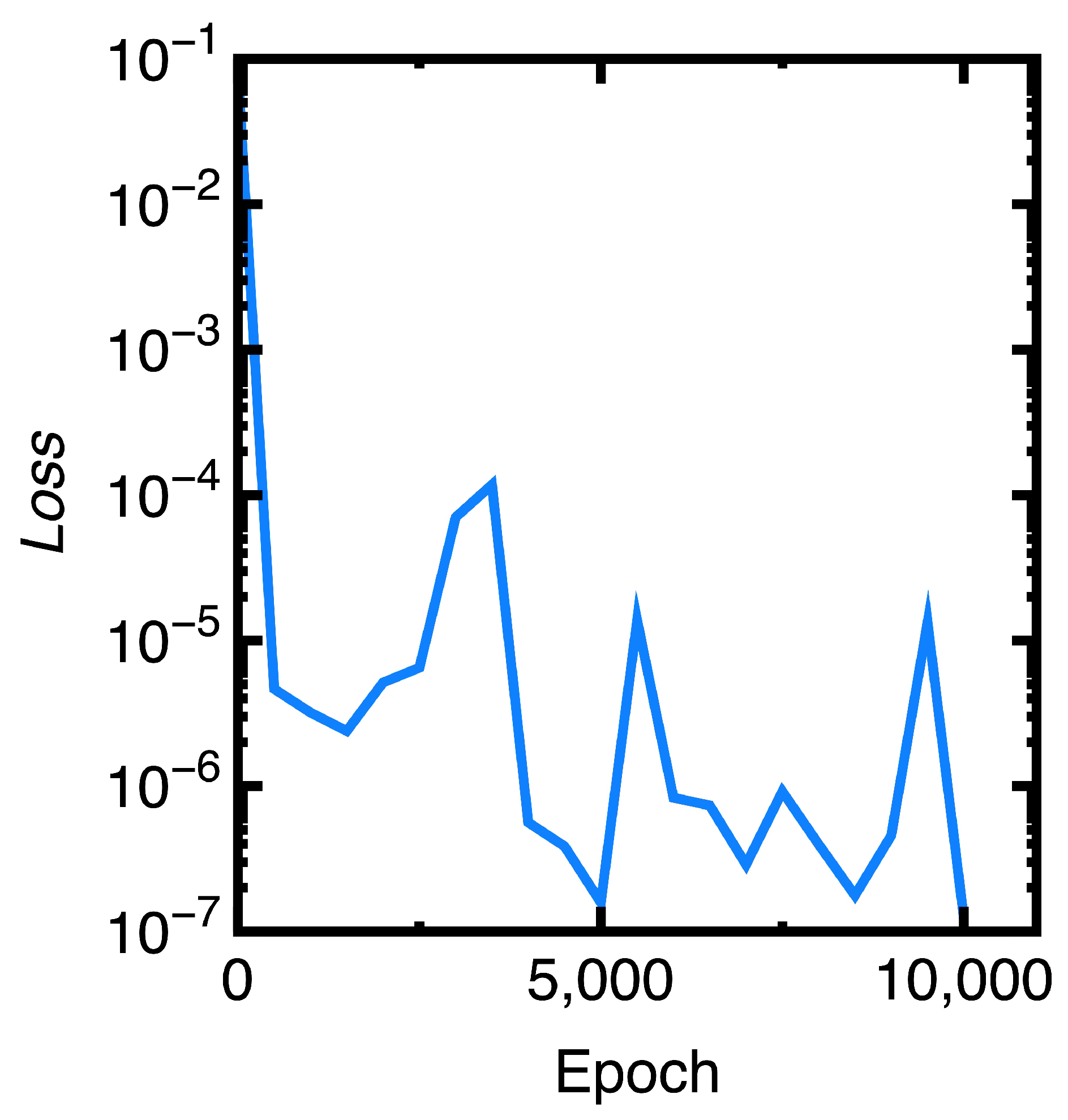
Figure 5.
Comparison of predicted and measured vertical settlements of an Osaka Bay mud layer at the time mins
Figure 5.
Comparison of predicted and measured vertical settlements of an Osaka Bay mud layer at the time mins
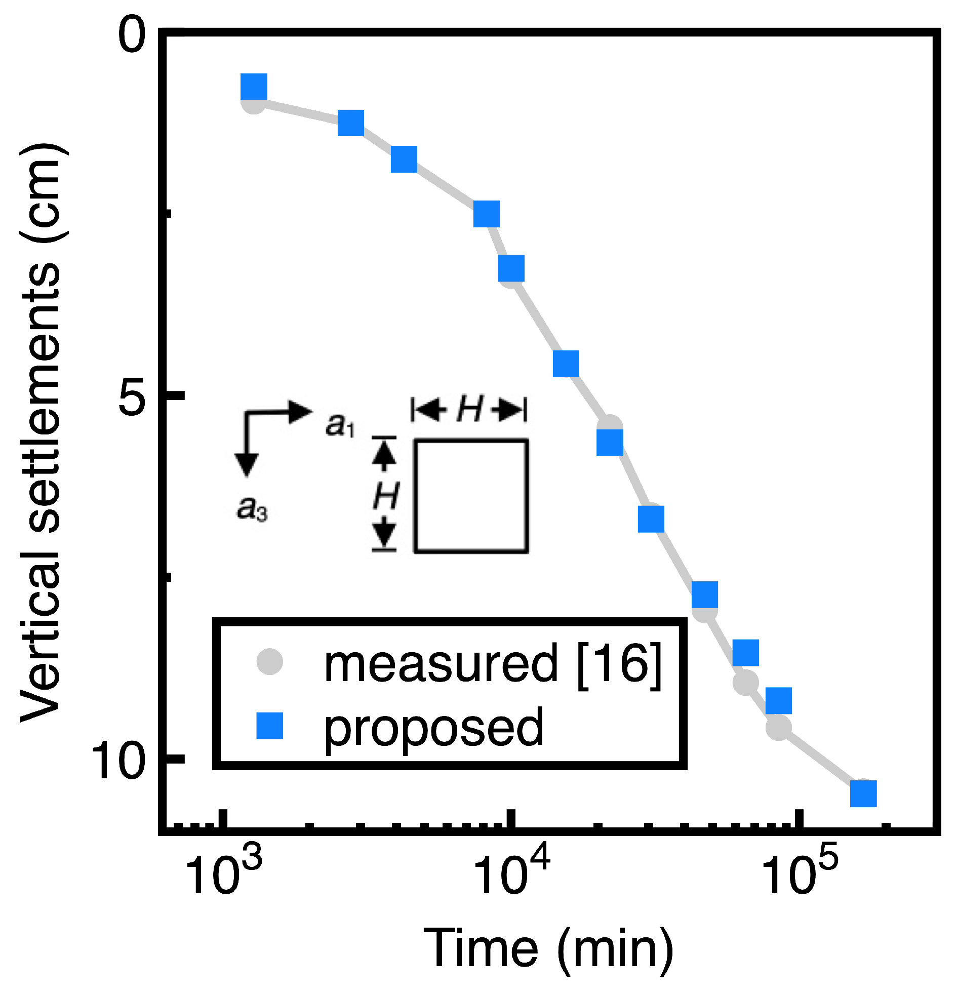
Figure 6.
Predicted , , , and of an Osaka Bay mud layer consolidated by its self-weights at the time mins
Figure 6.
Predicted , , , and of an Osaka Bay mud layer consolidated by its self-weights at the time mins
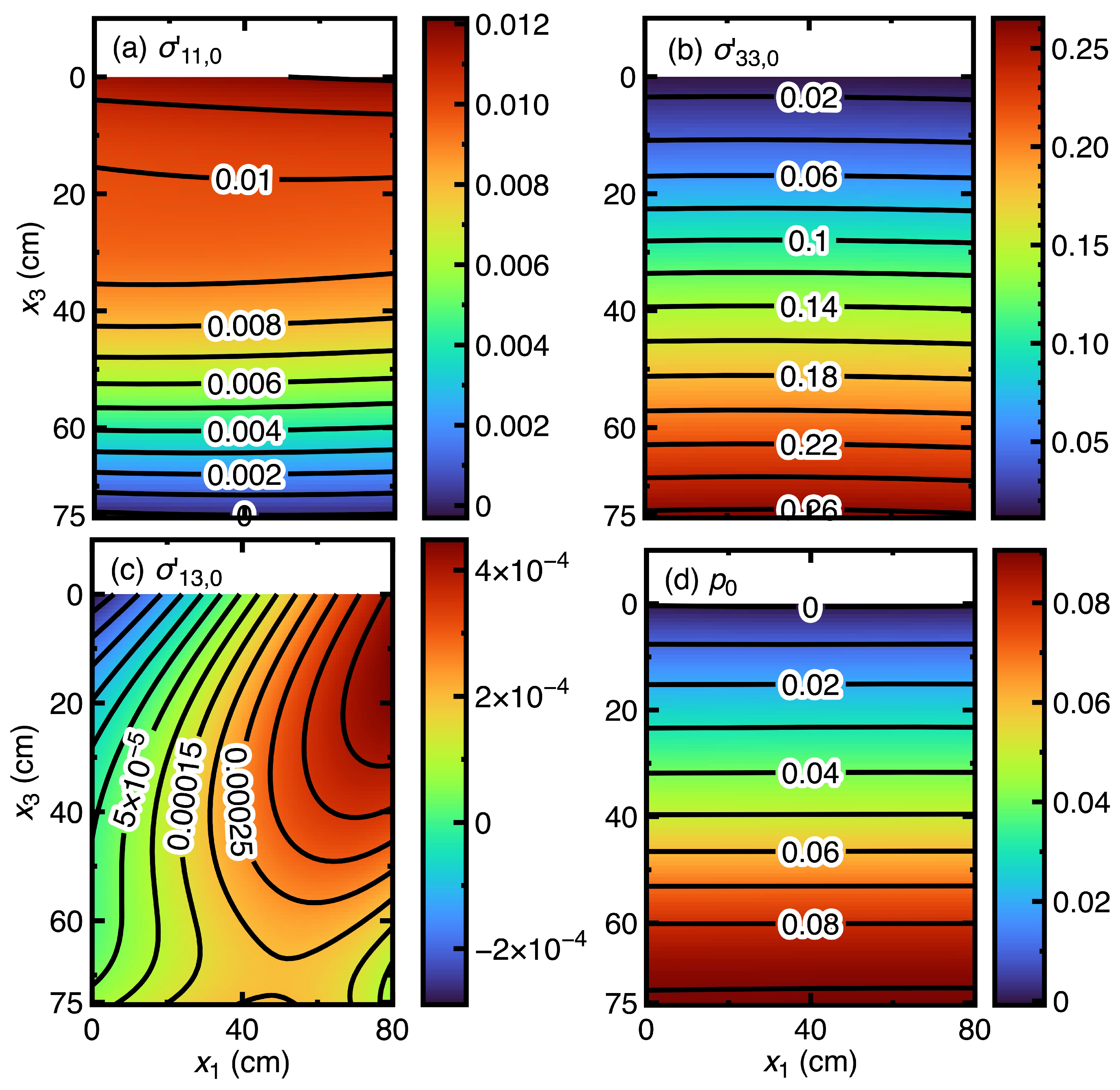
Figure 7.
Convergence of the value in predicting consolidation settlements of an Osaka Bay mud layer
Figure 7.
Convergence of the value in predicting consolidation settlements of an Osaka Bay mud layer
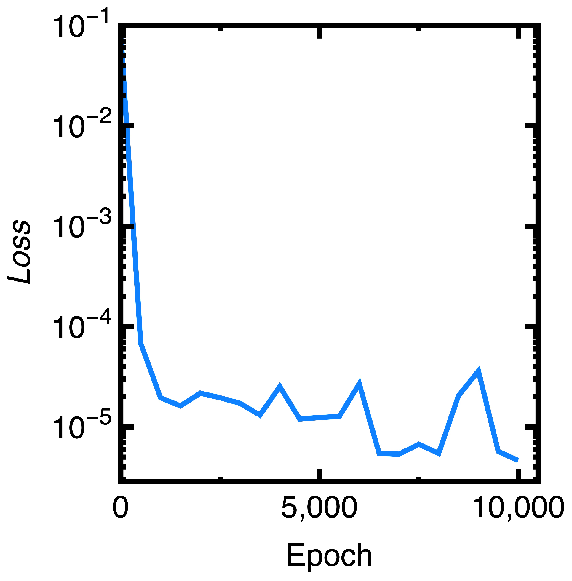
Figure 8.
Comparison of the values with respect to different learning rates : (a) the phosphate waste clay (b) Osaka Bay mud
Figure 8.
Comparison of the values with respect to different learning rates : (a) the phosphate waste clay (b) Osaka Bay mud
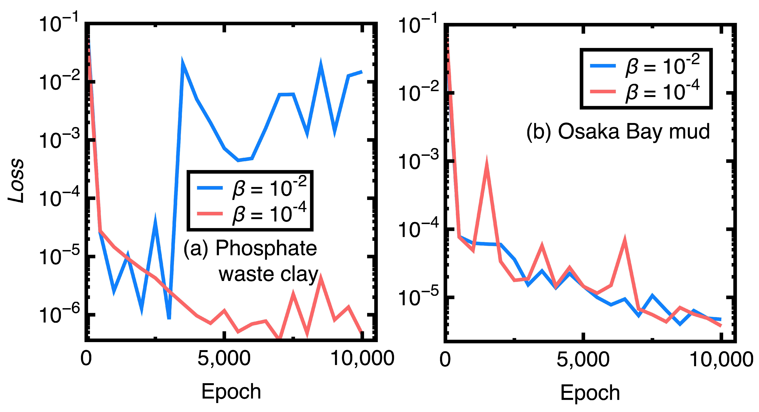
Figure 9.
Comparison of the values with respect to different numbers of interior and boundary nodes: (a) the phosphate waste clay (b) Osaka Bay mud
Figure 9.
Comparison of the values with respect to different numbers of interior and boundary nodes: (a) the phosphate waste clay (b) Osaka Bay mud
Disclaimer/Publisher’s Note: The statements, opinions and data contained in all publications are solely those of the individual author(s) and contributor(s) and not of MDPI and/or the editor(s). MDPI and/or the editor(s) disclaim responsibility for any injury to people or property resulting from any ideas, methods, instructions or products referred to in the content. |
© 2025 by the authors. Licensee MDPI, Basel, Switzerland. This article is an open access article distributed under the terms and conditions of the Creative Commons Attribution (CC BY) license (http://creativecommons.org/licenses/by/4.0/).
Copyright: This open access article is published under a Creative Commons CC BY 4.0 license, which permit the free download, distribution, and reuse, provided that the author and preprint are cited in any reuse.


