
Submitted:
28 August 2025
Posted:
29 August 2025
You are already at the latest version
Abstract
Location-based services (LBS) are well-known services that provide a user’s position and deliver tailored experiences. They are generally used for getting from one location to another, tracking, mapping, and timing, and they are often available in smartphones, tablets, computers, and applications such as Facebook, Twitter, TikTok, and YouTube. Aside from these, the data is collected by location-based services, which can be provided to the data analyst for some business reasons, such as improving marketing strategies, organizational policies, and customer services. In this situation, it can lead to privacy violation concerns. To reduce these concerns when location-based data is provided to the data analyst or released to be utilized outside the scope of data collecting organizations, several privacy preservation models have been proposed, such as k-Anonymity, l-Diversity, t-Closeness, LKC-Privacy, differential privacy, and location-based privacy preservation models. Unfortunately, to the best of our knowledge about these privacy preservation models, they still have several vulnerabilities regarding privacy violation concerns that must be addressed when location-based data is released, i.e., privacy violation issues from inferring sensitive locations (e.g., specialized hospitals, pawnshops, prisons, and safe house), privacy violation issues from considering duplicate trajectory paths (i.e., although the user’s visited path duplicate with other paths, it still has privacy violation issues when it consists of a sensitive location), and privacy violation issues from considering unique locations (e.g., home, condominium, and office). Moreover, these privacy preservation models have data utility issues and data transformation complexity that must be improved. To address these vulnerabilities, a new privacy preservation model, (ξ, ϵ)-Privacy, is proposed in this work. It is based on data generalization and data suppression in conjunction with data sliding windows and R-Tree, such that there are no concerns about privacy violations in its released location-based data from using privacy violation issues from inferring sensitive locations, privacy violation issues from considering duplicate trajectory paths, and privacy violation issues from considering unique locations. It is highly efficient and effective in data maintenance. Furthermore, we show that the proposed model is efficient and effective through extensive experiments.
Keywords:
Privacy Preservation Model
; Sensitive Location
; Location-based services (LBS)
; R-Tree
; Data Sliding Window
; Data Suppression
; Data Generalization
1. Introduction
Global Positioning Systems (GPS) [1,2] are outstanding in location-based applications. They are generally used for getting from one location to another, tracking (i.e., monitoring objects or personal movements), mapping (i.e., creating world maps), and timing (i.e., making it possible to take precise time measurements). They can achieve their objectives by using an appropriately specified GIS technology, e.g., United State’s Global Positioning System (USA’s GPS) [3], Russia’s Global Navigation Satellite System (GLONASS) [4], China’s BeiDou Navigation Satellite System (BDS) [5,6], or so on. Generally, they can be separated into three groups by considering the characteristics of their provided services, i.e., personal GPS, commercial GPS, and military GPS.
The examples of using GPS technologies in personal and commercial real-life applications are maps, trackers, transportation, and delivery services. The well-known map applications are Google Map [7,8], Google Earth [9,10], and OpenStreetMap [11,12]. The well-known tracker applications are portable GPS trackers [13,14,15], Find My on iPhone [16], and Android Find My Device [17]. The well-known GIS transportation is logistic [18,19] and express services [20,21,22]. The well-known delivery service applications are DoorDash [23], Uber Eats [24], Zomato [25], Deliveroo [26], Doordash [27], and FoodPanda [28]. Aside from the applications mentioned above, we found that GPS technologies are proposed to collect data about the user’s visited locations. The data collection of the user’s visited locations is called the trajectory dataset (or sometimes it is called the location-based dataset) [29,30,31,32]. Generally, it is used to show the history of locations that are visited by users. However, we also found that some trajectory datasets allow data analysts to access them for business reasons, such as improving marketing strategies, improving service strategies, analyzing human behaviors, traffic analysis, or providing insights that are valuable for related applications and urban planning. In data analysis situations, in [33,34,35,36,37], and [38], the authors demonstrate that they have concerns about privacy violation issues. An example of privacy violation issues in trajectory datasets is explained in Example 1.
Example 1
(A privacy violation issue in trajectory datasets). We give Table 1 as the specified trajectory dataset that is provided to the data analyst. We assume that the adversary receives Table 1, and the adversary further ensures that a trajectory path (the sequence of the user’s visited locations) in Table 1 is the sequence of Bob’s visited locations. Moreover, we suppose that the adversary strongly knows that Bob visited and , and he/she needs to reveal Bob’s diagnosis from Table 1. In this situation, the adversary can ensure that Bob’s diagnosis is HIV because only can be determined according to the adversary’s background knowledge about Bob.
With Example 1, we can conclude that the unique subsequence of the user’s visited locations in trajectory datasets can have concerns about privacy violation issues. To address these issues, LKC-Privacy [33] and its extended models [39,40,41,42,43] are proposed. They have the assumption of privacy preservation in trajectory datasets that the adversary only has the background knowledge about the subsequence of the target user’s visited locations to be at most L locations, and they are based on data suppression [44]. That is, the trajectory datasets do not have any concerns of privacy violation issues when all unique L-size subsequences of the user’s visited locations are suppressed to be at least K indistinguishable paths. Furthermore, every sensitive value relates to each indistinguishable L-size subsequence of the user’s visited locations; it must have the confidence of data re-identification to be at most C. An example of privacy preservation in trajectory datasets with LKC-Privacy is explained in Example 2.
Example 2
(Privacy preservation with LKC-Privacy). We suppose that Table 1 is the specified trajectory dataset that is provided to the data analyst. For privacy preservation, let the value of L and K be 2. Let the value of C be 0.70. For privacy preservation with these given privacy constraints, all unique 2-size subsequences of the user’s visited locations in Table 1 are suppressed to be at least 2 indistinguishable subsequences. Furthermore, all diagnoses were normalized to the confidence of data re-identification to be at most 0.70. Therefore, a data version of Table 1 does not have any concerns about privacy violation issues; it is shown in Table 2. With Table 2, we can see that the confidence of data re-identification for every diagnosis from considering each 2-size subsequence of the user’s visited locations is at most 0.70 (or 70%).
In addition, we can see that Table 2 is more secure in terms of privacy preservation than its original (Table 1). However, it loses some meaning of data utilization. Generally, data utility and data privacy are a trade-off. However, we found that KLC-Privacy has serious vulnerabilities that must be considered when it is used to address privacy violation issues in trajectory datasets. The vulnerabilities of LKC-Privacy will be explained in Section 2.
The organization of this work is as follows. The motivation of this work is presented in Section 2. Then, the model and notation of this work will be presented in Section 3. Subsequently, the experimental results will be discussed in Section 4. Finally, the conclusion and future work of this work are discussed in Section 5 and Section 6, respectively.
2. Motivation
Privacy violation is a serious issue when the data holder allows the data analyst to access datasets. To address this issues, there are several privacy preservation models to be proposed such as k-Anonymity [45], l-Diversity [46], t-Closeness [47], and their extended models that are presented in [48,49,50,51,52,53,54]. The privacy preservation idea of these models is as follows.
- The attributes of datasets are separated into explicit identifier attributes, quasi-identifier attributes, and sensitive attribute(s).
- All values in every explicit identifier attribute must be removed.
- The re-identifiable quasi-identifier values are suppressed or generalized by their less specific values to be indistinguishable.
- In addition, some privacy preservation models (e.g., l-Diversity and t-Closeness) further consider the characteristics of sensitive values in their privacy preservation constraints.
Although these preservation models can be used to address privacy violation issues when datasets are released, they still have several issues that must be addressed, e.g., data utility issues and the high complexity in terms of data transformations. To address the vulnerabilities of these models, the differential privacy model [55] is proposed. This privacy preservation model is based on a data query framework in conjunction with the noise of data and data re-identification probability. That is, the data holder does not allow the expert to utilize the dataset directly. The dataset can be utilized by the expert via the data query framework such that the query result is accorded by the given data re-identification probability. If an arbitrary query result does not accord with the given data re-identification probability, they are returned with the appropriate noise. Unfortunately, the mentioned above privacy preservation models mentioned above are often insufficient to address privacy violation issues in trajectory datasets (or location-based datasets). That is because they are proposed to address privacy violation issues in datasets that have each quasi-identifier attribute as a different data domain, e.g., . While the quasi-identifier of trajectory datasets is the sequence of user’s visited locations, e.g., . To rid this vulnerability in these models, the privacy preservation models for trajectory datasets are proposed [33,34,35,36,37,38]. One of the well-known privacy preservation models for trajectory datasets is LKC-Privacy [33]. This privacy preservation model uses three privacy parameters (i.e., L, K, and C) to limit privacy violation issues when the data holder allows the data analyst to access trajectory datasets. An example of privacy preservation in trajectory datasets with LKC-Privacy is explained in Example 2. Although LKC-Privacy can be used to address privacy violation issues in trajectory datasets, we found that it still has serious vulnerabilities that must be addressed, i.e., data utility issues, complexities, and data streaming issues. Moreover, LKC-Privacy is only appropriate to address privacy violation issues in the static trajectory dataset, which has attributes strongly separated into the sequence of the user’s visited locations and their related sensitive values. In addition, the sensitive locations (e.g., specialized hospitals, pawnshops, prisons, and safe houses) are not considered in the privacy preservation constraint of LKC-Privacy. For this reason, although trajectory datasets are satisfied by LKC-Privacy constraints, they still raise concerns about privacy violation issues from inferring sensitive locations that must be addressed. An example of privacy violation issues from inferring sensitive locations is shown in Example 3.
Example 3
(Privacy violation issues from inferring sensitive locations). We suppose that Figure 1 is the specified location-based graph that is proposed to represent five sequences of the users’ visited locations. Moreover, we assume that the location is a serious or sensitive location, i.e., we suppose that it represents a cancer hospital (i.e., it is a specialized hospital). Therefore, if the adversary can indicate that users who visited the location , the adversary can infer that they have symptoms of cancer.
Moreover, we found that LKC-Privacy [33] and the trajectory privacy preservation models that are presented in [34,35,36,37,38,39,40,41,42] and [43], also have a vulnerability about privacy violation issues when considering duplicate trajectory paths. It is demonstrated in Example 4.
Example 4
(Privacy violation issues from considering duplicate trajectory paths). We assume that John is the target user of the adversary. Moreover, we assume that the adversary ensures that a sequence of locations in Figure 1 is the sequence of John’s visited locations. The adversary further knows that John visited both locations and . In these situations, the adversary can see that there are both subsequences of locations (i.e., and ) that are according to the adversary’s background knowledge about John. However, the adversary still ensures that a user visited the location to be John. Therefore, we can conclude that the number of satisfied subsequence occurrences of the visited locations of the users does not have any effect on the confidence of the adversary in inferring the users who visited the location .
Another vulnerability of these privacy preservation models is that they do not consider the type of locations, such as the identifier locations, the relationship locations, and the sensitive. In addition, the relationship locations represent the locations between the next location of the initially specified locations and the location that is before the specific ending location. The sensitive locations are where the user does not need other people to know when he/she visited them because they can lead to privacy violations, such as prisons, specialized hospitals, pawnshops, or safe houses. The starting locations are often a (unique) private location of users such as users’ homes, condominiums, or offices. They can be used to be the explicit identifier value for re-identifying the data owner. An example of privacy violation issues from considering unique locations is demonstrated in Example 5.
Example 5
(Privacy violation issues from considering unique locations). We suppose that the adversary knows that Bob’s family lives at the location . Moreover, we assume that the location is a pawnshop, and the location is an elementary school. We assume that Bob lives with his daughter is 5 years old. In this situation, the adversary can ensure that one of Bob’s family members goes to the pawnshop, and another person goes to the elementary school. Therefore, the adversary can infer that Bob’s family has a financial problem, and he/she can assure that Bob goes to the pawnshop because Bob’s daughter is prohibited by law (she is a child).
With Examples 3, 4, and 5, we can conclude that LKC-Privacy [33] and the trajectory privacy preservation models that are presented in [34,35,36,37,38,39,40,41,43,56], they still have the vulnerabilities about privacy violation issues that must be addressed. To address these vulnerabilities of these privacy preservation models, a new privacy preservation model is proposed in this work; it will be presented in Section 3.
3. Model and Notation
3.1. The Graph of Users’ Visited Sequence Locations
In this section, we present the characteristics of graphs that are proposed to represent the users’ visited sequence locations. Let be the set of users. Let be the set of all possible timestamps that the users visited each location. Let be the set of all possible locations. Let = be the sequence of locations that are visited by the user , i.e., the user visited the locations from the timestamp , respectively. Let be a directed graph that is proposed to represent the sequence of locations that are visited by every user . That is, is the set of vertices such that each vertex represents an element of that does not include user identifier data, i.e., every element of in is presented in the from of . be the set of edges. With every vertex that only has the indegree(s), it must be according to the property as such that is the timestamp of each connected indegree vertex of . While each vertex only has the outdegree(s), it must satisfy the property as such that is the each connected outdegree vertex of . Every vertex has both in and out degrees; it must satisfy the properties as follows.
- Let the vertex connects to the vertex .
- Moreover, let the vertex connects to the vertex .
- Therefore, the timestamp of the vertices , . must be according to the property as .
We found that each vertex of generally has a different ability to re-identify the data owner. For this reason, we can divide each vertex into an appropriate level by considering its ability for data re-identification when it is provided to the data analyst. Typically, the first vertex (the starting point) of each path in has the ability of data re-identification to be more than other vertices in the path because it usually represents a private location of users, e.g., a house or a condominium. Moreover, we can see that the endpoint of each path in often has the ability of data re-identification to be less than other vertices.
Definition 1
(The level of data re-identification). Let be a non-indegree-vertex. Let be a non-outdegree-vertex. Let be a sequence of vertices in from to . Let , , …, be the distance between and , between and , …, and between and , respectively. The level of → can be denoted as , , …, , respectively.
For example, let be the set of all possible users. Let be the set of all possible locations that can be visited by the users. Let be the set of the possible timestamps. We suppose that the sequence of locations was visited by to be , , , , and in the timestamp that is , , , , and , respectively, i.e., →→→→. The sequence of locations was visited by to be , , , and such that he/she visited these locations in the timestamp that is , , , and , respectively, i.e., →→→. The user visted the locations , , , , and in the timestamp that is , , , , and , respectively, i.e., →→→→. The locations , , , and in the order of the timestamp as , , , and and the locations , , and in the order of the timestamp as , , and are the sequence of the and ’s visited locations, respectively, i.e., →→→ and →→. With these given instances, the graph of users’ visited sequence locations is shown in Figure 2. With this graph, we can see that the vertices , , , and do not have any indegree. Thus, they are available at level 0. Moreover, we found that the vertices , , and have a distance from their related vertex in level 0 that is less than other vertices. Thus, they are available at level 1. With the vertices that have the distance between them and their related vertex at level 0 being 2, they are the vertices , , and . Thus, these vertices are available at level 2. Only the vertex has the distance between it and its related vertices in the level 0 to be 3, so only this vertex can be available in the level 3. In addition, the unconsidered vertices (i,e., and ) are available in the level 4.
3.2. The Type of Vertices
In this section, we describe the characteristics of vertices in that are considered in the proposed privacy preservation constraint, i.e., the sensitive vertex and the unique vertex. The sensitive vertex is an arbitrary vertex that represents the sensitive location (e.g., specialized hospitals, pawnshops, safe houses, or prisons) that is visited by the user(s). They can raise concerns about privacy violation issues when they are utilized outside the scope of the data-collecting organization. Thus, the data holder must ensure that when is provided to the data analyst, every sensitive vertex must be protected by an appropriate privacy preservation technique. An example of privacy violation issues in from considering the sensitive vertex is explained in Example 6.
Example 6
(Privacy violation issues from considering sensitive vertices). We assume Jenifer has a diagnosis of cancer. The history of Jenifer’s visited locations is a sequence of users’ visited locations in . We further assume that Jennifer is a target user of the adversary, such that the adversary needs to disclose Jenifer’s disease from . Moreover, the adversary knows that a location in the sequence of Jenifer’s visited locations is a specialized hospital for treating cancer. In this situation, the adversary can infer that Jennifer has a health problem with cancer.
Another type of vertices is also considered in the proposed privacy preservation constraints, it is the unique vertex, i.e., an arbitrary vertex of represents the user’s house, office, or other unique locations. With this vertex, the adversary can use to identify the sequence of the target user’s visited locations in . An example of privacy violation issues in from considering the unique vertex is explained in Example 7.
Example 7
(Privacy violation issues from considering unique vertices). Let Emma be the target user of the adversary. Let Figure 2 be the that is provided to the data analyst. We assume that the adversary strongly believes that the provided contains the sequence of Emma’s visited locations. Let the location be a pawnshop (a private or sensitive location). Moreover, we assume that the adversary knows that the location of Emma’s house is . In this situation, the adversary can ensure that Emma goes to a pawnshop. Therefore, the adversary can infer that Emma has a financial problem.
With Examples 6 and 7, we can conclude that the sensitive vertex and the unique vertex can lead to privacy violation issues when is provided to a data analyst.
3.3. Data Sliding Windows [56,57,58,59]
Generally, the location graph is very large or extensive. Furthermore, it is very complex. Thus, it often uses more execution time in data processing. However, to the best of our knowledge about the data processing of the location graph , we found that it is often processed (or utilized) in the form of the newest data to the oldest data or according to the specified period of times. For this reason, we can use data sliding windows to increase the efficiency of data processing in the location graph . The idea of increasing the efficiency of data processing by using the data sliding window is that the size of the location graph is separated to be small.
Definition 2
(Data sliding windows). Let be the specified location graph. Let and be the specified period times such that is the initial time and is the end time, where <. Let be the data sliding window function that is proposed for sliding to become . That is, are the subgraphs of , i.e., ⊆, so that they only collect the vertices and edges of that are available in the timestamp between and .
An example of utilizing in the form of the newest data to the oldest is that the data holder creates a dynamic report by considering the sequence of users’ visited locations from the last ten months to make the appropriate traveling paths for tourists. In addition, an example case of generating reports from by specifying the period of times is that we suppose that the data holder needs to build a report to show the frequency of users who visited each location between September 2024 and December 2024.
3.4. Location Hierarchy
3.4.1. Dynamic Location Hierarchy
R-Trees are tree data structures that are proposed to present and index multidimensional information [60,61] such as geographical coordinates, rectangles, and polygons. They have been proposed since 1984 by Antonin Guttman [62]. They are often available in real-world map applications to store spatial objects such as restaurant locations and the polygons that typical maps are made of streets, buildings, outlines of lakes, and coastlines, and then find answers to the specified question, e.g., find all universities within one kilometer of the current visited location, retrieve all road segments in the range of one kilometer from considering the visited location, or find the nearest hospital. R-Trees can further accelerate nearest-neighbor search for various distance metrics, including great-circle distance. That is, all the objects of interest lie within this bounding rectangle. A question that does not intersect the bounding rectangle cannot intersect any of the contained objects.
Definition 3
(Non-overlapped R-Tree). Let be all possible rectangles that form the boundary of in . Every , where , includes both of information as and the set of the specified locations such that is the label of . Let R-Tree be a tree data structure such that it is constructed from R by the conditions as follows.
- The bounding rectangle is not covered by others, it is the root of R.
- The child of is every that is only covered by and is not covered by others.
- The label of each vertex in the tree is represented by .
An example of R-Trees that are constructed from the location graph . Let each blue cycle in Figure 3(a) represent a location that was visited by the user(s). Let all rectangles (i.e., red, blue, brown, purple, and black rectangles) be the bounding of the specified locations such that the red rectangle is the largest and the black rectangle is the smallest. With these location bounds, an R-Tree version of them is shown in Figure 3(b).
3.4.2. Manual Location Hierarchy
The manual location hierarchy is another way that can also be used to construct the R-Tree of the location graph . It can be built by the location data expert, e.g., the R-Tree of locations can be presented by urban zoning, roads, or other data utilization reasons. All locations are available in the lower level; they must be more specific than all locations that are available in the higher level. Or we can say that each most specific location is presented by a vertex that is available in level 0 (the leaf vertex), and the lowest specific location is presented by the root of the hierarchy.
Definition 4
(Manual Location Hierarchy). Let be a manual location function for the locations from level l to level such that all locations in level l are more specific than level . Moreover, the locations of every level do not overlap, i.e., , and . With the manual location hierarchy function, the location hierarchy of can be presented as a location sequence from level 0 to level l, . In addition, after that, we call the location hierarchy of from level 0 to level l to be .
3.5. Data Suppression
In this section, we propose a data suppression technique that can be used to eliminate the ability of data re-identification in . As we know, the level of identifiable data for the vertices in can be defined by the order of the vertices available in . An example of leveling the vertices of is shown in Figure 2, i.e., the level of each vertex can be defined from the first visited location (the starting point) to the last visited location (the endpoint). That is because the first visited location of each sequence of the user’s visited locations generally can identify that it is higher than others, and we further found that the last visited location of each sequence of the user’s visited locations often has the lowest identifiability. The highly identifiable data of the first visited location is due to its being generally unique and private; it is often the location of the user’s house or office. For this reason, we can define the identifiable data level for every sequence of the user ’s visited locations in from to by the order of them, i.e., , where is the location as the starting point and is the location as the endpoint. With this property of the user’s visited locations is , we can use it to address privacy violation issues (or decrease the ability of data re-identification) in . That is, before is provided to the data analyst, the users’ data privacy in is maintained by suppressing the unique vertices, -Suppression.
Definition 5
(-Suppression). Let be the specified graph of the users’ visited sequence locations such that its vertices are separated into l levels. Let represent the vertices that are available in the levels , …, and , respectively. Let ξ be a positive integer, and it is the suppression constraint of . Let , where , be each specified subgraph of . Let be the function for suppressing the unique vertices of to become . That is, are a forest graph version of such that are satisfied by the the properties that are as follows.
- .
- ∪…∩∪…∪=∅ such that is the set of the vertices in level l of , where .
- ∪…∪∪…∪=.
3.6. Data Generalization
Aside from the identifiable data level of vertices, the proposed privacy preservation model is further based on another major assumption about privacy violation issues: the privacy data of the target user in can be violated by considering a sensitive vertex (a sensitive location), although there are more than one user who visited this vertex. An example of privacy violation issues from considering the specified sensitive vertex and the duplicate paths is illustrated in Examples 3 and 4, respectively. To address these privacy violation issues, before is released, the sensitive vertices are generalized by their less specified values to be indistinguishable. In addition, the less specified values of the sensitive vertices in are presented by a Non-overlapped R-Tree that is satisfied by Definition 3 or a Split-Halves R-Tree that is satisfied by Definition 6.
Definition 6
(Split-Halves R-Tree). Let W be the width of the area where the locations are available in . Let H be the height of the area where the locations are available in . Let be all possible bounding rectangles that can be constructed from . That is, is firstly the bounding rectangle that is constructed, it has the size to be , i.e., it covers all locations of . After that, is divided half to be and , where , , and , until only one remains in a rectangle such that it is separated by considering the width first then the height is considered. Finally, all bounding rectangles are presented in the form of a tree data structure, which is denoted as , such that each bounding rectangle is a vertex and the label of each vertex is presented by the label of the bounding rectangle. That is, is the root of . The child of every is constructed from each that is covered by , but others do not cover it. Each leaf vertex of is represented by a bounding rectangle that covers a location. Let be the possible level of . The levels of are arranged according to the data specification. That is, the root of is available in the level . All leaf vertices are available in the level .
An example of creating the bounding rectangles of with Definition 6 is shown in Figure 5. With Figure 5(a), the first bounding rectangle is created such that it covers all locations that are available in . With Figure 5(b), (c), and (d), the location areas are divided by considering the width first then the height is considered such that are the label (the name of the specified area) of the bounding rectangle 1 to 15, respectively.
Definition 7
(-Generalization). Let ϵ be a positive integer; it is the generalization constraint such that it is in the range between 0 and l. Let or be the data structure that presents the generalized values for each specified vertex v in . Let be the specified vertex. The generalized data version of is the visited time and the . With , the of is the bounding rectangle of in the level ϵ of . With , the of is the label of in the level ϵ of .
3.7. The Proposed Privacy Preservation Model
3.7.1. Problem Statement
Let be a directed graph that represents the sequence of users’ visited locations. Let be the set of sensitive locations that are available in . Let be the data generalization constraint. Let or be the data structure that is proposed to present the level of locations in such that it is the reference of the specific location levels that can be used to generalize the unique locations in to be indistinguishable. Let be the data suppression constraint for suppressing the unique locations in to be indistinguishable, i.e., it is another data distortion technique that is also used to distort the unique locations in to be indistinguishable. Let and be the period time of the specified locations in such that is the initial time and is the end time, where <. Let be a privacy preservation function, i.e., it is proposed for transforming to become . That is, the vertices of are slided by and to be . All unique locations of are suppressed by . Moreover, each sensitive location is generalized by its less specific values that are available in the level of or .
3.7.2. The Privacy Preservation Algorithm
In this section, we devote to presenting an algorithm that can be used for transforming to satisfy the proposed privacy preservation constraints, which is shown in Algorithm 1. With this algorithm, it has seven inputs, i.e., , , , , , , and . That is, is the specified graph that represents the sequence of users’ visited locations. is the sensitive vertices, the sensitive locations, that are available in . is or that is proposed to represent the data specification level of each sensitive vertex in . and are the period time of the specified vertices in such that is the initial time and is the end time, where <. is the data suppression constraint for suppressing the unique vertices in . Another input of the proposed algorithm is , which is the data generalization constraint for generalizing each sensitive in . The output of this algorithm is that are satisfied by , , , and .
|
Algorithm 1:
, , , , , , )-Privacy
|
|
To achieve the proposed privacy preservation constraints in , the algorithm first slides (or spits) the vertices of to be by . That is, the vertices of do not occur in the timestamp between and , they are not ignored because they are available in the outside scope of the data collection for publishing uses. Then, the unique vertices are available in the levels 0, …, , and of to be suppressed. Thus, the output of this step is a forest of , i.e., . Subsequently, are iterated. Furthermore, every sequence of vertices in , where , is also iterated. The vertices of are further iterated. If the algorithm found the sensitive vertex , it is generalized by its less specific value that is available in the level of . Finally, the algorithm returns that are satisfied by and .
In addition, with the complexity of the proposed privacy preservation algorithm, if we only consider the data distortion that is based on data suppression, we can see that only the number of paths and the level of the suppressed vertices can affect the data suppression processes. Therefore, the complexity of data suppression processes of the proposed privacy preservation algorithm can be defined by Equation 1.
where,
- is the level of vertices that are suppressed.
- n is the number of the paths of .
With the data generalization, we can see that its complexity is based on the number of forest graphs of , the number of sensitive locations, the number of vertices in each forest graph, and the height of . Therefore, the complexity of data generalization for each forest graph can be defined by Equation 2. For this reason, the data generalization complexity of the proposed privacy preservation algorithm can be defined by Equation 3.
where,
- n is the number of users’ visited location in .
- is the number of sensitive locations that must be protected in .
- is the number of the paths that are available in of .
- l is the high of .
where,
- are the forest graphs of .
Therefore, the complexity of the proposed privacy preservation algorithm can be defined from its data suppression and data generalization processes, i.e., it can be defined by Equation 4.
3.7.3. Utility Measurement
With the proposed privacy preservation algorithm that is presented in Section 3.7.2, we can see that can achieve privacy preservation constraints by suppressing and generalizing the unique vertices and the sensitive vertices to be indistinguishable. For this reason, a metric is necessary to measure the utility of the data.
With data suppression, the unique vertices in are removed until they satisfy the proposed privacy preservation constraint. Generally, each removed vertex directly affect the data utility of . Therefore, the data utility or the penalty cost (or the data loss) of can be defined by Equation 5. More penalty cost of Equation 5 leads to the low data utility in .
where,
- is the number of paths in .
- is the number of vertices in .
- is the number of suppressed vertices in .
With data generalization, sensitive vertices are distorted by their less specific values to satisfy the proposed privacy preservation constraint. In addition, generalized vertices affect the data utility of . Thus, a data utility metric is necessary to measure the data utility of the generalized is necessary; it is shown in Equation 6. The higher penalty cost of Equation 6 leads to the low utility of the data in .
where,
- represents the level of generalization of the data of the vertex .
- is the highest of .
Therefore, the utility of the data or the penalty cost of can further be defined by Equation 7. The low penalty cost of Equation 7 for is desired.
In addition to Equation 7, the utility of the data of can be measured using a relative error metric [63]. With this metric, the utility of the data or the penalty cost of is based on the difference between the original query result and the result of the related experiment query. The higher cost of the relative errors means that has low data utility. The relative error of can be defined by Equation 8.
where,
- v is the original query result.
- is the result of the related experiment query.
4. Experiment
In this section, we present the experiments conducted to evaluate the proposed algorithm in terms of both effectiveness and efficiency. The effectiveness is assessed using two measures, utility loss and relative error. Utility loss, measured by the , evaluates the quality of data after the anonymization process. The relative error was evaluated between the original query results and the experimental query results with different query types, including full scan, partial scan, and range scan. Efficiency is evaluated based on the total execution time required for the anonymization process.
4.1. Experimental Setup
We evaluated our proposed framework using two well-established trajectory datasets, City80k and Metro100k, which have been widely adopted in trajectory data privacy research [64,65,66].
The City80k dataset simulates the movement trajectories of 80,000 citizens navigating through a metropolitan area. It records movements across 26 city blocks over a 24-hour period, reflecting realistic urban mobility patterns. Each trajectory is represented as a sequence of visited locations in the format location_id, where locations are denoted by alphanumeric codes such as , , and . The dataset also contains five disease categories as sensitive attributes, namely HIV, Cancer, SARS, Flu, and Diabetes. These sensitive attributes were not utilized in this research.
The Metro100k dataset is designed to represent the transit patterns of 100,000 passengers traveling within the Montreal subway system. Passenger movements are recorded across 65 stations within a 60-minute time window, resulting in 3,900 possible spatio-temporal combinations derived from 65 locations and 60 time units. Each point in a trajectory is presented in the form of indicates location 28 at timestamp . Five employment status categories are included as sensitive attributes, namely On-welfare, Full-time, Retired, Part-time, and Self-employed, but these sensitive attributes were not used in this investigation.
Our experiments were carried out on an Intel Core i7-6700 3.40GHz PC with 16GB RAM while following the experimental setup described in related trajectory privacy research. The experimental evaluation focused on the trade-off between privacy protection and data utility preservation under different parameter configurations, including the number of suppressed timestamps (), the number of generalized locations (), the level of Manual Location Hierarchy (), and the dataset size.
4.1.1. Effectiveness
In the first part of the experiment, we examine the effectiveness of the algorithms by varying the numbers of , , and the level of . Effectiveness is evaluated using utility loss and results are presented on a logarithmic scale. To enhance robustness, each data point in the plots represents the average value obtained from three independent random trials.
In Figure 6(a) and (b), we examine how increasing privacy-preserving parameters affects utility loss. In Figure 6(a), we vary the number of from 1 to 5 timestamps while keeping the number of at 1, the level of at 1, and using the complete dataset. In Figure 6(b), we vary the number of from 1 to 5 locations while fixing the number of at 0, the level of at 1, and using the complete dataset (100%).
Both experiments demonstrate a consistent pattern where utility loss increases as privacy-preserving parameters increase. This occurs because uniform frequency distributions across different locations, where each location exhibits similar occurrence counts, and suppressing multiple timestamps from the dataset leads to increased data distortion and reduced dataset utility for analysis. These findings confirm the expected trade-off between privacy protection and data utility.
In Figure 6(c), we analyze the effect of on utility loss in the context of at 0, at 1, and using the complete dataset (100%). In this experiment, is varied from level 1 to the maximum level 4. The represents the Manual Location Hierarchy, which is another way to construct the R-Tree of the location graph and is typically designed by location data experts. It can be organized according to criteria such as urban zoning, road networks, or other application-specific considerations, and is structured into multiple levels, where the lower levels represent more specific locations and the higher levels represent more general locations, with Level 0 corresponding to the raw data. More general locations improve privacy preservation but reduce spatial granularity.
The results indicate that the utility loss increases when the level of increases for both datasets (City80k and Metro100k). This is expected because generalizing locations to higher levels in the hierarchy reduces the resolution of the data, making it less useful for fine-grained analysis. Moreover, the City80k dataset shows consistently higher utility loss compared to Metro100k, probably due to its more diverse distribution of individual movements.
In Figure 6(d) and (e), we investigate how the size of the dataset affects utility loss under different privacy configurations. In Figure 6(d), we vary the dataset size from 20% to the complete dataset while keeping the number of at 0, the number of at 1, and at 1. In Figure 6(e), we conduct a similar experiment but with increased to 1, while maintaining the number of at 1 and the at 1. The comparison shows that when increases from 0 to 1 in Figure 6(e), a higher value of utility loss is observed compared with Figure 6(d), due to the suppression of one timestamp. However, both experiments show relatively stable utility loss as the dataset size increases. This stability can be explained by the stratified sampling approach that preserves the proportional structure of the dataset. Despite applying privacy-preserving techniques such as timestamp suppression or location generalization, the uniform frequency distributions across different locations are preserved across all sizes of the dataset.
4.1.2. Efficiency
After the characteristics of the proposed algorithm in terms of effectiveness have been demonstrated, subsequently, the efficiency of the algorithm, i.e., the execution time, is considered. We investigated efficiency with regard to the numbers of , , the level of , and dataset size. To ensure robustness, each plotted data point represents the mean value computed from three independent random trials.
In Figure 7(a), we vary the number of from 1 to 5 timestamps while fixing the number of at 1, the level of at 1, and using the complete dataset. The results indicate that the execution time increases when the value of the number of increases. This occurs because each additional timestamp requires separate suppression processing. The algorithm must identify and remove all data entries for each suppressed timestamp and this leads to increased computational overhead. The effect is more evident in the Metro100k dataset, in which the larger scale and higher dimensionality substantially increase the computational burden when compared with the smaller City80k dataset.
In Figure 7(b), we vary the number of from 1 to 5 locations while fixing the number of suppressed timestamp = 0 timestamps, and using the complete dataset (100%). The results show that execution time gradually increases when the value of increases. This behavior occurs because each additional generalized location introduces further computational requirements for the generalization algorithm. As a consequence, the overall processing overhead rises and the execution time becomes longer.
In Figure 7(c), the level of is varied from level 1 to level 4 while fixing the number of at 0, the number of at 1, and using the complete dataset. The results demonstrate that the execution time remains relatively stable when the level of increases. This stability occurs because our algorithm performs direct mapping from original values to specified target level without requiring sequential traversal through intermediate levels. As a result, transforming the data from the original values to Level 1 requires the same computational effort as transforming directly to Level 4, leading to consistent processing time regardless of the chosen level.
In Figure 7(d) and (e), the impact of dataset size on execution time is examined under different privacy configurations. In Figure 7(d), we vary the dataset size from 20% to complete dataset while keeping the number of at 0, the number of at 1, and the level of at 1. Similarly, in Figure 7(e), we conduct the same experimental setup except that is fixed at 1 while and remain unchanged.
The results from both experiments show that execution time increases with the growth of dataset size. This outcome arises because larger datasets contain a greater number of records that must be individually processed by our algorithm, thereby leading to proportionally longer execution times. The introduction of timestamp suppression does not substantially affect this trend. Whether no suppression is applied () as in Fig.Figure 7(d) or a single timestamp is suppressed () as in Fig.Figure 7(e), the difference in execution time is negligible. This observation indicates that the computational complexity is primarily determined by the dataset size rather than the presence or absence of timestamp suppression.
4.2. Relative Error Across Query Types
The experimental evaluation compares the relative error of differential privacy, used as the baseline, with our proposed algorithm across three query types, which are full scan Queries, partial scan queries, and multi-timestamp scan queries. The experiments were conducted on two real-world location datasets, City80k and Metro100k, and the results are summarized in Figure 8.
Differential privacy operates as a black-box mechanism, where users are restricted from accessing raw data and can only obtain statistical outputs through predefined queries. In contrast, our algorithm follows a white-box approach. By combining data generalization and suppression with sliding windows and an R-Tree structure, it provides users who access to transformed datasets that preserve privacy while maintaining analytical utility.
The first parameter shown in the legend is actually , which denotes the privacy budget in the differential privacy baseline method. The value of is varied as 0.5, 1.0, and 1.5, where a smaller value corresponds to stronger privacy protection but lower relative error, and a larger value represents weaker privacy protection but higher relative error. In our proposed algorithm, represents the number of suppressed timestamps and refers to the number of generalized locations.
4.2.1. Full Scan Queries
For full scan operations, which involve counting the total number of cells in the dataset, we evaluate the performance of different configurations of our proposed algorithm. The results reveal performance differences that reflect the underlying characteristics of each privacy preservation approach. The configuration = 0 and = 1 achieves perfect accuracy with zero relative error (0.0000) for both the City80k (Figure 8(a)) and Metro100k (Figure 8(b)) datasets. This result occurs because the method only generalizes specific locations (for example, L7 becomes L7*) without removing any timestamp data, thereby preserving the complete cell structure required for accurate full scan counts. Since the counting operation measures the number of cells containing any data, generalization does not affect the results. However, if the counting were instead limited to cells containing only original (non-generalized) values, the generalization process in our algorithm would reduce the count and consequently increase the relative error. Furthermore, the proportion of data that is anonymized is extremely small compared to the total number of cells in the dataset, which minimizes its impact on the query results.
Differential privacy methods also perform exceptionally well in full scan queries, maintaining extremely low relative errors across all values. For City80k, the errors range from 0.0000011 to 0.0000149, while Metro100k shows even better performance with errors between 0.00000058 and 0.0000078. This strong performance is due to the fact that differential privacy introduces statistical noise to query results. However, in large aggregate counts typical of full scan operations, the relative effect of this noise becomes negligible compared to the overall cell count.
In contrast, suppression-based variants exhibit significantly degraded performance with much higher relative errors. In the City80k dataset, suppressing the two timestamps, which correspond to = 2, results in an error of 0.249, and in the Metro100k data set the error is 0.0013. This large difference can be explained by the distribution of data within the first two timestamps. In City80k, the first two timestamps are highly dense, containing approximately 24.9% of all cells in the dataset. Therefore, removing them causes a substantial reduction in the total cell count, leading to a large relative error. In contrast, the first two timestamps in Metro100k contain only about 0.13% of the total dataset cells, so their removal has a minimal impact on the full scan count, resulting in a much lower relative error. Eliminating complete timestamps in either case reduces the total cell count, but the effect is magnified when those timestamps contain a significant portion of the dataset.
4.2.2. Partial Scan Queries
For partial scan operations, which retrieve counts for specific locations within a subset of timestamps, the results reveal more complex and nuanced performance patterns compared to full scan queries. These queries are more sensitive to both timestamp suppression () and location generalization , as they focus on localized subsets of the dataset rather than global aggregates. In this experiment, partial scans are performed using queries such as
Query 1:SELECT COUNT(*) FROM city80k WHERE Timestamp1 = L14;
Query 2:SELECT COUNT(*) FROM city80k WHERE Timestamp1 = L3;
Query 3:SELECT COUNT(*) FROM city80k WHERE Timestamp1 = L24;
These are example queries for the City80k dataset, and the same procedure is applied to the Metro100k dataset with its corresponding location identifiers. One location (L14) is randomly selected for generalization, while the other two locations (L3 and L24) remain in their original form. The relative errors from these three queries are then averaged to produce the final metric for each configuration. This setup allows us to observe the effect of generalizing a single location on query accuracy while keeping other locations unchanged.
Differential privacy methods achieve the best performance across both datasets, with accuracy improving as the privacy budget increases. For the City80k dataset (Figure 8(a)), relative errors range from 0.600 at = 0.5 to 0.067 at = 1.5. The Metro100k dataset (Figure 8(b)) shows even better performance, with errors decreasing from 0.111 at = 0.5 to 0.014 at = 1.5. This pattern occurs because differential privacy introduces carefully calibrated noise that, when applied to location-specific queries, still allows reasonably accurate results as long as there is sufficient supporting data. The black box nature of differential privacy ensures that users interact only through predefined query interfaces and receive statistical summaries, which helps maintain accuracy while protecting sensitive location information.
Our configuration = 1 and = 0 delivers moderate performance, producing a consistent relative error of 0.333 for both City80k and Metro100k. This uniform value suggests that generalizing one specific location introduces a predictable, systematic loss of accuracy of approximately one-third for partial scan queries. The underlying reason is that when a location is generalized, for example L14 becomes L14*, a query targeting the original location no longer matches its generalized equivalent. Since partial scans operate over specific timestamps and locations, this mismatch directly reduces the count by a constant proportion across all queries. While the white box nature of this approach provides transparency by allowing users to directly examine and query the transformed dataset, it also exposes the altered structure, making the trade-off between transparency and accuracy clear. We focus on protecting locations that could lead to re-identification or privacy breaches, so higher relative error in such cases reflects intentional privacy preservation. Conversely, if the query targets a location without privacy risk and thus not generalized, the relative error becomes 0, indicating high query accuracy. For example, if the queries target L22, L3, and L24 instead of L14, which was generalized to preserve privacy, the resulting relative error will be 0 because all queried locations match the original dataset exactly.
Suppression-based variants perform the worst, producing relative errors of exactly 1.0 for both datasets and both suppression levels. For = 1, suppression removes the first timestamp (), and for = 2, both and are removed. In this experiment, Query 1 searches specifically for data in timestamp 1. Since both suppression settings remove all data from the targeted timestamp(s), the query returns zero results, causing the relative error to reach 1.0 in all cases. This approach is intentional to preserve privacy, as timestamp often contains sensitive information such as home locations. Our algorithm therefore deletes this data to prevent potential re-identification, while still allowing flexibility to adjust the level of privacy according to requirements. Moreover, if the analysis uses data from other timestamps that are not or , the returned results will match the original dataset exactly, providing full data utility for non-sensitive temporal segments.
4.2.3. Multi-Timestamp Scan Queries
For range scan operations, which count the number of records for specific locations across multiple consecutive timestamps, the results exhibit performance characteristics between full scan and partial scan queries. These queries are affected by both location generalization and timestamp suppression (), but the magnitude of the impact depends on how much of the scanned range overlaps with generalized or suppressed data. In this experiment, the range scan for the City80k dataset is performed using queries such as
Query 4:SELECT COUNT(*) FROM city80k WHERE T1 = ’L14’ OR T2 = ’L14’ OR T3 = ’L14’;
Query 5:SELECT COUNT(*) FROM city80k WHERE T1 = ’L3’ OR T2 = ’L3’ OR T3 = ’L3’;
Query 6:SELECT COUNT(*) FROM city80k WHERE T1 = ’L24’ OR T2 = ’L24’ OR T3 = ’L24’;
These are example queries for City80k, and the same procedure is applied to Metro100k using its corresponding location identifiers. In each run, one location (L14) is randomly selected for generalization, while the other two locations (L3 and L24) remain in their original form. The relative errors from these three queries are averaged to obtain the final metric for each configuration.
Differential privacy methods achieve the best performance across both datasets, with accuracy improving as the privacy budget increases. For the City80k dataset (Figure 8(a)), relative errors decrease from 0.745 at = 0.5 to 0.089 at = 1.5. In the Metro100k dataset (Figure 8(b)), performance is even better, with errors ranging from 0.122 at = 0.5 to 0.016 at = 1.5. This occurs because the noise introduced by differential privacy has less proportional impact when aggregating results over multiple timestamps, as the larger aggregated counts dilute the effect of the added noise.
Our configuration = 0 and = 1 produces moderate performance, with relative errors of 0.333 for both City80k and Metro100k. This outcome is similar to the partial scan case, where generalizing one location, such as L14 becoming L14*, causes queries targeting that location to miss the generalized records, leading to a consistent undercount of about one-third. We focus on protecting locations with high privacy risk, so higher relative error in these cases reflects intentional privacy preservation. If the query targets only non-generalized locations, for example L22, L3, and L24 instead of L14, the relative error is 0 and the results match the original dataset.
When the configuration is = 1 and = 1, all data in timestamp 1 are removed, and when the configuration is = 2 and = 1, both timestamp 1 and timestamp 2 are removed. This approach is applied to protect sensitive periods, such as those containing home location data, and can be adjusted for the desired privacy level. Suppression-based variants show notable accuracy degradation, with the extent of loss depending on how many suppressed timestamps fall within the query range. For = 1, suppression removes , and for = 2, both and are removed. When the scanned range includes these suppressed timestamps, the absence of data significantly lowers the counts, pushing the relative error higher, though not reaching 1.0 as in partial scans because remains unsuppressed and contributes to the counts. If the range scan targets only timestamps outside the suppressed set, results match the original dataset exactly. In range scans, the SQL statements cover timestamps 1 through 3, so removing earlier timestamps directly impacts the query results.
The query accuracy results for full, partial and range scans illustrate the balance between privacy protection and data utility in our generalization–suppression method compared with differential privacy. Full scans show minimal impact from anonymization, while partial scans reveal that our method achieves perfect accuracy for non-sensitive locations but lower accuracy for sensitive ones by design. Range scans yield intermediate results, with suppression reducing accuracy based on the number of removed timestamps. Unlike differential privacy, which only returns statistical outputs from allowed queries, our approach provides full access to the transformed dataset, enabling flexible analysis while still protecting sensitive data.
In addition, the privacy domain includes several well-known models such as k-anonymity, l-diversity, t-closeness, and -privacy, which are commonly used as benchmarks. However, the strategy and data characteristics addressed in this research differ in terms of privacy leak conditions and structural properties. Therefore, while those models are valuable in their respective contexts, they are not directly aligned with the objectives and constraints of the approach proposed in this study.
5. Conclusions
This work enumerates and explains the vulnerabilities of privacy preservation models (k-Anonymity, l-Diversity, t-Closeness, -Privacy, differential privacy, and location-based privacy preservation models) to privacy violation issues from inferring sensitive locations, privacy violation issues from considering duplicate trajectory paths, and privacy violation issues from considering unique location attacks when location-based data is independently released. Moreover, reducing data utility issues and data transformation complexity are also the achievements of this work. To address the vulnerabilities of privacy preservation models, we propose a new model that can address privacy violations caused by privacy violation issues from inferring sensitive locations, privacy violation issues from considering duplicate trajectory paths, and privacy violation issues from considering unique location attacks on location-based data. Moreover, our experimental results indicate that the released location-based data are satisfied by the proposed model, which is found to be more secure in terms of privacy preservation and better in terms of maintaining the data utility of datasets compared to the other models.
6. Future Work
Although the proposed model can address privacy violation issues resulting from privacy violation issues from inferring sensitive locations, privacy violation issues from considering duplicate trajectory paths, and privacy violation issues from considering unique location attacks on independently released location-based data, adversaries will discover new approaches to compromising the privacy of location-based data. Thus, an appropriate privacy preservation model that can address newly discovered privacy violation issues should be proposed.
Author Contributions
Surapon Riyana and Nattapon Harnsamut wrote this manuscript.
Funding
Not applicable.
Data Availability Statement
All data can be found online in the and datasets.
Acknowledgments
Not applicable.
Conflicts of Interest
Not applicable.
References
- Cummins, C.; Orr, R.; O’Connor, H.; West, C. Global positioning systems (GPS) and microtechnology sensors in team sports: a systematic review. Sports medicine 2013, 43, 1025–1042. [Google Scholar] [CrossRef]
- Enge, P.K. The global positioning system: Signals, measurements, and performance. International Journal of Wireless Information Networks 1994, 1, 83–105. [Google Scholar] [CrossRef]
- Grewal, M.S.; Weill, L.R.; Andrews, A.P. Global positioning systems, inertial navigation, and integration; John Wiley & Sons, 2007.
- Greenspan, R.L. Global navigation satellite systems. AGARD Lecture, NATO 1996.
- Li, R.; Zheng, S.; Wang, E.; Chen, J.; Feng, S.; Wang, D.; Dai, L. Advances in BeiDou Navigation Satellite System (BDS) and satellite navigation augmentation technologies. Satellite Navigation 2020, 1, 1–23. [Google Scholar] [CrossRef]
- Yang, Y.; Gao, W.; Guo, S.; Mao, Y.; Yang, Y. Introduction to BeiDou-3 navigation satellite system. Navigation 2019, 66, 7–18. [Google Scholar] [CrossRef]
- Noone, R. Location Awareness in the Age of Google Maps; Taylor & Francis, 2024.
- Pramanik, M.A.; Rahman, M.M.; Anam, A.I.; Ali, A.A.; Amin, M.A.; Rahman, A.M. Modeling traffic congestion in developing countries using google maps data. In Proceedings of the Advances in Information and Communication: Proceedings of the 2021 Future of Information and Communication Conference (FICC), Volume 1. Springer, 2021, pp. 513–531.
- Zhao, Q.; Yu, L.; Li, X.; Peng, D.; Zhang, Y.; Gong, P. Progress and trends in the application of Google Earth and Google Earth Engine. Remote Sensing 2021, 13, 3778. [Google Scholar] [CrossRef]
- Yang, L.; Driscol, J.; Sarigai, S.; Wu, Q.; Chen, H.; Lippitt, C.D. Google Earth Engine and artificial intelligence (AI): a comprehensive review. Remote Sensing 2022, 14, 3253. [Google Scholar] [CrossRef]
- Herfort, B.; Lautenbach, S.; Porto de Albuquerque, J.; Anderson, J.; Zipf, A. A spatio-temporal analysis investigating completeness and inequalities of global urban building data in OpenStreetMap. Nature Communications 2023, 14, 3985. [Google Scholar] [CrossRef] [PubMed]
- Biljecki, F.; Chow, Y.S.; Lee, K. Quality of crowdsourced geospatial building information: A global assessment of OpenStreetMap attributes. Building and Environment 2023, 237, 110295. [Google Scholar] [CrossRef]
- Wojtusiak, J.; Nia, R.M. Location prediction using GPS trackers: Can machine learning help locate the missing people with dementia? Internet of Things 2021, 13, 100035. [Google Scholar] [CrossRef]
- Cullen, A.; Mazhar, M.K.A.; Smith, M.D.; Lithander, F.E.; Ó Breasail, M.; Henderson, E.J. Wearable and portable GPS solutions for monitoring mobility in dementia: a systematic review. Sensors 2022, 22, 3336. [Google Scholar] [CrossRef]
- Yadav, S.P.; Zaidi, S.; Nascimento, C.D.S.; de Albuquerque, V.H.C.; Chauhan, S.S. Analysis and Design of automatically generating for GPS Based Moving Object Tracking System. In Proceedings of the 2023 International Conference on Artificial Intelligence and Smart Communication (AISC). IEEE, 2023, pp. 1–5.
- McFedries, P.; McFedries, P. Protecting Your Device. Troubleshooting iOS: Solving iPhone and iPad Problems 2017, pp. 91–109.
- Heinrich, A.; Bittner, N.; Hollick, M. AirGuard-protecting android users from stalking attacks by apple find my devices. In Proceedings of the Proceedings of the 15th ACM Conference on Security and Privacy in Wireless and Mobile Networks, 2022, pp. 26–38.
- Chen, Y.; Huang, Z.; Ai, H.; Guo, X.; Luo, F. The impact of GIS/GPS network information systems on the logistics distribution cost of tobacco enterprises. Transportation Research Part E: Logistics and Transportation Review 2021, 149, 102299. [Google Scholar] [CrossRef]
- Feng, Z.; Li, G.; Wang, W.; Zhang, L.; Xiang, W.; He, X.; Zhang, M.; Wei, N. Emergency logistics centers site selection by multi-criteria decision-making and GIS. International journal of disaster risk reduction 2023, 96, 103921. [Google Scholar] [CrossRef]
- Zhang, X.; Liu, X. A two-stage robust model for express service network design with surging demand. European Journal of Operational Research 2022, 299, 154–167. [Google Scholar] [CrossRef]
- Wang, L.; Garg, H.; Li, N. Pythagorean fuzzy interactive Hamacher power aggregation operators for assessment of express service quality with entropy weight. Soft Computing 2021, 25, 973–993. [Google Scholar] [CrossRef]
- Xu, S.X.; Guo, R.Y.; Zhai, Y.; Feng, J.; Ning, Y. Toward a positive compensation policy for rail transport via mechanism design: The case of China Railway Express. Transport Policy 2024, 146, 322–342. [Google Scholar] [CrossRef]
- Gondek, N. Are GrubHub and DoorDash the Next Vertical Monopolists? Chicago Policy Review (Online) 2021. [Google Scholar]
- Hasegawa, Y.; Ido, K.; Kawai, S.; Kuroda, S. Who took gig jobs during the COVID-19 recession? Evidence from Uber Eats in Japan. Transportation Research Interdisciplinary Perspectives 2022, 13, 100543. [Google Scholar] [CrossRef]
- Panigrahi, C.; et al. A case study on Zomato–The online Foodking of India. Journal of Management Research and Analysis 2020, 7, 25–33. [Google Scholar] [CrossRef]
- Galati, A.; Crescimanno, M.; Vrontis, D.; Siggia, D. Contribution to the sustainability challenges of the food-delivery sector: finding from the Deliveroo Italy case study. Sustainability 2020, 12, 7045. [Google Scholar] [CrossRef]
- Pourrahmani, E.; Jaller, M.; Fitch-Polse, D.T. Modeling the online food delivery pricing and waiting time: Evidence from Davis, Sacramento, and San Francisco. Transportation Research Interdisciplinary Perspectives 2023, 21, 100891. [Google Scholar] [CrossRef]
- Yeo, S.F.; Tan, C.L.; Teo, S.L.; Tan, K.H. The role of food apps servitization on repurchase intention: A study of FoodPanda. International Journal of Production Economics 2021, 234, 108063. [Google Scholar] [CrossRef]
- Coifman, B.; Li, L. A critical evaluation of the Next Generation Simulation (NGSIM) vehicle trajectory dataset. Transportation Research Part B: Methodological 2017, 105, 362–377. [Google Scholar] [CrossRef]
- Ivanovic, B.; Song, G.; Gilitschenski, I.; Pavone, M. trajdata: A unified interface to multiple human trajectory datasets. Advances in Neural Information Processing Systems 2024, 36. [Google Scholar]
- Huang, X.; Yin, Y.; Lim, S.; Wang, G.; Hu, B.; Varadarajan, J.; Zheng, S.; Bulusu, A.; Zimmermann, R. asia. In Proceedings of the Proceedings of the 3rd ACM SIGSPATIAL international workshop on prediction of human mobility, 2019, pp.
- Jiang, W.; Zhu, J.; Xu, J.; Li, Z.; Zhao, P.; Zhao, L. A feature based method for trajectory dataset segmentation and profiling. World Wide Web 2017, 20, 5–22. [Google Scholar] [CrossRef]
- Mohammed, N.; Fung, B.; Debbabi, M. Preserving privacy and utility in RFID data publishing 2010.
- Peng, T.; Liu, Q.; Wang, G.; Xiang, Y.; Chen, S. Multidimensional privacy preservation in location-based services. Future Generation Computer Systems 2019, 93, 312–326. [Google Scholar] [CrossRef]
- Shaham, S.; Ding, M.; Liu, B.; Dang, S.; Lin, Z.; Li, J. Privacy preservation in location-based services: A novel metric and attack model. IEEE Transactions on Mobile Computing 2020, 20, 3006–3019. [Google Scholar] [CrossRef]
- Sun, G.; Cai, S.; Yu, H.; Maharjan, S.; Chang, V.; Du, X.; Guizani, M. Location privacy preservation for mobile users in location-based services. IEEE Access 2019, 7, 87425–87438. [Google Scholar] [CrossRef]
- Yang, X.; Gao, L.; Zheng, J.; Wei, W. Location privacy preservation mechanism for location-based service with incomplete location data. IEEE Access 2020, 8, 95843–95854. [Google Scholar] [CrossRef]
- Liao, D.; Huang, X.; Anand, V.; Sun, G.; Yu, H. k-DLCA: An efficient approach for location privacy preservation in location-based services. In Proceedings of the 2016 IEEE International Conference on Communications (ICC). IEEE, 2016, pp. 1–6.
- Riyana, S.; Riyana, N. A privacy preservation model for rfid data-collections is highly secure and more efficient than lkc-privacy. In Proceedings of the Proceedings of the 12th International Conference on Advances in Information Technology, 2021, pp. 1–11.
- Rafiei, M.; Wagner, M.; van der Aalst, W.M. TLKC-privacy model for process mining. In Proceedings of the International Conference on Research Challenges in Information Science. Springer, 2020, pp. 398–416.
- Liu, P.; Wu, D.; Shen, Z.; Wang, H. Trajectory privacy data publishing scheme based on local optimisation and R-tree. Connection Science 2023, 35, 2203880. [Google Scholar] [CrossRef]
- Hemkumar, D.; Ravichandra, S.; Somayajulu, D. Impact of prior knowledge on privacy leakage in trajectory data publishing. Engineering Science and Technology, an International Journal 2020, 23, 1291–1300. [Google Scholar] [CrossRef]
- Aïmeur, E.; Brassard, G.; Rioux, J. CLiKC: A privacy-mindful approach when sharing data. In Proceedings of the Risks and Security of Internet and Systems: 11th International Conference, CRiSIS 2016, Roscoff, France, September 5-7, 2016, Revised Selected Papers 11. Springer, 2017, pp. 3–10.
- Sweeney, L. Achieving k-anonymity privacy protection using generalization and suppression. International Journal of Uncertainty, Fuzziness and Knowledge-Based Systems 2002, 10, 571–588. [Google Scholar] [CrossRef]
- Sweeney, L. k-anonymity: A model for protecting privacy. International journal of uncertainty, fuzziness and knowledge-based systems 2002, 10, 557–570. [Google Scholar] [CrossRef]
- Machanavajjhala, A.; Kifer, D.; Gehrke, J.; Venkitasubramaniam, M. l-diversity: Privacy beyond k-anonymity. Acm transactions on knowledge discovery from data (tkdd) 2007, 1, 3. [Google Scholar] [CrossRef]
- Li, N.; Li, T.; Venkatasubramanian, S. t-closeness: Privacy beyond k-anonymity and l-diversity. In Proceedings of the 2007 IEEE 23rd international conference on data engineering. IEEE; 2006; pp. 106–115. [Google Scholar]
- Wang, R.; Zhu, Y.; Chen, T.S.; Chang, C.C. Privacy-preserving algorithms for multiple sensitive attributes satisfying t-closeness. Journal of Computer Science and Technology 2018, 33, 1231–1242. [Google Scholar] [CrossRef]
- Casas-Roma, J.; Herrera-Joancomartí, J.; Torra, V. k-Degree anonymity and edge selection: improving data utility in large networks. Knowledge and Information Systems 2017, 50, 447–474. [Google Scholar] [CrossRef]
- Lu, D.; Kate, A. Rpm: Robust anonymity at scale. Proceedings on Privacy Enhancing Technologies 2023. [Google Scholar] [CrossRef]
- Dorri, A.; Kanhere, S.S.; Jurdak, R.; Gauravaram, P. LSB: A Lightweight Scalable Blockchain for IoT security and anonymity. Journal of Parallel and Distributed Computing 2019, 134, 180–197. [Google Scholar] [CrossRef]
- Bojja Venkatakrishnan, S.; Fanti, G.; Viswanath, P. Dandelion: Redesigning the bitcoin network for anonymity. Proceedings of the ACM on Measurement and Analysis of Computing Systems 2017, 1, 1–34. [Google Scholar] [CrossRef]
- Temuujin, O.; Ahn, J.; Im, D.H. Efficient L-diversity algorithm for preserving privacy of dynamically published datasets. IEEE Access 2019, 7, 122878–122888. [Google Scholar] [CrossRef]
- Parameshwarappa, P.; Chen, Z.; Koru, G. Anonymization of daily activity data by using l-diversity privacy model. ACM Transactions on Management Information Systems (TMIS) 2021, 12, 1–21. [Google Scholar] [CrossRef]
- Dwork, C. Differential privacy. In Proceedings of the International colloquium on automata, languages, and programming. Springer, 2006, pp. 1–12.
- Tao, Y.; Papadias, D. Maintaining sliding window skylines on data streams. IEEE Transactions on Knowledge and Data Engineering 2006, 18, 377–391. [Google Scholar] [CrossRef]
- Braverman, V.; Ostrovsky, R.; Zaniolo, C. Optimal sampling from sliding windows. In Proceedings of the Proceedings of the twenty-eighth ACM SIGMOD-SIGACT-SIGART symposium on Principles of database systems, 2009, pp. 147–156.
- Yang, L.; Shami, A. A lightweight concept drift detection and adaptation framework for IoT data streams. IEEE Internet of Things Magazine 2021, 4, 96–101. [Google Scholar] [CrossRef]
- Nguyen, T.D.; Shih, M.H.; Srivastava, D.; Tirthapura, S.; Xu, B. Stratified random sampling from streaming and stored data. Distributed and Parallel Databases 2021, 39, 665–710. [Google Scholar] [CrossRef]
- Qiao, J.; Feng, G.; Yao, G.; Li, C.; Tang, Y.; Fang, B.; Zhao, T.; Hong, Z.; Jing, X. Research progress on the principle and application of multi-dimensional information encryption based on metasurface. Optics & Laser Technology 2024, 179, 111263. [Google Scholar] [CrossRef]
- McCabe, M.C.; Lee, J.; Chowdhury, A.; Grossman, D.; Frieder, O. On the design and evaluation of a multi-dimensional approach to information retrieval. In Proceedings of the Proceedings of the 23rd annual international ACM SIGIR conference on Research and development in information retrieval, 2000, pp. 363–365.
- Guttman, A. R-trees: A dynamic index structure for spatial searching. In Proceedings of the Proceedings of the 1984 ACM SIGMOD international conference on Management of data, 1984, pp. 47–57.
- Riyana, S.; Natwichai, J. Privacy preservation for recommendation databases. Service Oriented Computing and Applications 2018, 12, 259–273. [Google Scholar] [CrossRef]
- Chen, R.; Fung, B.C.; Mohammed, N.; Desai, B.C.; Wang, K. Privacy-preserving trajectory data publishing by local suppression. Information Sciences 2013, 231, 83–97. [Google Scholar] [CrossRef]
- Harnsamut, N.; Natwichai, J.; Riyana, S. Privacy preservation for trajectory data publishing by look-up table generalization. In Proceedings of the Australasian Database Conference. Springer International Publishing Cham, 2018, pp. 15–27.
- Harnsamut, N.; Natwichai, J. Privacy-aware trajectory data publishing: an optimal efficient generalisation algorithm. International Journal of Grid and Utility Computing 2023, 14, 632–643. [Google Scholar] [CrossRef]
Figure 1.
An example of a user’s visited locations
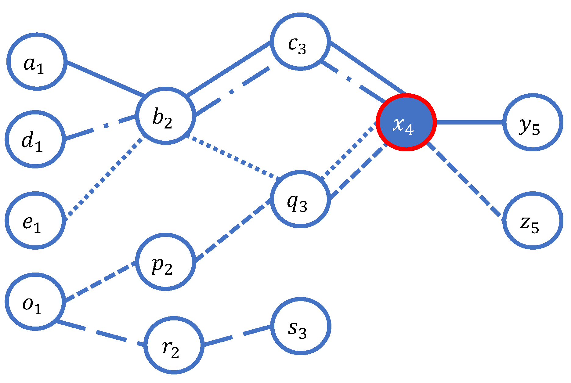
Figure 2.
The graph of the users’ visited sequence locations.
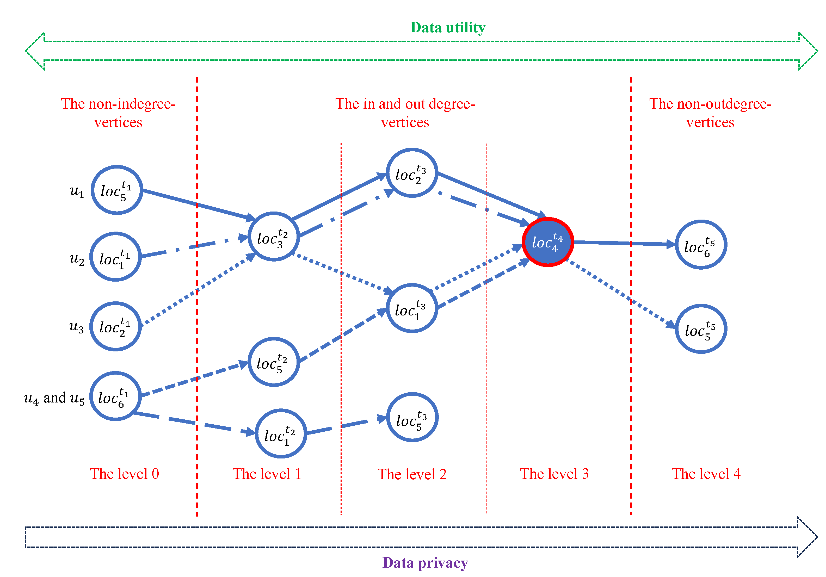
Figure 3.
An example of R-Trees.
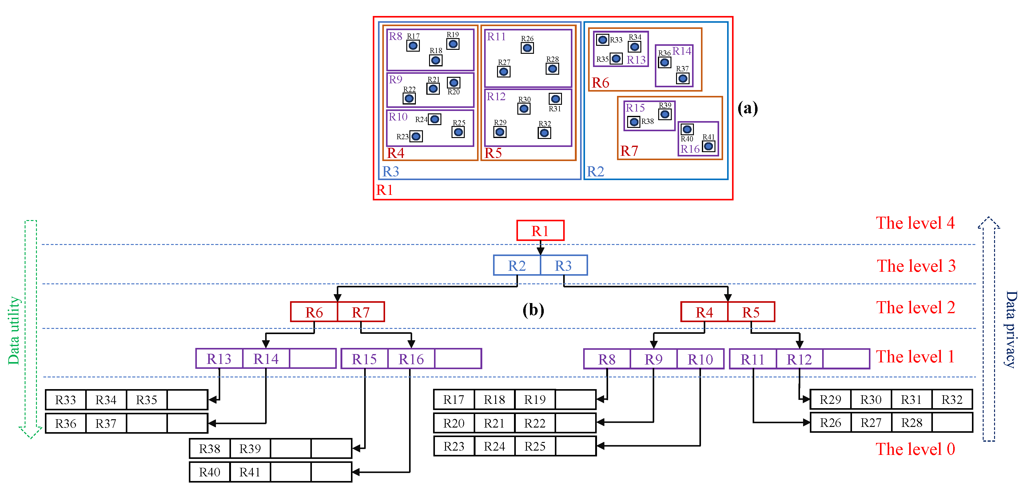
Figure 4.
Four data versions of Figure 2 are after suppressing the vertices of levels 1, 2, 3, and 4, respectively.
Figure 4.
Four data versions of Figure 2 are after suppressing the vertices of levels 1, 2, 3, and 4, respectively.
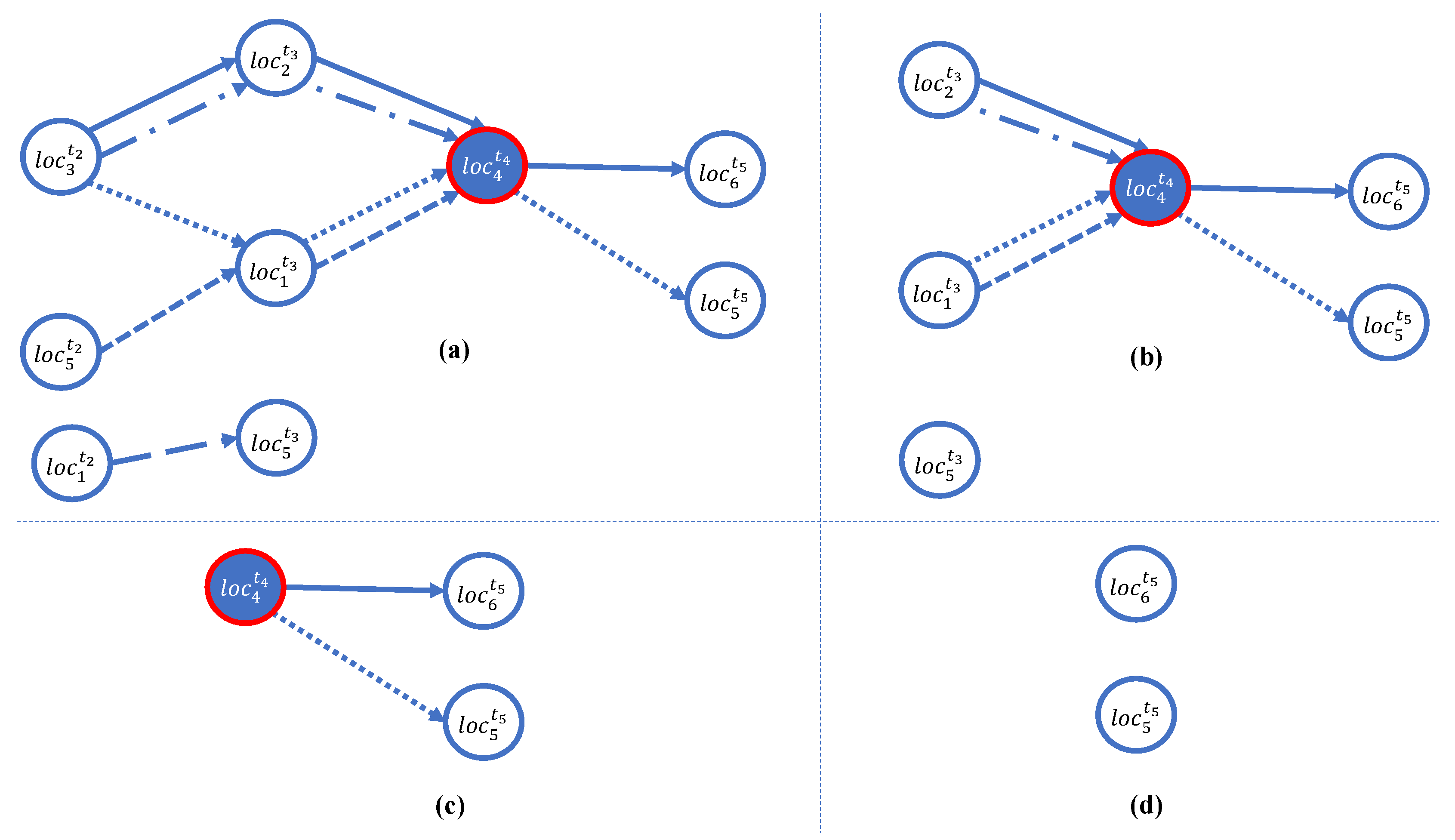
Figure 5.
The characteristic of bounding the locations with Split-Halves R-Trees.
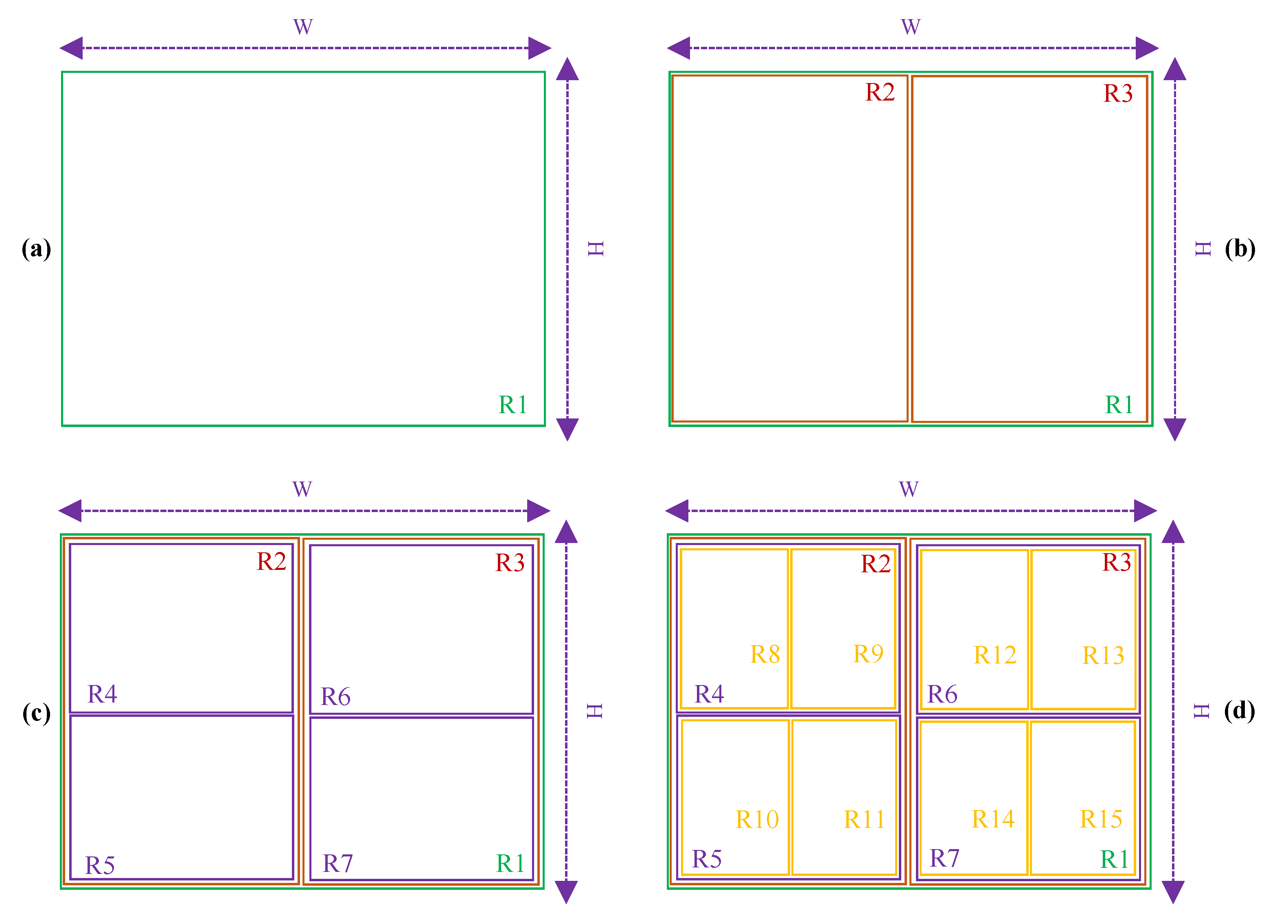
Figure 6.
Effect of the , , , and dataset size on the utility loss.
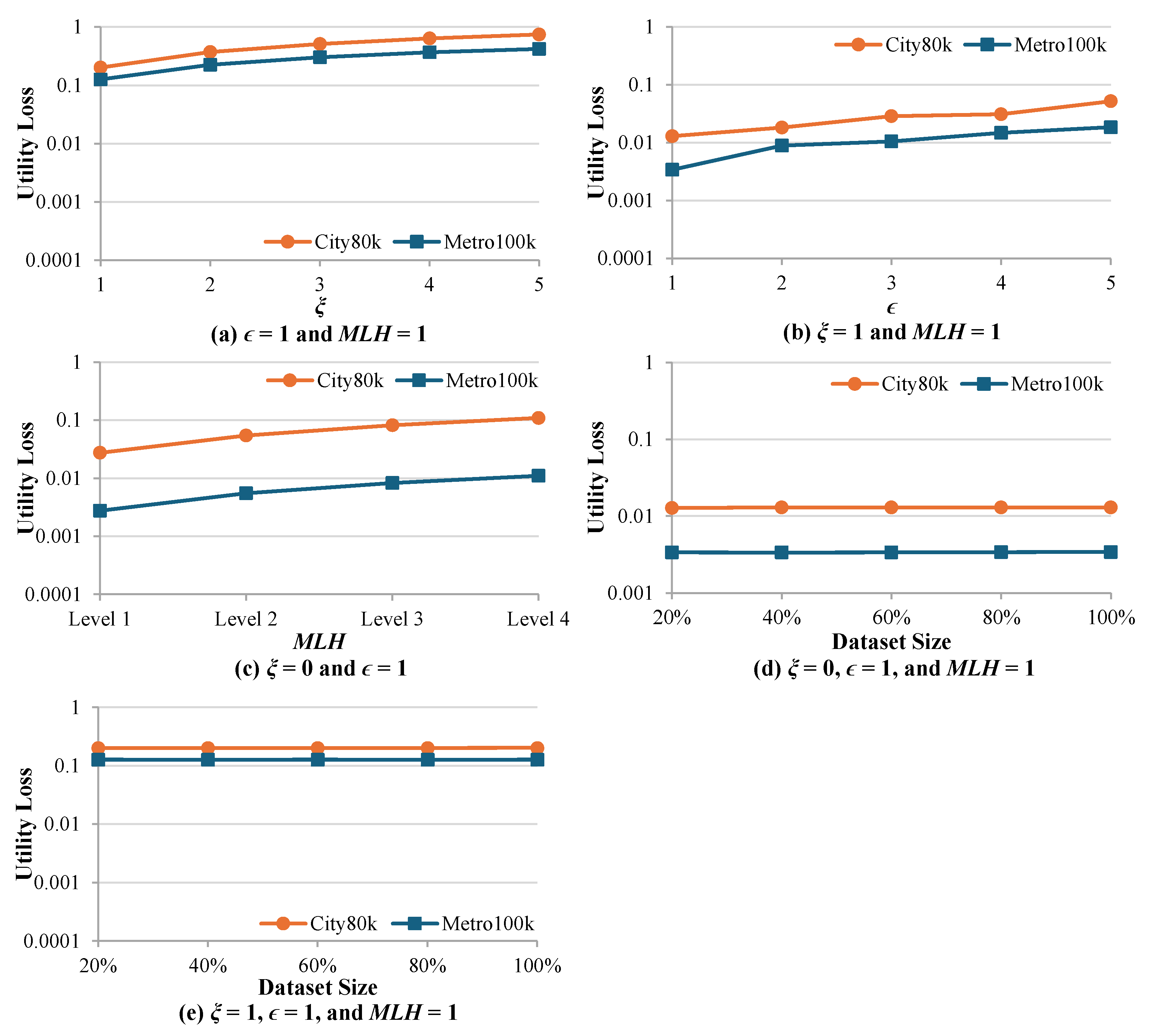
Figure 7.
Effect of the , , , and dataset size on the execution time.
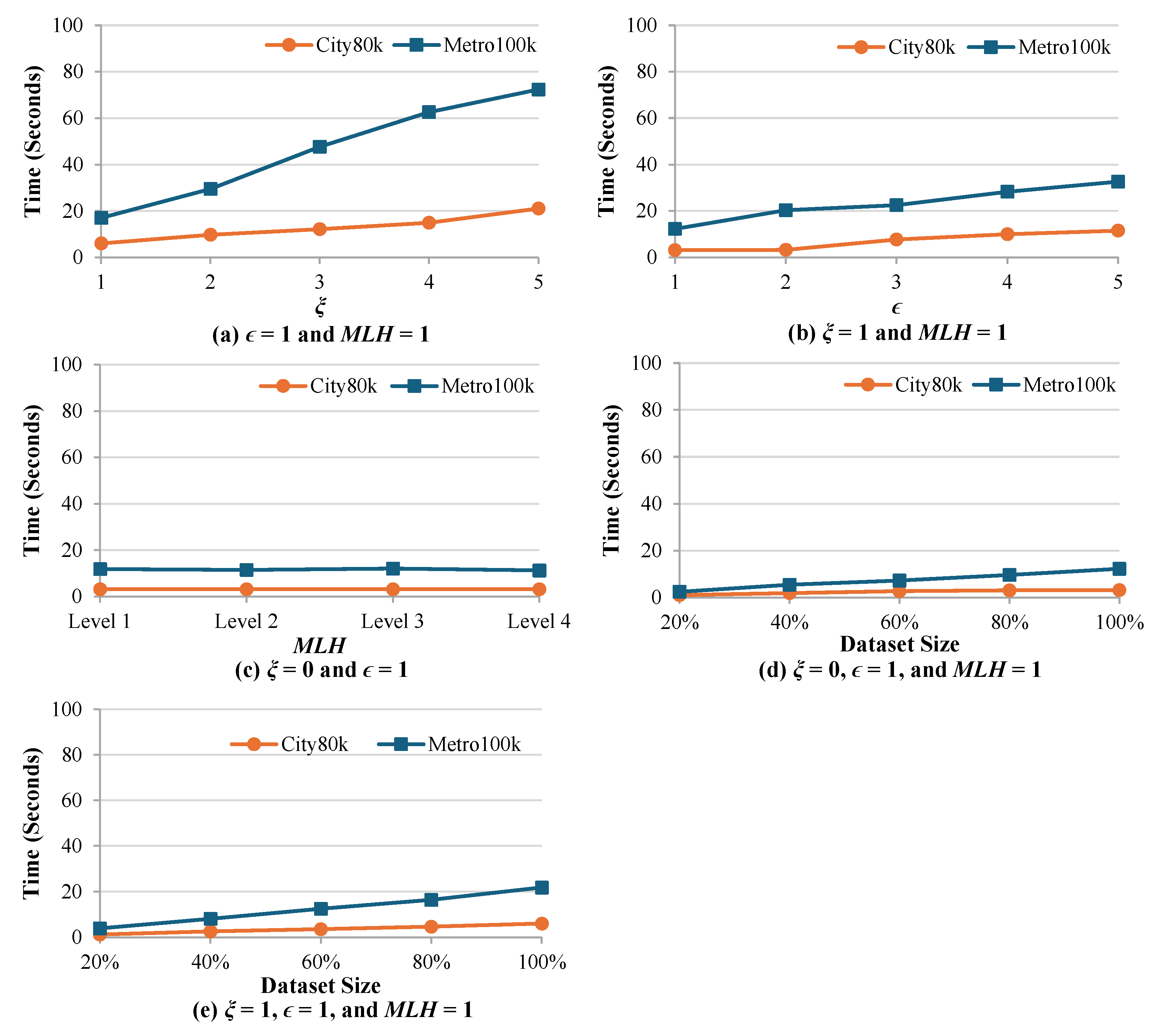
Figure 8.
Effect of the relative error across query types.
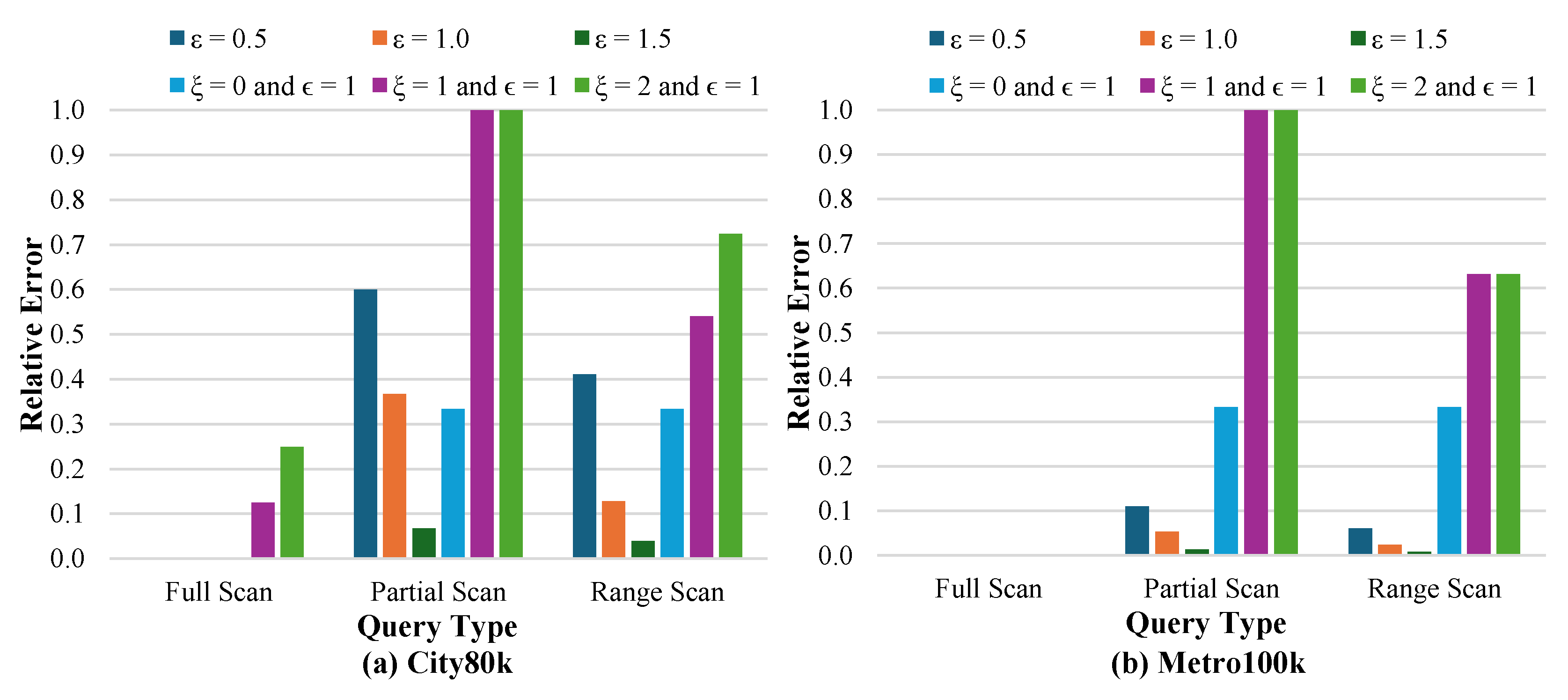

Table 1.
An example of trajectory datasets.
| Path | Diagnosis | |
|---|---|---|
| HIV | ||
| Food poisoning | ||
| Leukemia | ||
| Gerd | ||
| Cancer | ||
| Flu | ||
| Diabetes | ||
| Tuberculosis | ||
| Conjunctiva | ||
| Flu |
Table 2.
A data version of Table 1 is satisfied by LKC-Privacy constraints, where L = 2, K = 2, and C = 0.70.
Table 2.
A data version of Table 1 is satisfied by LKC-Privacy constraints, where L = 2, K = 2, and C = 0.70.
| Path | Diagnosis | |
|---|---|---|
| HIV | ||
| Food poisoning | ||
| Leukemia | ||
| Gerd | ||
| Cancer | ||
| Flu | ||
| Diabetes | ||
| Tuberculosis | ||
| Conjunctiva | ||
| Flu |
Disclaimer/Publisher’s Note: The statements, opinions and data contained in all publications are solely those of the individual author(s) and contributor(s) and not of MDPI and/or the editor(s). MDPI and/or the editor(s) disclaim responsibility for any injury to people or property resulting from any ideas, methods, instructions or products referred to in the content. |
© 2025 by the authors. Licensee MDPI, Basel, Switzerland. This article is an open access article distributed under the terms and conditions of the Creative Commons Attribution (CC BY) license (http://creativecommons.org/licenses/by/4.0/).
Copyright: This open access article is published under a Creative Commons CC BY 4.0 license, which permit the free download, distribution, and reuse, provided that the author and preprint are cited in any reuse.


