
Submitted:
26 August 2025
Posted:
27 August 2025
You are already at the latest version
Abstract
Ocean heat content (“OHC”)—the heat energy within the ocean integrated to a reference depth—has physical drivers spanning spatial and temporal scales, including seasonality, El Niño / Southern Oscillation (ENSO), and others. The present article investigates changes in OHC100 during the period 1994-2020 using GLORYS12 monthly-averaged ocean reanalysis. OHC100 – ENSO correlation patterns are explored to glean insights about the oceanic mechanisms that facilitate ENSO’s global teleconnections. After extracting known seasonality and ENSO signals using the Oceanic Niño Index (ONI), the OHC100 residual is analyzed to investigate multidecadal drivers of OHC100. Lagged ENSO – OHC100 correlations (±12 months) reveal basin-scale oscillations in the sign of ENSO influence likely attributable to Rossby waves. OHC100 is increasing globally (in total 2.4x10²² J decade-1), with greatest increases near western boundary currents (WBCs). Some regions are decreasing, notably the Atlantic Main Development Region (MDR) for tropical cyclones (TCs). Correlations and multidecadal variability in the OHC100 tendency (OHCT) and zonal and meridional advections of OHC100 (ZAO and MAO) support the hypothesis that upper-ocean dynamics mediate ENSO teleconnections as well as exert an independent control of OHC100 variability. Local increases in OHC100 would support observed TC rapid intensification irrespective of ENSO phase as the TC-supporting region expands.
Keywords:
tropical cyclones
; El Niño – southern oscillation
; multiscale dynamics
; upper ocean heat content budget
; global teleconnections
; rapid intensification
1. Introduction
It has long been established that because the Earth system is not in local thermal equilibrium, there is a complex transport of heat from the equator to the poles that establishes global (systemic) thermal equilibrium [1]. Geologically recent changes in the Earth system have led to greater temperatures in the ocean [2,3] and atmosphere [4]. Because the ocean has a much higher heat capacity than the atmosphere [5], 93% of the energy responsible for warming the Earth works to warm the ocean [6]. Hence, the ocean has a strong regulatory effect on the Earth system temperature, and its heat content is of considerable scientific and practical interest.
Thermodynamic ocean feedbacks to the atmosphere act mainly via ocean heat content (OHC) (an energy source) and sea surface temperature (SST) (which regulates the rate of heat exchange between ocean to atmosphere). OHC is well-studied, with several landmark papers quantifying the amount of heat within various depths of the ocean using remote sensing datasets [7,8] as well as ocean reanalyses [9,10]. Global, gridded, physically consistent reanalyses are ideal for studying global patterns on multidecadal timescales. One major area of inquiry regarding effects of multidecadal global ocean temperature change is in the frequency, distribution, and intensity of tropical cyclones (TCs). TCs are known to derive their energy source from the warm ocean, and the impact of observed ocean warming on the TC characteristics is complex and multifaceted. This is due to feedback mechanisms between the ocean and atmosphere acting across spatiotemporal scales, which may amplify or diminish TC characteristics circumstantially. For instance, positive ENSO phase (“El Niño”) is associated with ocean warming, which increases the availability of heat to drive TCs, but also increases vertical shear of horizontal wind, which is detrimental to TC intensity on large spatiotemporal scales. The unexpectedly active TC seasons during the El Niño of 2023 highlights the challenge of predicting the outcome of these competing factors [11,12]. In contrast, recurrent mesoscale warm core ocean eddies or marine heatwaves (MHWs) may amplify OHC and drive TC intensification locally without the same negative feedback as positive ENSO phase.
The complexities of these processes are not sufficiently described by SST alone [13]. Supporting evidence so far indicates that the thermal influence of the ocean on weather is limited to within about 300 meters of the ocean surface [7], rather than depths of 300-2000 meters [6,9] or whole ocean depth to which OHC is sometimes calculated for analysis of Earth’s energy budget. MHWs are sometimes quantified using the heat content of the top 50 meters [14] and arise both from heating of the ocean and OHC convergence. Mesoscale ocean eddies frequently have a strong core in the upper 100m but not at the surface [15]. Physically, this means that only the near-surface ocean can interact with the atmosphere on spatiotemporal scales associated with weather (about 100 meters deep [16]). However, this relationship can be circumstantially perturbed by ENSO, confounding attempts to study the long-term changes in 100-m OHC (OHC100). Yet, there has been no attempt to remove the ENSO signal from OHC100 to better understand the future implications for extreme weather potential. With these observations in mind, this study seeks to establish OHC100’s relationship to ENSO (i.e., correlations) and its multidecadal changes (i.e., non-ENSO residual) with commentary on implications for TCs.
A rich body of literature has emerged aiming to determine the magnitude and predictability of TC characteristics and their oceanic and atmospheric drivers, including ENSO. This literature has largely addressed SST, OHC, ocean circulation, and the frequency, duration, intensity, and size of TCs. Kortum et al. [17] investigated the relative roles of SST-forced changes and weather variability in driving shifting Atlantic TC tracks and frequency. They made a case for a substantial “weather”-driven component to changes in TC distribution and noted that internal climate variability (i.e., ENSO) exerted little control, emphasizing a need to understand local factors influencing TC genesis location [17]. That paper was motivated by observations that TC frequency has increased and shifted geographic distribution in the North Atlantic during 1970-2021; however, Chand et al. [18] found that TC frequency has decreased globally and regionally relative to the pre-industrial era (during the 20th century), consistent with the argument that large-scale warming weakens atmospheric circulation and suppresses TC formation. The evaluation of changes in TC frequency is sensitive to the selection of timeframe, geographic region, and variables under consideration. Feng [19] analyzed Western North Pacific TC translation speed during 1980-2023 and found that 80 km decade-1 poleward migration of TCs increased the basin-wide translation speed by 5% (due to beta effect) but regionally an 18% slowdown occurred. This study accounted for the effects of ENSO by performing their statistical analysis on non-ENSO residuals under assumption of time-stationary teleconnections. The TC slowdown and poleward migration are plausibly linked to the same underlying SST warming and feedbacks to atmospheric steering flow, and increasingly favorable conditions for TC maintenance [19]. Li et al. [20] examined rapid intensification (RI) in coastal regions (as opposed to the deep ocean where historical TC intensity studies have mainly focused) and found that RI events have significantly increased in frequency and moved landward during 1980-2020, driven by intensification-favorable ocean conditions. This study also accounted for ENSO by removing its influence from SST time series before statistical analysis. Of the important factors, relative humidity and vertical wind shear were more favorable near the coast than in the open ocean, whereas TC potential intensity (PI) increased uniformly across most of the global ocean and was a dominant factor for RI [20].
PI is a theoretical measure that prognosticates the strongest wind speed a TC could attain under given atmospheric and oceanic thermal conditions. PI has received considerable attention as a means to predict and identify spatial patterns in TC intensity [13,21,22,23,24,25,26,27,28,29,30,31]. Current methods of calculating PI focus on SST, although it is known that subsurface ocean structure can impact TC intensity immensely [32,33,34,35,36,37,38,39] and that depth-integrated temperature metrics, like OHC, can be better predictors than SST [40]. Shifting TC prevailing tracks can strongly impact how nonuniformly distributed factors change TC intensity, such as by sending TCs into higher-PI regions [41]. Potential intensification rate generally follows the distribution of PI [20]. Deshpande et al. [42] found that increased SST and tropical cyclone heat potential (TCHP, one measure of OHC) supported increasing intensity and frequency of strong TCs in the Arabian Sea and Bay of Bengal. Vidya et al. [43] found that both local oceanic factors such as OHC300 (i.e., OHC integrated to 300-m depth) and remote northern high-latitude influence on atmospheric upper-level vorticity and vertical shear were important for TC genesis in the Arabian Sea. Free et al. [13] pointed out that reanalysis of PI during 1975-1995 overstated increases in PI relative to 14 tropical island locations that exhibited no significant multidecadal change; however, both reanalysis and the radiosonde-derived PI showed similar likely ENSO- and SST-driven interannual variability. During 1975-1980 SST increased and PI decreased, illustrating a need to predict changes in TC intensity from more than just SST [13]. Despite the apparent mismatch between implementations of PI in reanalysis and observations, estimation of PI from thermodynamic principles remains desirable due to challenges measuring and forecasting actual intensity changes. These research efforts collectively call for deeper exploration of how the OHC that interacts with the atmosphere to directly or indirectly influence TC geographic distribution, genesis and intensification.
Past efforts to take stock of changing upper ocean OHC [6,7,9] have generally conducted the analysis without disaggregating the large, well-known ENSO signal from residual non-ENSO changes. Johnson & Lyman [6] examined the global patterns in observed 700-m OHC for the period 1993-2019 and found that 56% of the global upper ocean area is significantly warming and 3% is significantly cooling. Local values of the change over 27 years from -8 to 7 Wm-2 which is much larger than the global average, 0.60 Wm-2 [6]. The global heating they calculated was equivalent to 0.42 Wm-2 over the Earth’s entire surface during the study period [6]. This evaluation of historical changes demonstrates the dominant ocean warming pattern but does not address the degree of command that ENSO exerts versus unquantified effects. Cheng et al. [9] examined OHC100 and associated heat fluxes under varying ENSO conditions, confirming strong diabatic negative OHC tendency (that is, flux of heat stored in the ocean to the atmosphere) during positive ENSO phase, as well as vertical and horizontal redistribution of OHC100. The presence of transitions between positive and negative correlation with ENSO at various lag times was apparent in their results but not discussed. Their results excluded the regions poleward of 60° and did not address what residual if any there was when the ENSO signal is removed. Xu et al. [44] addressed global change in ocean temperature from the standpoint of MHW occurrence and found that MHWs evident in SST increased almost worldwide due to local effects rather than ENSO during 1958-2017 in observations and CMIP6 historical simulations. Understanding the changes in the residual is as essential for anticipating future changes to the global system as changes in ENSO. Since temporal variability is much greater at local than global scales, the more granular the assessment of these changes, the better the representation of dynamic regions like western boundary currents (WBCs) and shallow coastal regions. Deciphering the relative contributions of ENSO and residuals to OHC100 can support conclusions about future impacts on TCs.
On larger spatiotemporal scales, ENSO is associated with a strong redistribution of OHC, either through a direct influence as in the Pacific Ocean [45] or via teleconnections globally [46]. Cooling of the ocean and atmosphere occurs globally during and after El Niño events [9], although the exact mechanism [be it the “delayed oscillator”, “recharge-discharge oscillator”, “western-Pacific oscillator”, or “advective-reflective” paradigm] and timescale by which ENSO impacts OHC are not fully understood. The delayed oscillator model formalizes the way in which Rossby waves and returning Kelvin waves could be involved in generating low-frequency oscillations associated with ENSO [47]. The recharge-discharge oscillator model emphasizes the importance of building and dissipating OHC [47], a process largely mediated by OHC tendency (OHCT) and meridional advection of OHC (MAO). The advective-reflective oscillator model was inspired by observations of reflecting equatorial Rossby and Kelvin waves and their associated zonal advection of OHC (ZAO) impacts [47]. Naturally, these factors are all represented in the unified ENSO oscillator model, of which the former models are all special cases. A substantial fraction of Earth’s ocean and atmosphere variability is explainable by correlation with ENSO—even at timescales shorter and longer than the well-known 2-7 year ENSO cycle timeframe [48]. Additionally, ENSO is asymmetric with respect to its positive (El Niño, warmer Pacific) and negative (La Niña, cooler Pacific) phases [49,50,51]. The broadband and asymmetric nature of ENSO contributes to the fundamental mystery of how it interacts with drivers of long-term background changes (henceforth “residuals”). This interaction may determine whether changes in ENSO and residuals have positive or negative impacts on features of the global Earth system, including extreme weather. Changes in the ENSO-driven and residual component of OHC have ambiguous impacts on frequency, intensity, and other characteristics of TCs, which arises from a few sources.
First, the determination of an El Niño or La Niña event via an exceedance threshold of i.e., the Oceanic Niño Index (ONI) suffers from the fact that ENSO [52,53] and ocean temperature in general are statistically nonstationary. The occurrence of any threshold value drifts over time as the mean changes and because autocovariance depends on choice of time interval. This makes attribution of changes in e.g. frequency of extreme weather events due to ENSO or residual effects problematic—the meaning of ENSO changes over time. Second, the scale at which changes occur has meaningful impacts on extreme weather characteristics. Global changes in temperature may be classified as “Niño-like” (warming) or “Niña-like” (cooling) if they follow spatiotemporal patterns similar to ENSO [54]. It has been proposed that historical external forcing, if it were to continue, would lead to more Niño-like conditions [55]. However, local drivers of change may not merely add to the ENSO-like conditions imposed by the global changes. For instance, local changes in temperature or heat fluxes may lead to changing local support for extreme weather but may not have other features associated with large-scale dynamics such as impacts on vertical shear of horizontal wind. An example of a physical process that acts in this way could be mesoscale ocean eddies, which have been shown to impact occurrence of MHWs independently of global drivers [56]. A third source of ambiguity derives from the fact that ENSO impacts may occur with a lag an order of magnitude larger than the timescale of extreme weather (e.g., months earlier or later) and be facilitated by teleconnections [57,58]. When this is the primary mechanism connecting ENSO to extreme weather in a region, establishing the magnitude and significance of the relationship can be challenging to differentiate from natural variability or changes in the residual, even when equipped with a long time series. These issues are addressed in the present study by separating ENSO from residuals and examining their impacts separately, with attention to the scale of features and likely physical drivers.
2. Materials and Methods
2.1. GLORYS12 Monthly Average Ocean Reanalysis and ENSO Index
The ocean reanalysis GLORYS12 provides the geophysical variables on mean-monthly scales. GLORYS12 is a global eddy-resolving physical ocean and sea ice analysis having 1/12° x 1/12° horizontal resolution and covering the period 1993-present (of which we use the period 1994-2020) [59]. GLORYS12 is regridded bilinearly upscale onto a 0.5° x 0.5° monthly-averaged grid. The Oceanic Niño Index 3.4 (ONI) was obtained from the National Weather Service website [60]. ONI will be referred to as “ENSO” for sake of simplicity since it represents the SST anomaly in the Niño 3.4 region on which the prevalent ENSO indices are based. GLORYS12, like other reanalyses, has inherent biases with respect to its representation of e.g., ocean temperature [61]. Nevertheless, because of the fair agreement with other reanalyses and the fact that fixed biases are unimpactful on residuals calculated for the present analysis, GLORYS12 serves as a suitable proxy for a global gridded observational dataset.
2.2. OHC100, Its Time Tendency, and Horizontal Advections
OHC100, the total OHC above the 100-m isobath, is integrated from the base vertical level closest to 100 m to the surface – in the deep ocean regions of the GLORYS12 reanalysis, this is typically 112 m depth, and in shallow coastal regions, it can be shallower than 100 m. OHC100 advection that acts on the ocean-atmosphere heat budget is calculated by combining the OHC100 with ocean velocity fields and presented in its zonal (ZAO) and meridional (MAO) components. ZAO and MAO convergence can lead to accumulation of heat and impact air-sea interactions. The OHC100 tendency (OHCT) is calculated as a centered difference of OHC100 with respect to time. All three of these OHC100 budget terms (collectively “budget terms” henceforth) have units of heat flux (Watts per square meter). It is important to keep in mind that OHCT is positive (negative) when flux is into (out of) the upper 100 m of the ocean by convention. OHCT fluxes are generally between the ocean and atmosphere although it is possible that some component of the flux is across the base of the upper 100-m region for which it is calculated. Positive OHCT can be regarded conceptually as the “temporary storage” of heat in the ocean, and negative OHCT as flux to the atmosphere available to drive atmospheric dynamics such as TCs. OHCT has the opposite impact on heat available to the atmosphere compared to ZAO and MAO of the same sign.
2.3. Quantifying Correlations, Residuals, and ENSO Impacts
The influences of known signals—the seasonal cycle and ENSO, which vary in space and time—can be disaggregated from the remaining short and long-term residuals with standard signal processing techniques. While the seasonal cycle has some nuance due to its spatial variation, it is not the focus of the present study; it is removed by calculation and subtraction of the monthwise mean (e.g., mean of all January timesteps at each latitude and longitude—call this “deseasonalization”). Similarly, the ENSO contribution to any variable in question can be removed using its statistical relationship with the ONI. The ONI is calculated based on a lagged climatology and therefore possesses a bias towards El Niño conditions due to a warming climate [62], but it is the simplest reliable method to quantify ENSO for the signal processing performed here.
Correlations with ENSO and residuals for OHC100, ZAO, MAO, and OHCT are computed for the study period 1994-2020 and examined as spatial maps. The convention is to call correlation at n months of lag “lag n correlation”. The lag 0 correlation illustrates the relationship between the time series of ENSO and OHC100, OHCT, ZAO, and MAO in their respective subplots during the month when ENSO phase and observed data occur. This is in contrast with negative lag correlations (lag -12 to lag -1 correlations) for which data occur before ENSO, and positive lag correlations (lag +1 to +12 correlations) for which data occur after ENSO. While a strong correlation need not suggest a causal relationship between ENSO and a given variable, a strong correlation is often a consequence of causal links. It is reasonable to interpret low correlation as a non-causal relationship at the given lag—this does not preclude a strong correlation from occurring at a different lag and should not be generalized for all lags including those outside of the scope of this study. However, it should be noted that significant correlation is more difficult to establish at greater lag times since the number of degrees of freedom to work with decreases with increasing lag. With 324 months (27 years) of GLORYS12 monthly averaged ocean reanalysis, the number of degrees of freedom is 324 – 2 = 322, which for a two-tailed t-test with a significance level α = 0.05 (T ≈ 1.968) implies that in general, r-statistics with magnitude greater than 1.968([1.9682 + 322]1/2)-1 = 0.109 are significant on all correlation plots in these results. For the ±12 lag correlations, it is necessary to use 24 fewer months to properly align ONI and data, in which case the significant r-statistic magnitude is 0.113.
Penland and Matrosova [52] as well as Compo and Sardeshmukh [63] provided concise explanations of the difficulties surrounding ENSO removal and a critique of the regression method utilized here. The present study benefits from the perceived disadvantages of quantifying ENSO with regression since the spatial correlation maps can be examined through the lens of how ENSO signals propagate in lag space under the assumption of linearity. Some components of ENSO and the residual are intertwined (viz. nonlinear), with different frequency components of the ENSO influence peaking in correlation at different lags [48,49,52,53,63]. Hence, it must be kept in mind that the correlations should be read as “the linear correlation with Niño 3.4 region SST from lag 0 with the state at each spatial coordinate at the current lag”. It should also be kept in mind that the residual represents “the change of the component of the variable in question that is, conservatively speaking, not related to ENSO or seasonality”, knowing that the true change may be enhanced by nonlinear interactions with ENSO. Our correlation analysis focuses on lags ±12, spanning the timescale for which significant correlations are known to exist (for instance a couple seasons later in the Atlantic [64]). We avoid the difficulties associated with empirical orthogonal function (EOF) analysis and Fourier frequency filtering, since we hypothesize that dynamic aspects of ENSO (i.e., dipole and higher harmonic modes of ENSO variability that are necessary for observed signal spatial propagation to exist) and residuals are important for effects on TCs. The ENSO regression method for examining residuals has been justified in multiple publications [54,65].
3. Results
This section first demonstrates the importance of disaggregating ENSO from residual signals using TCHP before examining OHC100’s relationship to ENSO and the multidecadal changes in the non-ENSO residual. These research objectives introduced in Section 1 are framed with two research questions regarding ENSO-driven and residual-driven components of OHC100 in subsections 3.1 and 3.2. Detailed examination of OHC100, OHCT, ZAO and MAO correlations with ENSO is organized by ocean basin within 3.1. These results are contextualized with implications for TCs in Section 4, which separately considers where ENSO and residuals dominate, respectively, in subsection 4.1, and how these results impact TCs and extreme weather more broadly in subsection 4.2.
Disaggregation of ENSO and residual influences on OHC100 is essential for identifying how OHC100 has changed and may evolve in the future. The strong influence of ENSO on TCHP illustrates this well. TCHP has been a popular metric for OHC historically and long regarded as a natural metric to study ocean impacts on TCs. The justification for this metric has been the observation that TCs tend to intensify over waters warmer than 26°C [66,67,68]. However, more recent research has revealed that this threshold is a non-mandatory condition for TC maintenance and intensification [69]. Despite this shortcoming, TCHP has a stronger relationship with TC intensity than does SST [40]. The area of the TCHP region increased on average over 22,000 km2 annually during the period 1994-2020 (Figure 1a) concurrent with a prevalently positive change in TCHP magnitude in the same period (Figure 1b). The mid-latitudes to the poles experience less intense solar radiation and therefore cooler climatological ocean temperature and a smaller ≥26°C area. Waters warmer than 26°C expanded from the tropics towards the poles during the 1994-2020 study period. Periods of expansion and contraction largely coincide with transitions in sign of ENSO phase, superimposed on a long-term change associated with the residual. Figure S1 illustrates how the TCHP correlation with ENSO is still strong at the edges of the TCHP-defined region post-removal since the region is often larger (smaller) in positive (negative) ENSO phases. Figure S2 shows how the frequency with which TCHP exceeds zero varies with latitude. The effects of ENSO can be treated consistently for a fixed OHC integration depth and no threshold temperature as with OHC100.
3.1. How Do ENSO Correlations of OHC100, ZAO, MAO, and OHCT Change from ±12 Months Lag Globally at the Mesoscale?
Figure 2 depicts lag-0 ENSO correlation with OHC100, OHCT, ZAO, and MAO. Strong (|r| > 0.25) and significant (|r| > ~0.1, see Section 3.3) correlations occur for all four variables. OHC100 (Figure 2a) has significant correlations nearly globally, whereas OHCT (Figure 3b), ZAO (Figure 2c) and MAO (Figure 3d) are significant exclusively within 20° latitude of the equator. None of the variables exhibited features identifiable as WBCs, which appears to contradict previous literature finding strong ENSO signals in WBC strength [70]. Features likely associated with propagating equatorial Rossby waves (dispersive, propagate westward along the thermocline) and Kelvin waves (non-dispersive, propagate eastward along the thermocline about three times faster than Rossby waves) were apparent. Evidence of equatorial features agrees well with proposed ENSO mechanisms.
Transition zones between positive and negative OHC100-ENSO lag 0 correlation (Figure 2a) are a notable feature that has been evident in previous studies without discussion [9,71]. This transition zone must occur due to the continuous nature of the r-statistic, under circumstances where two variables can have changing sign of correlation. However, its coherence is not enforced in any way—it could very well have been an incoherent transition from one sign to the other, but this is not the case. Approximately zero correlation occurs in a strip usually oriented north-south with sub-basin-scale east-west meanders, a few hundred kilometers across; the approximate positions of these features are marked with solid lines (Figure 2a). The transition zones remain coherent and evolve at the various lags studied (Figure 3). Lags ±1, ±3, ±6, ±12 are shown in Figure 3, and all lags showing the temporal continuity of these patterns are available in the Supplementary Material (Figures S3-A7). The transition zones are sharper around lag 0 than at ±12 lag (Figure 3) but remain evident across the lags examined (Figure S3). Considering transition zones one-by-one in the Pacific, Indian, and Atlantic Oceans, some patterns of changing position, sign, and intensity in lag space emerge.
In the Pacific Ocean, the peak positive correlation of OHC100 and ENSO moves from northeast and west Pacific regions at lag -12 to the equator at lag 0, then reverses direction, precessing around the continental and equatorial margins of the North Pacific. The eastward propagation from lag -8 to lag 0 and poleward redistribution at positive lags described by Trenberth [72] is evident in Figure 3. This is consistent with the adiabatic horizontal redistribution of OHC by the recharge-discharge mechanism. A negative correlation in the west Pacific grows from -12 to the peak at +3 concurrent with the eastward movement of a region of positive correlation in the South Pacific. The Indian Ocean has positive correlations generally when the equatorial Pacific does (and vice versa) although they are weaker signals. Lag +12 shows weak correlations of both signs at all locations; this is likely due to the myriad known dynamical factors controlling Indian Ocean OHC100. Tropical Indian Ocean SST is known to show basin-wide warming about six months after positive ENSO, and is called the Indian Ocean basin (IOB) mode of the Indian Ocean SST interannual variability [73]. The triggering of downwelling Rossby waves by anomalous easterlies [74] is a likely mechanism by which correlations propagate at positive lag times. There is also evidence that meaningful correlations with ENSO can persist until lag +12 in the Indian Ocean: Rossby waves can lead to weakening of the southwest monsoon a year later in the summer [75] and hence positive wind-evaporation-SST feedback [76], warming the whole basin. The basin-wide oscillation is evident in SST lag correlation with ENSO (Figure S4). The IOB persists from boreal winter to the following summer despite dissipation of the positive-ENSO-related SST anomalies in the central and eastern Pacific [51]. The Atlantic Ocean signals are weaker than in the other basins but are usually negatively correlated at negative lags and positively correlated at positive lags. The gradual increase in correlation with ENSO at positive lags in the Atlantic is consistent with the documented anomalous post-positive-ENSO Atlantic warming and post-negative-ENSO Atlantic cooling [77].
The unified oscillator model of ENSO predicts that the physical processes that regulate ENSO are linked to ZAO, MAO, and OHCT. OHCT lagged correlations with ENSO (Figure 4) exhibit negative correlations with ENSO lock-step with OHC100 positive correlations on the same timescale. This matches the association of OHCT with off-equatorial discharge of accumulated OHC to the atmosphere, although OHCT still has strong ENSO correlations well outside of the tropics (Figure S5). ZAO and MAO relationships with ENSO (Figure S6-S7) are principally linked to equatorial wave processes and only weakly correlated at higher latitudes. One might imagine that OHC100 correlations should be a weighted average of the correlations of the mediating oceanic processes involved. However, it seems more likely that in regions where OHC100 correlation has a high R magnitude, but the mediating oceanic processes do not, ENSO impacts are mediated by atmospheric teleconnections that cannot be adequately resolved with ocean reanalysis alone. For instance, in the equatorial Pacific, it is known that surface wind mediates zonal transport directly or indirectly by triggering wave dynamics [78], but in off-equatorial regions, the direct impacts of surface wind-mediated processes that modulate OHC100 may not manifest as a coherent transport signal. In the equatorial Pacific, this may be related to the Madden-Julian Oscillation (MJO), an atmospheric disturbance that propagates eastward from the equatorial Indian Ocean to the Pacific Ocean on 30–90-day timescales. This manifests as strong correlations between ENSO and zonal and meridional ocean transport between the equatorial Pacific Ocean and Indian Ocean (Figure S10).
Away from the equator and in the Atlantic Ocean, the transition zones are better explained by changes in ocean temperature, likely induced by atmospheric changes attributable to ENSO (as opposed to, e.g., changes in the intensity of western boundary currents, which showed no significant correlation with ENSO). The substantial OHCT correlation at higher latitudes could be an indicator of atmospheric mediation. However, there are significant nontrivial differences between OHC100 correlations and SST correlations at the transition zones (Figure S8), confirming the importance of subsurface processes. Decoupling at even greater depths is expected to be greater, which agrees with results that suggested OHC2000 leading ENSO by a variable number of months between 1980-1999 [9]. Heat accumulates in the W. tropical Pacific during La Niña [79]. At negative lags, the W. tropical Pacific becomes increasingly polarized, with a sharp gradient from negative (west) to positive (east) correlation with ENSO arising. Simultaneously, the positive correlation intensifies and grows eastward, with the strong positive core eventually touching S. America at lag -1 and beyond. This is consistent with observed patterns [53,79,80,81]. The general reversal of patterns between negative and positive phase that sends heat back to the tropics resembles the diabatic heating impacts of the ENSO recharge phase, about which there are few publications [82,83] despite being an important aspect of frameworks explaining ENSO evolution.
3.2. What Does the Geographic Distribution of Residuals of These Variables Reveal about the Oceanic and Atmospheric Drivers of Change?
The OHC100 residual (Figure 5) is positive nearly everywhere with exceptions in the MDR, Agulhas Current, Niño 3.4 region, south of Greenland, around Antarctica, and a portion of the Kuroshio Current (Figure 5a). Skewness towards positive residuals and spatial patterns are similar to those in Johnson & Lyman [6] calculated for 1993-2019 and 700 m depth, but are significant over a greater area in this study—possibly due to the careful treatment of the ENSO signal. The greatest warming is poleward of 30°, however the equatorial region equatorward of 10° is warming everywhere except the Niño 3.4 region and a small piece of the MDR. In the Niño 3.4 region, the residual is expected to be relatively small since ONI is defined using this region and therefore ENSO should explain nearly all variability observed in that region. The residual there is nearly zero. Integrating the OHC100 residual over the area of Earth’s ocean yields a net warming rate of about 2.4x10²² J decade-1, which is comparable with the findings from 1993 to 2021 for the upper 2000 meters presented in Su et al. [8] calculated from other ocean models and remote sensing observations. When combined with the observation from Levitus et al. [7] that OHC below 300 m doesn’t substantially impact the global OHC variability, this indicates that most of the global OHC residual is represented in OHC100. However, this should not minimize the impact of warming at greater depths which is within an order of magnitude of the surface.
The decreasing OHC100 in the Irminger Sea (south of Greenland) likely reflects increasing loss of heat due to interaction with buoyant surface glacial meltwater—and not necessarily just from the southeastern fjords, because the Fram Strait delivers water to the region from virtually all of Greenland’s coast. Some component may also be attributable to observed Atlantic Meridional Overturning Circulation (AMOC) weakening since 2015 [6]. Correspondingly, decreases near Antarctica are likely related to meltwater entering the Southern Ocean. To our knowledge, the strong negative OHC100 residual near 10°N off the west coast of Africa has not been identified to date. This region is strongly impacted by Saharan dust, which impacts radiative forcing over the Atlantic Ocean [84] and leads to cooler SSTs [85,86] The shape of the region of decreasing OHC100 in the MDR matches the typical warm dry region circumscribed by a north-south oriented warm atmospheric ridge that results from Saharan dust [87]. If this similarity in shape of the OHC100 residual and the region impacted by dust is due to aerosol forcing, Saharan dust effects may have increased in intensity or frequency during the study period. This aligns with the finding of Miller & Ramseyer [88] that Saharan air layer outbreaks became 10% more common during 1981-2020. Figure S9 shows SST residual globally for comparison with OHC100 residual; in the MDR SST has a weaker signature than OHC100 which may have led this feature to be overlooked in previous studies. An additional factor that could have obscured this oversight is the fact that significant ENSO impacts on SST and OHC100 are in some regions including the MDR not in phase and can even have opposite signs (Figure S8). The quantified decoupling between the correlations of OHC100 and SST respectively with ENSO can be explained by the lead of shallow OHC100 ahead of SST development documented by Meinen & McPhaden [80]—however, the results here have a broader geographic scope than the central equatorial Pacific and in other regions SST may lead OHC100.
The MDR decreasing OHC100 region is not the only mesoscale feature apparent in the OHC100 residual: unlike the ENSO correlations in Figure 3, Figure 4 and Figure 5, WBCs and eddy-like features are apparent and dominate the areas with the largest residuals in addition to the equatorial wave-like features. Changes in basin-scale circulation have already been observed, with both poleward shift of global subtropical WBCs and warming of WBCs 2-3 times the global mean [89]. These features are even more apparent in the OHC budget term residuals (Figure 5b-d). In all three budget terms, the heat flux residuals are most pronounced at WBCs, the equator, and the ITCZ mean position. The residuals are weak at the highest latitudes where the ocean is frequently ice-covered.
It may be useful to think of the OHCT residual (Figure 5b) as the “acceleration of OHC100” during the 27-year period in question. OHCT residual is more negative (positive) with increasing (decreasing) flux to the atmosphere. All areas with negative OHC100 residual (Figure 5a) exhibit positive OHCT residual (Figure 5b), but the opposite is not universally true. In the Pacific, the band of locally elevated OHCT residual between 5-10°N coincides with positive OHC100 residual. The tropical Indian and Atlantic Oceans both exhibit an east-west basin-scale asymmetry with positive OHCT near Africa and negative OHCT elsewhere. At the poleward extensions of the WBCs, there is typically a greater occurrence of negative OHCT residual than near the tropical origins of the currents; the warming tropical ocean transports heat poleward via WBCs, which would lead to increased fluxes via OHCT to the atmosphere at mid-high latitudes.
Not all areas with large changes in ZAO and MAO residuals (Figure 5c-d) have similarly strong residuals in OHC100: this should be interpreted as changes in ocean circulation impacting transport of OHC100 more than the change of OHC100 itself. A nuance of advection residuals is that the sign convention, positive for east in ZAO and positive for north in MAO, leads to interpretation of increasing residuals as “more eastward” and “more northward” transport as well as “increasing magnitude”. That is, a negative residual may arise from a weakening or change of direction of flow. However, the direction of monthly average flow does not generally undergo reversals, so residuals should be interpreted as mostly attributable to changing magnitude. The greatest impact of flow reversal is likely in eddy-rich regions where changing mesoscale variability may lead to a dynamic ocean feature translating in space. As the ocean warms, there is more OHC100 to transport. ZAO and MAO can attain values of around 5000 W m-2 yr-1 in the areas of most intense increase. One possible explanation for the mesoscale structure of the residual maps is that there are variations in mesoscale dynamics on timescales similar to the length of the 27-year dataset. Thus, mesoscale eddy processes may transport long-term signals on a multidecadal timescale, localizing rather than diffusing changes in the system. Near the equator, the wave-like structure may indicate amplification of the OHC signal that the waves carry. These patterns can be attributed to two factors: increasing tropical OHC100 that is pumped poleward by the global thermohaline circulation, and movement of the western boundary currents. The former is a robust signal based on the global change in OHC100, whereas the latter is sensitive to the selection of analysis period, since the position of western boundary currents has substantial annual to multidecadal variability [90].
4. Discussion
4.1. Which Regions Are ENSO-Dominated, and Which Are Residual-Dominated?
Impacts of a changing upper ocean heat budget on TCs occur across spatial and temporal scales. ENSO has a global broadband signal that peaks on 3–7-year timescales, and long-term residuals with multidecadal timescales accumulate via changing dynamics that are most energetic at the mesoscale. These signals combine to dictate how the ocean drives TCs, controlling their thermal energy source and modulating the physical processes that shape their characteristics. ENSO exerts its strongest influence on the tropical Pacific, but ripples outward geographically and in lag space to have direct impacts and teleconnections globally. The results presented here support the various distinct ENSO models and the propagation mechanisms that they suggest, as well as their combination in the unified oscillator model. Wherever the magnitude of correlation with ENSO approaches unity, ENSO explains almost all variability, even on multidecadal timescales. Elsewhere, other factors that impact the residual are important. Disaggregating the influences of ENSO and residuals means identifying where the residual is important enough to reduce the ENSO correlation—at all lags. Observing that the WBCs, high latitudes, and shallow coastal regions both possess intense increasing OHC100 residual and a weak ENSO influence in general, these areas stand out as being controlled mainly by local non-ENSO processes. Over the course of years or decades, impacts on the order of ENSO-driven variations elsewhere may impact these regions. As for the other regions, the robust increasing residual over much of the world ocean would likely lead to more Niño-like conditions in the tropical Pacific as in Vecchi & Soden [91]. ENSO impacts the intensity and occurrence of extreme weather events including TCs [92], which is likely to intensify when the residual agrees in sign with the ENSO impact. This highlights the simultaneous importance of mesoscale features and the dominance of ENSO in these areas.
4.2. What Are the Implications for TCs and Other Extreme Weather?
It is important to determine what effect changes in OHC100 would have on the dynamics that control TC characteristics. For instance, vertical shear of horizontal wind (which is detrimental to TC formation and intensification) may only be impacted by large-scale changes in heating that occur on at least months-long timescales (ENSO-like), and could be unaffected by smaller or shorter scale heat flux changes (local), or vice versa. Using increasing temperature as an example, because most of the world is experiencing this type of change, there are two possibilities. One is that warming will lead to more positive ENSO-type conditions globally on average, and the diagnosed effects of positive ENSO phase on TCs will prevail, with less supportive atmospheric conditions but greater energy to drive storms that survive. The other possibility is that the greater energy source will persist, but because the mechanism is not ENSO-like, the negative feedbacks that would reduce TC intensity might not kick in, leading to a unilateral increase in TC strength if the pattern continues. In the latter case, increased latitudinal shear of ocean temperature and increased stratification work to increase TC-induced cooling and dampen TC intensification [93,94]. Geographic variation in ENSO strength opens the possibility of a mixed response, with some regions experiencing intensified ENSO-like variability and others experiencing mainly effects of the residual. Increases in conditions supporting TCs in the central Pacific could, via increased TC activity, result in increased transport of warm water to the cold tongue zone of the equatorial Pacific and promote El Niño conditions, as hypothesized by Fedorov [95]; in contrast, regions distantly impacted by ENSO via teleconnections like the N. Atlantic could experience TC intensification simply by merit of local heat flux changes.
A deep warm subsurface layer can directly enhance heat fluxes to the atmosphere under TC conditions [96]. Positive residuals of ZAO and MAO indicate increasingly favorable mean conditions for TC intensification. A warming ocean increases not only the heat available to TCs for intensification, but the temperature disparity between the surface and outflow level near the tropopause. This temperature disparity is a primary factor controlling TC intensity, so regions with increasing OHC100 are likely to see increasing PI as well. ENSO modulates TC activity worldwide [97], and patterns in ENSO lagged correlations may provide early indicators of TC activity when supportive ENSO phase coincides with TC season. For instance, OHC variability in the eastern Pacific Ocean is valuable for TC forecasting in the region [98,99], and this region regularly shows high correlation with ENSO. Similarly, correlations driven by teleconnections at greater lag times could provide some predictive capability on subseasonal timescales. Warming in inland seas such as the Mediterranean Sea may explain the recent increase in so-called “Medicanes” during the study period [100]. Local maxima in residuals may also explain recent increases in TC frequency in the Bay of Bengal relative to the Arabian Sea [42].
Marine heatwaves (MHWs) are a possible mechanism by which changing ocean temperatures force extreme weather across scales. MHWs originate and evolve under oceanic and atmospheric forcing. MHWs are often associated with ENSO [101], although there may be multiple mechanisms by which MHWs occur only some of which are related to ENSO. For those that are ENSO-related, it has been shown that MHW forecast skill can increase when models are initialized during El Niño [101] in areas that are highly correlated with ENSO. The importance of local versus remote dynamics on MHWs is a current area of research [56]. MHWs can increase in frequency even if local SST variability does not increase [44], which can be attributed to the importance of subsurface processes like ZAO and MAO convergence. Changing ocean conditions, whether due to ENSO or residual effects, may impact the prevalence or intensity of MHWs, with a cascade effect to the frequency or intensity of extreme weather. Increasing ZAO and MAO point to OHC100 convergence contributing to MHW intensity or occurrence; positive OHCT residual suggests increasing flux into the ocean and may support the idea that atmospheric forcing contributes to increasing MHW longevity in these regions [102]. Changes in MHWs have been hypothesized to feed back to TC rapid intensification in some regions [103], especially in shallow regions vulnerable to coastal downwelling during TC approach [34]. The ENSO correlation lag plots may indicate regions that could see MHW conditions months in advance. Positive residuals may also explain the recent normalization of historical marine heat extremes [2]; a shift of extreme conditions from relatively rare to common could result from global increases in OHC100, and increased occurrence of extremes could result from increased ZAO, MAO, and OHCT contributing to enhanced variance of OHC100. The locations of eddy-like features in the residuals may indicate where oceanic mesoscale eddies could be contributing to changes in MHWs [14].
PLs have dynamical similarities to TCs [104] that make many arguments applying to TCs also applicable to PLs in the context of ENSO and OHC100 impacts. In PL and TC literature alike, the thermodynamic disequilibrium between the surface (typically over the ocean) and the upper troposphere is used to evaluate environmental favorability for formation and intensification [105]. PI theory has likely not been applied to PLs to date because of conflicting conclusions about what controls PL intensity in the literature. However, it is important to separate conceptually the influence of ocean temperature on a particular PL from the influence of ocean temperature on PL occurrence and intensity on longer timescales. Warm WBCs are known to be important for TC intensification, but even at high latitudes they influence PL climatology [106]. Since the WBCs exhibit the greatest rates of increasing OHC100, which is related to SST, this is likely to drive up probability of formation of PLs in regions impacted by WBCs. Additionally, if PI theory applies to PLs as well as TCs, as has been hypothesized [104], these PLs may become more intense over time as well. SST anomalies may not significantly impact particular PLs but increased fluxes to the atmosphere due to ocean dynamics do create conditions favorable for PL intensification [107]. While, for PLs, positive SST anomalies may not increase the probability of PL formation as much as low air temperatures, SST has a controlling influence on where PLs may form [106]. MHWs also occur in regions that may be impacted by PLs in both hemispheres. For a particular subset of MHWs, those due to stationary zonal wavenumber-4 (W4) anomalies [108], the locations of the peak positive anomalies in the Southern Ocean—between Australia and Africa, central Pacific east of New Zealand, western Atlantic near the convergence of the Brazil and Malvinas Currents, and western Indian Ocean regions—saw local maxima in positive OHC100, ZAO, MAO, and OHCT residuals.
5. Conclusions
ENSO correlations of OHC100, ZAO, MAO, and OHCT change in lag space, reflecting the different speeds with which components of the complex ENSO signal propagate. Lagged correlations of OHC100 with ENSO show strong correlations even months before and after changes occur, perhaps revealing sources of predictability for OHC100 and its effects on TCs months in advance. The geographic distribution of residuals of these variables reveals not just increasing global OHC100, but increasing heat budget terms over much of the world ocean. This partitions the effects of a warming ocean into ENSO-like effects with competing feedbacks to TC characteristics and local effects that increase support for strong TCs. The large-scale ocean warming may drive more Niño-like conditions with possible feedbacks to the atmosphere that could suppress TCs such as increased vertical shear of horizontal wind and weakened large-scale circulation. However, more local features of the warming patterns may not contribute to ENSO-like feedbacks and may simply add to the energy source and thermal disequilibrium that drive TCs.
The tropics are ENSO-dominated, and the residual is important near WBCs, at high latitudes, and in shallow coastal regions. The hypothesized mechanisms of ENSO propagation in the ocean are well-represented in lagged correlations. While a substantial fraction of OHC100 is related to ENSO, the residual drives change on smaller spatial scales. Mesoscale processes and global ocean circulation are critical to the difference between ENSO impacts and residual impacts. WBCs have the most intense positive OHC100 residuals, which could have an intensifying effect on landfalling TCs in North America and Asia. Interannual variability of TC characteristics influenced by OHC100 may follow spatial patterns of ENSO correlation. Residuals will increase the availability of heat from the ocean to drive TCs even if unrelated ENSO feedbacks work to reduce intensity or frequency or change the geographic TC distribution. Intense and rapidly-intensifying TCs are likely to increase in frequency under the influence of increasing residuals, with MHWs serving as the mechanism that feeds ocean heat accumulation back to the atmosphere. The global changes in OHC100 and ocean dynamics may impact other forms of extreme weather as well, leading to changing frequency or intensity of PLs and explaining the rise of TC-like “medicanes” in the Mediterranean Sea. Ocean dynamics are important not just for mediating ENSO effects globally but for exerting independent control on local processes that feed back to TC intensity.
Future work could include:
- Incorporating analysis of atmospheric variables like surface and upper troposphere temperature and winds from a compatible reanalysis such as ERA5 could provide further insights into how ENSO-like or “residual-like” ocean-driven extreme weather impacts were during the study period—this would inform what these impacts would be like if they continued into the future;
- Confirm the symmetry of OHCT, ZAO, MAO responses to ENSO at various lags—since El Niño phase is known to last longer and have greater intensity than La Niña phase, correlations may disproportionately represent the former, but on the other hand, the correlations are fairly strong, which may support a symmetric response to both phases;
- Further investigation of OHC100 leading SST in correlation with ENSO and vice versa—does this relate to the local direction of forcing between ocean and atmosphere?
Supplementary Materials
The following supporting information can be downloaded at the website of this paper posted on Preprints.org.
Author Contributions
Conceptualization, R. K. Forney.; methodology, R. K. Forney; software, R. K. Forney; validation, R. K. Forney; formal analysis, R. K. Forney; investigation, R. K. Forney; resources, T. A. Smith; data curation, R. K. Forney; writing—original draft preparation, R. K. Forney; writing—review and editing, P. W. Miller and T. A. Smith; visualization, R. K. Forney; supervision, P. W. Miller and T. A. Smith; project administration, P. W. Miller and T. A. Smith; funding acquisition, T. A. Smith. All authors have read and agreed to the published version of the manuscript.
Funding
This work was funded as part of the US Naval Research Laboratory’s 6.1 Research Option “Interactive Relationships between atmospheric Convection and Subseasonal Oceanic Modes along the Equator” (IRCSOME).
Data Availability Statement
Data supporting this research are available in Jean-Michel et al. 202159. Datasets of e.g., OHC100, TCHP, etc., derived from these publicly available datasets and their generating software are available to researchers possessing a nondisclosure agreement and cooperative research and development agreement or via a licensing agreement with the U.S. Naval Research Laboratory.
Acknowledgments
The authors thank Adam Rydbeck and the IRCSOME project team members, Lew Gramer, Ghassan Alaka, Gregg Jacobs, Richard Allard et al. for their insights and encouragement.
Conflicts of Interest
The authors declare no conflicts of interest.
Abbreviations
The following abbreviations are used in this manuscript:
| ENSO. | El Niño – Southern Oscillation |
| ITCZ | Intertropical convergence zone |
| MAO | Meridional advection of ocean heat content |
| MDR | Main development region for tropical cyclones |
| MHW | Marine heatwave |
| ONI | Oceanic Niño Index |
| OHC100 | Ocean heat content of the upper 100 meters |
| OHCT | Ocean heat content tendency |
| PI | Tropical cyclone potential intensity |
| PL | Polar low |
| RI | Tropical cyclone rapid intensification |
| SST | Sea surface temperature |
| TC | Tropical cyclone |
| TCHP | Tropical cyclone heat potential |
| WBC | Western boundary current |
| ZAO | Zonal advection of ocean heat content |
References
- Simpson, G. C. G. C. SIMPSON, C.B., F.R.S., ON SOME STUDIES IN TERRESTRIAL RADIATION Vol. 2, No. 16. Published March 1928. Q. J. R. Meteorol. Soc. 1929, 55, 73–73. [CrossRef]
- Tanaka, K.R.; Van Houtan, K.S. The recent normalization of historical marine heat extremes. PLOS Clim. 2022, 1, e0000007. [Google Scholar] [CrossRef]
- Wild, M. Decadal changes in radiative fluxes at land and ocean surfaces and their relevance for global warming. WIREs Clim. Change 2016, 7, 91–107. [Google Scholar] [CrossRef]
- Calvin, K.; et al. IPCC, 2023: Climate Change 2023: Synthesis Report. Contribution of Working Groups I, II and III to the Sixth Assessment Report of the Intergovernmental Panel on Climate Change [Core Writing Team, H. Lee and J. Romero (Eds.)]. IPCC, Geneva, Switzerland. 2023. Available online: https://www.ipcc.ch/report/ar6/syr/.
- Bolin, B.; Rossby, C.-G. The Atmosphere and the Sea in Motion: Scientific Contributions to the Rossby Memorial Volume. 1959. [Google Scholar]
- Johnson, G.C.; Lyman, J.M. Warming trends increasingly dominate global ocean. Nat. Clim. Change 2020, 10, 757–761. [Google Scholar] [CrossRef]
- Levitus, S.; Antonov, J.I.; Boyer, T.P.; Stephens, C. Warming of the World Ocean. 2000; 287. [Google Scholar]
- Su, H.; Wei, Y.; Lu, W.; Yan, X.-H.; Zhang, H. Unabated Global Ocean Warming Revealed by Ocean Heat Content from Remote Sensing Reconstruction. Remote Sens. 2023, 15, 566. [Google Scholar] [CrossRef]
- Cheng, L.; Trenberth, K.E.; Fasullo, J.T.; Mayer, M.; Balmaseda, M.; Zhu, J. Evolution of Ocean Heat Content Related to ENSO. J. Clim. 2019, 32, 3529–3556. [Google Scholar] [CrossRef]
- Li, Y.; Han, W.; Hu, A.; Meehl, G.A.; Wang, F. Multidecadal Changes of the Upper Indian Ocean Heat Content during 1965–2016. J. Clim. 2018, 31, 7863–7884. [Google Scholar] [CrossRef]
- Klotzbach, P.J.; Jones, J.J.; Wood, K.M.; Bell, M.M.; Blake, E.S.; Bowen, S.G.; Caron, L.-P.; Chavas, D.R.; Collins, J.M.; Gibney, E.J.; et al. The 2023 Atlantic Hurricane Season: An Above-Normal Season despite Strong El Niño Conditions. Bull. Am. Meteorol. Soc. 2024, 105, E1644–E1661. [Google Scholar] [CrossRef]
- Peng, Q.; Xie, S.-P.; Miyamoto, A.; Deser, C.; Zhang, P.; Luongo, M.T. Strong 2023–2024 El Niño generated by ocean dynamics. Nat. Geosci. 2025, 18, 471–478. [Google Scholar] [CrossRef]
- Free, M.; Bister, M.; Emanuel, K. Potential Intensity of Tropical Cyclones: Comparison of Results from Radiosonde and Reanalysis Data. J. Clim. 2004, 17, 1722–1727. [Google Scholar] [CrossRef]
- Bian, C.; Jing, Z.; Wang, H.; Wu, L.; Chen, Z.; Gan, B.; Yang, H. Oceanic mesoscale eddies as crucial drivers of global marine heatwaves. Nat. Commun. 2023, 14, 2970. [Google Scholar] [CrossRef]
- Walker, N.; Leben, R.; Anderson, S.; Haag, A.; Pilley, C. High Frequency Satellite Surveillance of Gulf of Mexico Loop Current Frontal Eddy cyclones. In Proceedings of the OCEANS 2009; IEEE: Biloxi, MS, 2009; pp. 1–9. [Google Scholar]
- Price, J.F. Metrics of hurricane-ocean interaction: vertically-integrated or vertically-averaged ocean temperature? Ocean Sci. 2009, 5, 351–368. [Google Scholar] [CrossRef]
- Kortum, G.; Vecchi, G.A.; Hsieh, T.-L.; Yang, W. Influence of Weather and Climate on Multidecadal Trends in Atlantic Hurricane Genesis and Tracks. J. Clim. 2024, 37, 1501–1522. [Google Scholar] [CrossRef]
- Chand, S.S.; Walsh, K.J.E.; Camargo, S.J.; Kossin, J.P.; Tory, K.J.; Wehner, M.F.; Chan, J.C.L.; Klotzbach, P.J.; Dowdy, A.J.; Bell, S.S.; et al. Declining tropical cyclone frequency under global warming. Nat. Clim. Change 2022, 12, 655–661. [Google Scholar] [CrossRef]
- Feng, X. Translation speed slowdown and poleward migration of western North Pacific tropical cyclones. Npj Clim. Atmospheric Sci. 2024, 7, 196. [Google Scholar] [CrossRef]
- Li, Y.; Tang, Y.; Wang, S.; Toumi, R.; Song, X.; Wang, Q. Recent increases in tropical cyclone rapid intensification events in global offshore regions. Nat. Commun. 2023, 14, 5167. [Google Scholar] [CrossRef]
- Tonkin, H.; Holland, G.J.; Holbrook, N.; Henderson-Sellers, A. An Evaluation of Thermodynamic Estimates of Climatological Maximum Potential Tropical Cyclone Intensity. Mon. Weather Rev. 2000, 128, 746–762. [Google Scholar] [CrossRef]
- Bister, M.; Emanuel, K.A. Low frequency variability of tropical cyclone potential intensity 1. Interannual to interdecadal variability. J. Geophys. Res. Atmospheres 2002, 107. [Google Scholar] [CrossRef]
- Bister, M.; Emanuel, K.A. Low frequency variability of tropical cyclone potential intensity 2. Climatology for 1982–1995. J. Geophys. Res. Atmospheres 2002, 107. [Google Scholar] [CrossRef]
- Balaguru, K.; Foltz, G.R.; Leung, L.R.; Asaro, E.D.; Emanuel, K.A.; Liu, H.; Zedler, S.E. Dynamic Potential Intensity: An improved representation of the ocean’s impact on tropical cyclones. Geophys. Res. Lett. 2015, 42, 6739–6746. [Google Scholar] [CrossRef]
- Gilford, D.M.; Solomon, S.; Emanuel, K.A. On the Seasonal Cycles of Tropical Cyclone Potential Intensity. J. Clim. 2017, 30, 6085–6096. [Google Scholar] [CrossRef]
- Gilford, D.M. pyPI (v1.3): Tropical Cyclone Potential Intensity Calculations in Python, 2020. Available online: https://gmd.copernicus.org/preprints/gmd-2020-279/gmd-2020-279.pdf.
- Holland, G.J. The Maximum Potential Intensity of Tropical Cyclones. J. Atmospheric Sci. 1997, 54, 2519–2541. [Google Scholar] [CrossRef]
- Kieu, C. Hurricane maximum potential intensity equilibrium: Hurricane MPI Equilibrium. Q. J. R. Meteorol. Soc. 2015, 141, 2471–2480. [Google Scholar] [CrossRef]
- Lin, I.-I.; Black, P.; Price, J.F.; Yang, C. -Y.; Chen, S.S.; Lien, C. -C.; Harr, P.; Chi, N. -H.; Wu, C. -C.; D’Asaro, E.A. An ocean coupling potential intensity index for tropical cyclones. Geophys. Res. Lett. 2013, 40, 1878–1882. [Google Scholar] [CrossRef]
- Makarieva, A.M.; Gorshkov, V.G.; Nefiodov, A.V.; Chikunov, A.V.; Sheil, D.; Nobre, A.D.; Nobre, P.; Li, B.-L. Hurricane’s maximum potential intensity and surface heat fluxes. Preprint 2019. [Google Scholar]
- Rousseau-Rizzi, R.; Merlis, T.M.; Jeevanjee, N. The Connection between Carnot and CAPE Formulations of TC Potential Intensity. J. Clim. 2022, 35, 941–954. [Google Scholar] [CrossRef]
- Glenn, S.M.; Miles, T.N.; Seroka, G.N.; Xu, Y.; Forney, R.K.; Yu, F.; Roarty, H.; Schofield, O.; Kohut, J. Stratified coastal ocean interactions with tropical cyclones. Nat. Commun. 2016, 7, 10887. [Google Scholar] [CrossRef]
- Walker, N.D.; Leben, R.R.; Pilley, C.T.; Shannon, M.; Herndon, D.C.; Pun, I.; Lin, I. -I.; Gentemann, C.L. Slow translation speed causes rapid collapse of northeast Pacific Hurricane Kenneth over cold core eddy. Geophys. Res. Lett. 2014, 41, 7595–7601. [Google Scholar] [CrossRef]
- Gramer, L.J.; Zhang, J.A.; Alaka, G.; Hazelton, A.; Gopalakrishnan, S. Coastal Downwelling Intensifies Landfalling Hurricanes. Geophys. Res. Lett. 2022, 49, e2021GL096630. [Google Scholar] [CrossRef]
- Wu, C.-C.; Lee, C.-Y.; Lin, I.-I. The Effect of the Ocean Eddy on Tropical Cyclone Intensity. J. Atmospheric Sci. 2007, 64, 3562–3578. [Google Scholar] [CrossRef]
- Jaimes, B.; Shay, L.K.; Uhlhorn, E.W. Enthalpy and Momentum Fluxes during Hurricane Earl Relative to Underlying Ocean Features. Mon. Weather Rev. 2015, 143, 111–131. [Google Scholar] [CrossRef]
- Potter, H.; Drennan, W.M.; Graber, H.C. Upper ocean cooling and air-sea fluxes under typhoons: A case study. J. Geophys. Res. Oceans 2017, 122, 7237–7252. [Google Scholar] [CrossRef]
- Potter, H.; DiMarco, S.F.; Knap, A.H. Tropical Cyclone Heat Potential and the Rapid Intensification of Hurricane Harvey in the Texas Bight. J. Geophys. Res. Oceans 2019, 124, 2440–2451. [Google Scholar] [CrossRef]
- Potter, H.; Rudzin, J.E. Upper-Ocean Temperature Variability in the Gulf of Mexico with Implications for Hurricane Intensity. J. Phys. Oceanogr. 2021, 51, 3149–3162. [Google Scholar] [CrossRef]
- Wada, A.; Usui, N. Importance of tropical cyclone heat potential for tropical cyclone intensity and intensification in the Western North Pacific. J. Oceanogr. 2007, 63, 427–447. [Google Scholar] [CrossRef]
- Wu, L.; Wang, R.; Feng, X. Dominant Role of the Ocean Mixed Layer Depth in the Increased Proportion of Intense Typhoons During 1980–2015. Earths Future 2018, 6, 1518–1527. [Google Scholar] [CrossRef]
- Deshpande, M.; Singh, V.K.; Ganadhi, M.K.; Roxy, M.K.; Emmanuel, R.; Kumar, U. Changing status of tropical cyclones over the north Indian Ocean. Clim. Dyn. 2021, 57, 3545–3567. [Google Scholar] [CrossRef]
- Vidya, P.J.; Chatterjee, S.; Ravichandran, M.; Gautham, S.; Nuncio, M.; Murtugudde, R. Intensification of Arabian Sea cyclone genesis potential and its association with Warm Arctic Cold Eurasia pattern. Npj Clim. Atmospheric Sci. 2023, 6, 146. [Google Scholar] [CrossRef]
- Xu, T.; Newman, M.; Capotondi, A.; Stevenson, S.; Di Lorenzo, E.; Alexander, M.A. An increase in marine heatwaves without significant changes in surface ocean temperature variability. Nat. Commun. 2022, 13, 7396. [Google Scholar] [CrossRef]
- Wyrtki, K. El Niño—The Dynamic Response of the Equatorial Pacific Oceanto Atmospheric Forcing. J. Phys. Oceanogr. 1975, 5, 572–584. [Google Scholar] [CrossRef]
- Wang, C. A review of ENSO theories. Natl. Sci. Rev. 2018, 5, 813–825. [Google Scholar] [CrossRef]
- Wang, C. On the ENSO Mechanisms. Adv. Atmospheric Sci. 2001, 18, 674–691. [Google Scholar] [CrossRef]
- Dewitte, B.; Cibot, C.; Périgaud, C.; An, S.-I.; Terray, L. Interaction between Near-Annual and ENSO Modes in a CGCM Simulation: Role of the Equatorial Background Mean State. J. Clim. 2007, 20, 1035–1052. [Google Scholar] [CrossRef]
- Huang, P.; Chen, Y.; Li, J.; Yan, H. Redefined background state in the tropical Pacific resolves the entanglement between the background state and ENSO. Npj Clim. Atmospheric Sci. 2024, 7, 147. [Google Scholar] [CrossRef]
- Okumura, Y.M.; Ohba, M.; Deser, C.; Ueda, H. A Proposed Mechanism for the Asymmetric Duration of El Niño and La Niña. J. Clim. 2011, 24, 3822–3829. [Google Scholar] [CrossRef]
- Wu, X.; Li, G.; Jiang, W.; Long, S.-M.; Lu, B. Asymmetric relationship between ENSO and the tropical Indian Ocean summer SST anomalies. J. Clim. 2021, 1–51. [Google Scholar] [CrossRef]
- Penland, C.; Matrosova, L. Studies of El Niño and Interdecadal Variability in Tropical Sea Surface Temperatures Using a Nonnormal Filter. J. Clim. 2006, 19, 5796–5815. [Google Scholar] [CrossRef]
- McPhaden, M.J.; Lee, T.; McClurg, D. El Niño and its relationship to changing background conditions in the tropical Pacific Ocean. Geophys. Res. Lett. 2011, 38, 2011GL048275. [Google Scholar] [CrossRef]
- Collins, M. ; The CMIP Modelling Groups (BMRC (Australia), CCC (Canada), CCSR/NIES (Japan), CERFACS (France), CSIRO (Austraila), MPI (Germany), GFDL (USA), GISS (USA), IAP (China), INM (Russia), LMD (France), MRI (Japan), NCAR (USA), NRL (USA), Hadley Centre (UK) and YNU (South Korea)) El Niño- or La Niña-like climate change? Clim. Dyn. 2005, 24, 89–104. [Google Scholar] [CrossRef]
- Timmermann, A.; Oberhuber, J.; Bacher, A.; Esch, M.; Latif, M.; Roeckner, E. Increased El NinÄ o frequency in a climate model forced by future greenhouse warming. 1999; 398. [Google Scholar]
- Marin, M.; Feng, M.; Bindoff, N.L.; Phillips, H.E. Local Drivers of Extreme Upper Ocean Marine Heatwaves Assessed Using a Global Ocean Circulation Model. Front. Clim. 2022, 4, 788390. [Google Scholar] [CrossRef]
- Martín-Rey, M.; Rodríguez-Fonseca, B.; Polo, I. Atlantic opportunities for ENSO prediction. Geophys. Res. Lett. 2015, 42, 6802–6810. [Google Scholar] [CrossRef]
- Jiménez-Esteve, B.; Domeisen, D.I.V. The Tropospheric Pathway of the ENSO–North Atlantic Teleconnection. J. Clim. 2018, 31, 4563–4584. [Google Scholar] [CrossRef]
- Jean-Michel, L.; Eric, G.; Romain, B.-B.; Gilles, G.; Angélique, M.; Marie, D.; Clément, B.; Mathieu, H.; Olivier, L.G.; Charly, R.; et al. The Copernicus Global 1/12° Oceanic and Sea Ice GLORYS12 Reanalysis. Front. Earth Sci. 2021, 9, 698876. [Google Scholar] [CrossRef]
- NOAA. Cold & Warm Episodes by Season. 2024. [Google Scholar]
- Drévillon, M.; Lellouche, J.-M.; Régnier, C.; Garric, G.; Bricaud, C.; Bourdallé-Badie, R. Approval Date by Quality Assurance Review Group: 23/11/2023. 2023. [Google Scholar]
- Van Oldenborgh, G.J.; Hendon, H.; Stockdale, T.; L’Heureux, M.; Coughlan De Perez, E.; Singh, R.; Van Aalst, M. Defining El Niño indices in a warming climate. Environ. Res. Lett. 2021, 16, 044003. [Google Scholar] [CrossRef]
- Compo, G.P.; Sardeshmukh, P.D. Removing ENSO-Related Variations from the Climate Record. J. Clim. 2010, 23, 1957–1978. [Google Scholar] [CrossRef]
- Penland, C.; Matrosova, L. Prediction of Tropical Atlantic Sea Surface Temperatures Using Linear Inverse Modeling. J. Clim. 1998, 11, 483–496. [Google Scholar] [CrossRef]
- Climate Change 2014: Synthesis Report; Intergovernmental Panel on Climate Change: Geneva, Switzerland, 2015.
- Leipper, D.F.; Volgenau, D. Hurricane Heat Potential of the Gulf of Mexico. J. Phys. Oceanogr. 1972, 2, 218–224. [Google Scholar] [CrossRef]
- Leipper, D.F. A sequence of current patterns in the Gulf of Mexico. J. Geophys. Res. 1970, 75, 637–657. [Google Scholar] [CrossRef]
- Volgenau, Douglas. Hurricane heat potential of the Gulf of Mexico; Naval Postgraduate School: Monterey, California, 1970. [Google Scholar] [CrossRef]
- Cione, J.J. The Relative Roles of the Ocean and Atmosphere as Revealed by Buoy Air–Sea Observations in Hurricanes. Mon. Weather Rev. 2015, 143, 904–913. [Google Scholar] [CrossRef]
- Quan, Q.; Xue, H.; Qin, H.; Zeng, X.; Peng, S. Features and variability of the South China Sea western boundary current from 1992 to 2011. Ocean Dyn. 2016, 66, 795–810. [Google Scholar] [CrossRef]
- Terray, P.; Dominiak, S. Indian Ocean Sea Surface Temperature and El Niño–Southern Oscillation: A New Perspective. J. Clim. 2005, 18, 1351–1368. [Google Scholar] [CrossRef]
- Trenberth, K.E.; Caron, J.M.; Stepaniak, D.P.; Worley, S. Evolution of El Niño–Southern Oscillation and global atmospheric surface temperatures. J. Geophys. Res. Atmospheres 2002, 107. [Google Scholar] [CrossRef]
- Yang, J.; Liu, Q.; Xie, S.; Liu, Z.; Wu, L. Impact of the Indian Ocean SST basin mode on the Asian summer monsoon. Geophys. Res. Lett. 2007, 34, 2006GL028571. [Google Scholar] [CrossRef]
- Périgaud, C.; Delecluse, P. Annual sea level variations in the southern tropical Indian Ocean from Geosat and shallow-water simulations. J. Geophys. Res. Oceans 1992, 97, 20169–20178. [Google Scholar] [CrossRef]
- Du, Y.; Xie, S.-P.; Huang, G.; Hu, K. Role of Air–Sea Interaction in the Long Persistence of El Niño–Induced North Indian Ocean Warming*. J. Clim. 2009, 22, 2023–2038. [Google Scholar] [CrossRef]
- Xie, S.-P.; Philander, S.G.H. A coupled ocean-atmosphere model of relevance to the ITCZ in the eastern Pacific. Tellus A 1994, 46, 340–350. [Google Scholar] [CrossRef]
- Trenberth, K.E.; Fasullo, J.T.; Balmaseda, M.A. Earth’s Energy Imbalance. J. Clim. 2014, 27, 3129–3144. [Google Scholar] [CrossRef]
- Rydbeck, A.V.; Jensen, T.G.; Flatau, M.K. Reciprocity in the Indian Ocean: Intraseasonal Oscillation and Ocean Planetary Waves. J. Geophys. Res. Oceans 2021, 126, e2021JC017546. [Google Scholar] [CrossRef]
- McPhaden, M.J. A 21st century shift in the relationship between ENSO SST and warm water volume anomalies. Geophys. Res. Lett. 2012, 39, 2012GL051826. [Google Scholar] [CrossRef]
- Meinen, C.S.; McPhaden, M.J. Observations of Warm Water Volume Changes in the Equatorial Pacific and Their Relationship to El Niño and La Niña. J. Clim. 2000, 13, 3551–3559. [Google Scholar] [CrossRef]
- McPhaden, M.J. Tropical Pacific Ocean heat content variations and ENSO persistence barriers. Geophys. Res. Lett. 2003, 30, 2003GL016872. [Google Scholar] [CrossRef]
- Mayer, M.; Haimberger, L.; Balmaseda, M.A. On the Energy Exchange between Tropical Ocean Basins Related to ENSO*. J. Clim. 2014, 27, 6393–6403. [Google Scholar] [CrossRef]
- Mayer, M.; Fasullo, J.T.; Trenberth, K.E.; Haimberger, L. ENSO-driven energy budget perturbations in observations and CMIP models. Clim. Dyn. 2016, 47, 4009–4029. [Google Scholar] [CrossRef]
- Lau, K.M.; Kim, K.M. Cooling of the Atlantic by Saharan dust. Geophys. Res. Lett. 2007, 34, 2007GL031538. [Google Scholar] [CrossRef]
- Wong, S.; Dessler, A.E.; Mahowald, N.M.; Colarco, P.R.; da Silva, A. Long-term variability in Saharan dust transport and its link to North Atlantic sea surface temperature. Geophysical Research Letters 2008, 35. [Google Scholar] [CrossRef]
- Avellaneda, N.M.; Serra, N.; Minnett, P.J.; Stammer, D. Response of the eastern subtropical Atlantic SST to Saharan dust: A modeling and observational study. 2010. [Google Scholar]
- Miller, P.W.; Williams, M.; Mote, T. Modeled Atmospheric Optical and Thermodynamic Responses to an Exceptional Trans-Atlantic Dust Outbreak. J. Geophys. Res. Atmospheres 2021, 126, e2020JD032909. [Google Scholar] [CrossRef]
- Miller, P.W.; Ramseyer, C. The Relationship Between the Saharan Air Layer, Convective Environmental Conditions, and Precipitation in Puerto Rico. J. Geophys. Res. Atmospheres 2024, 129, e2023JD039681. [Google Scholar] [CrossRef]
- Wu, L.; Cai, W.; Zhang, L.; Nakamura, H.; Timmermann, A.; Joyce, T.; McPhaden, M.J.; Alexander, M.; Qiu, B.; Visbeck, M.; et al. Enhanced warming over the global subtropical western boundary currents. Nat. Clim. Change 2012, 2, 161–166. [Google Scholar] [CrossRef]
- Ma, X.; Jing, Z.; Chang, P.; Liu, X.; Montuoro, R.; Small, R.J.; Bryan, F.O.; Greatbatch, R.J.; Brandt, P.; Wu, D.; et al. Western boundary currents regulated by interaction between ocean eddies and the atmosphere. Nature 2016, 535, 533–537. [Google Scholar] [CrossRef] [PubMed]
- Vecchi, G.A.; Soden, B.J. Global Warming and the Weakening of the Tropical Circulation. J. Clim. 2007, 20, 4316–4340. [Google Scholar] [CrossRef]
- King, A.D.; Black, M.T.; Min, S.; Fischer, E.M.; Mitchell, D.M.; Harrington, L.J.; Perkins-Kirkpatrick, S.E. Emergence of heat extremes attributable to anthropogenic influences. Geophys. Res. Lett. 2016, 43, 3438–3443. [Google Scholar] [CrossRef]
- Emanuel, K. Effect of Upper-Ocean Evolution on Projected Trends in Tropical Cyclone Activity. J. Clim. 2015, 28, 8165–8170. [Google Scholar] [CrossRef]
- Huang, P.; Lin, I.-I.; Chou, C.; Huang, R.-H. Change in ocean subsurface environment to suppress tropical cyclone intensification under global warming. Nat. Commun. 2015, 6, 7188. [Google Scholar] [CrossRef]
- Fedorov, A.V. Ocean Response to Wind Variations, Warm Water Volume, and Simple Models of ENSO in the Low-Frequency Approximation. J. Clim. 2010, 23, 3855–3873. [Google Scholar] [CrossRef]
- Lin, I.-I.; Chen, C.; Pun, I.; Liu, W.T.; Wu, C. Warm ocean anomaly, air sea fluxes, and the rapid intensification of tropical cyclone Nargis (2008). Geophys. Res. Lett. 2009, 36, 2008GL035815. [Google Scholar] [CrossRef]
- Lin, I.; Camargo, S.J.; Patricola, C.M.; Boucharel, J.; Chand, S.; Klotzbach, P.; Chan, J.C.L.; Wang, B.; Chang, P.; Li, T.; et al. ENSO and Tropical Cyclones. In Geophysical Monograph Series; McPhaden, M.J., Santoso, A., Cai, W., Eds.; Wiley, 2020; pp. 377–408. ISBN 978-1-119-54812-6. [Google Scholar]
- Shay, L.K.; Brewster, J.K. Oceanic Heat Content Variability in the Eastern Pacific Ocean for Hurricane Intensity Forecasting. Mon. Weather Rev. 2010, 138, 2110–2131. [Google Scholar] [CrossRef]
- Jin, F.-F.; Boucharel, J.; Lin, I.-I. Eastern Pacific tropical cyclones intensified by El Niño delivery of subsurface ocean heat. Nature 2014, 516, 82–85. [Google Scholar] [CrossRef]
- Miglietta, M.M.; Rotunno, R. Development mechanisms for Mediterranean tropical-like cyclones (medicanes). Q. J. R. Meteorol. Soc. 2019, 145, 1444–1460. [Google Scholar] [CrossRef]
- Jacox, M.G.; Alexander, M.A.; Amaya, D.; Becker, E.; Bograd, S.J.; Brodie, S.; Hazen, E.L.; Pozo Buil, M.; Tommasi, D. Global seasonal forecasts of marine heatwaves. Nature 2022, 604, 486–490. [Google Scholar] [CrossRef] [PubMed]
- Chiswell, S.M. Atmospheric wavenumber-4 driven South Pacific marine heat waves and marine cool spells. Nat. Commun. 2021, 12, 4779. [Google Scholar] [CrossRef]
- Radfar, S.; Moftakhari, H.; Moradkhani, H. Rapid intensification of tropical cyclones in the Gulf of Mexico is more likely during marine heatwaves. Commun. Earth Environ. 2024, 5, 421. [Google Scholar] [CrossRef]
- Emanuel, K.A.; Rotunno, R. Polar lows as arctic hurricanes. Tellus A 1989, 41A, 1–17. [Google Scholar] [CrossRef]
- Stoll, P.J.; Graversen, R.G.; Noer, G.; Hodges, K. An objective global climatology of polar lows based on reanalysis data. Q. J. R. Meteorol. Soc. 2018, 144, 2099–2117. [Google Scholar] [CrossRef]
- Kolstad, E.W. A global climatology of favourable conditions for polar lows. Q. J. R. Meteorol. Soc. 2011, 137, 1749–1761. [Google Scholar] [CrossRef]
- Lin, T.; Rutgersson, A.; Wu, L. Influence of mesoscale sea surface temperature anomaly on polar lows. Environ. Res. Lett. 2025, 20, 014051. [Google Scholar] [CrossRef]
- Senapati, B.; Dash, M.K.; Behera, S.K. Global wave number-4 pattern in the southern subtropical sea surface temperature. Sci. Rep. 2021, 11, 142. [Google Scholar] [CrossRef]
Figure 1.
(a) The extent of the super-26°C region where TCHP is defined significantly increased during the period 1994-2020 at an average rate of over 22,000 square kilometers per year. The ONI phase is red for positive and blue for negative. (b) The TCHP change per year in Jm-2.
Figure 1.
(a) The extent of the super-26°C region where TCHP is defined significantly increased during the period 1994-2020 at an average rate of over 22,000 square kilometers per year. The ONI phase is red for positive and blue for negative. (b) The TCHP change per year in Jm-2.
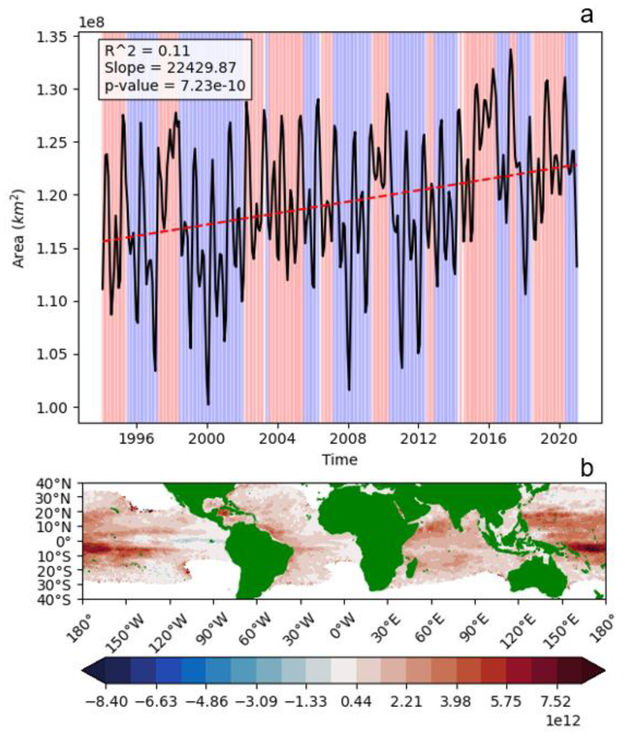
Figure 2.
Correlation with ENSO at lag = 0 of (a) OHC100, (b) OHCT, (c) ZAO, and (d) MAO. Linear annotations in (a) qualitatively delineate regions of alternating ENSO sign.
Figure 2.
Correlation with ENSO at lag = 0 of (a) OHC100, (b) OHCT, (c) ZAO, and (d) MAO. Linear annotations in (a) qualitatively delineate regions of alternating ENSO sign.
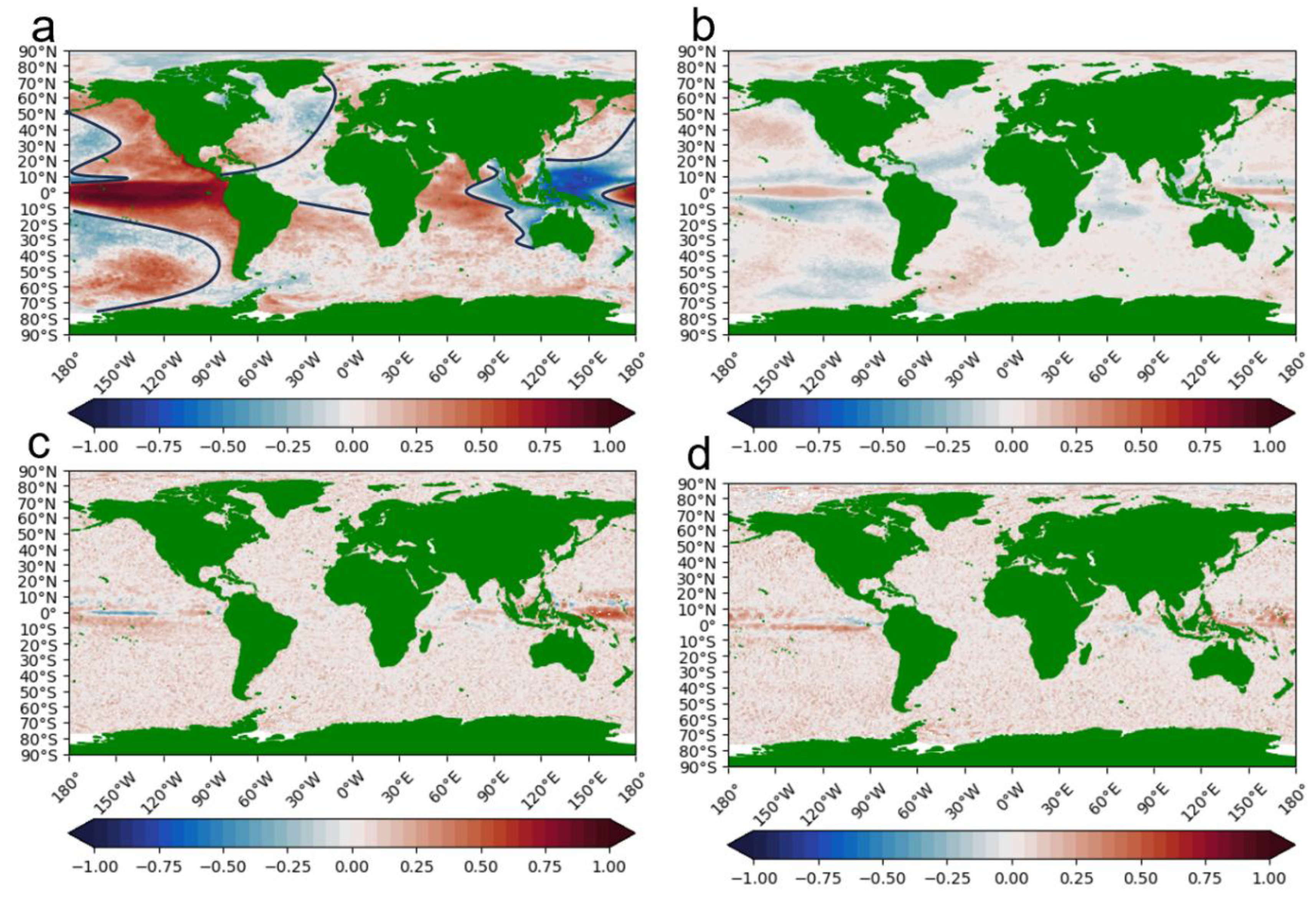
Figure 3.
Selected lag correlations between OHC100 and ENSO at ±12 month lags.
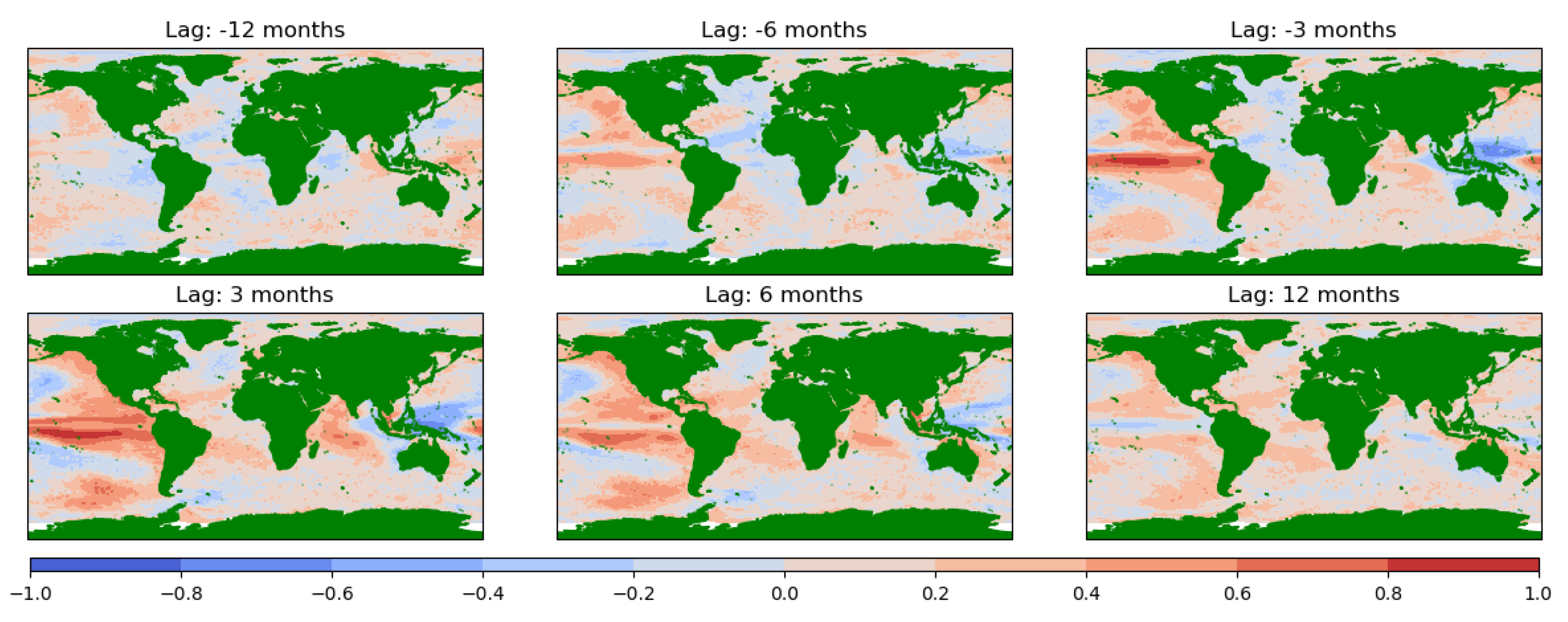
Figure 4.
Selected lag correlations between OHCT and ENSO at ±12 month lags.
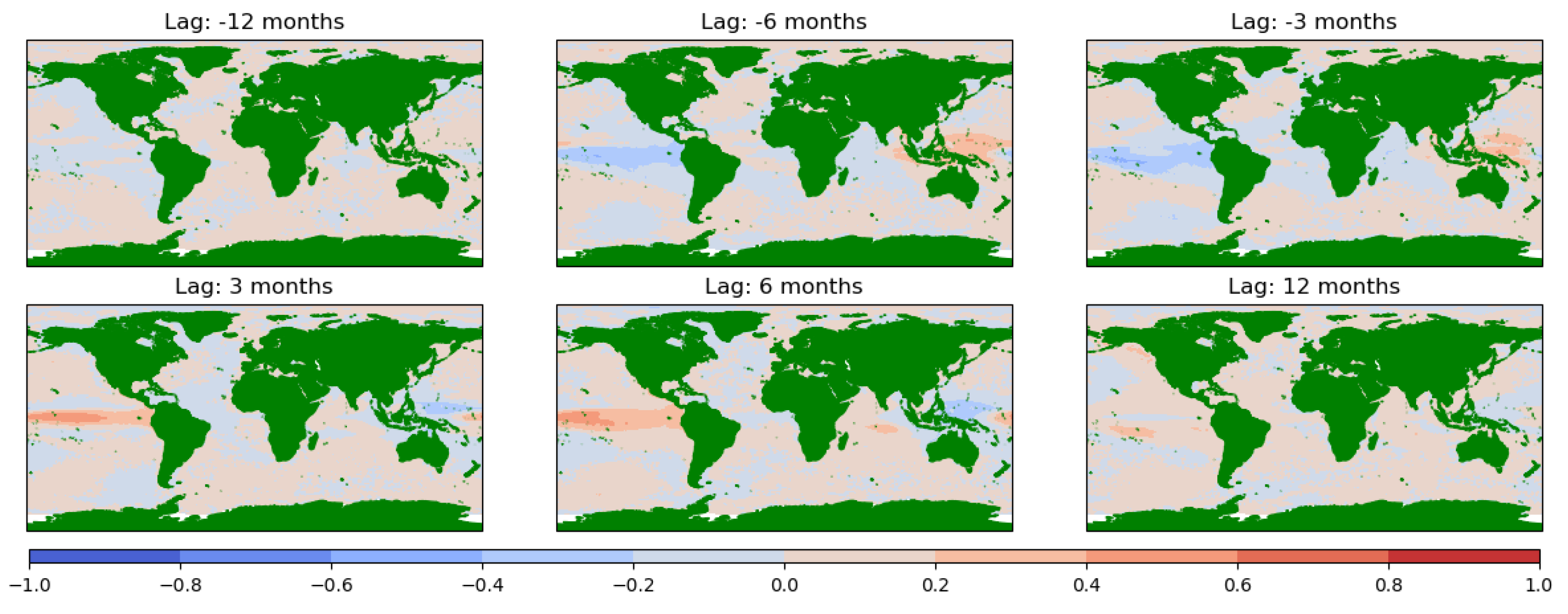
Figure 5.
Residuals of OHC100 (a); OHCT (b); ZAO (c); and MAO (d). The solid horizontal line marks the equator; dashed and dotted horizontal lines mark 10° and 30° north and south of the equator, respectively. Note the different units and scale of OHC100, a measure of heat, compared to the other three fluxes. Also note the factor of five difference between the larger ZAO and MAO scales and the OHCT scale.
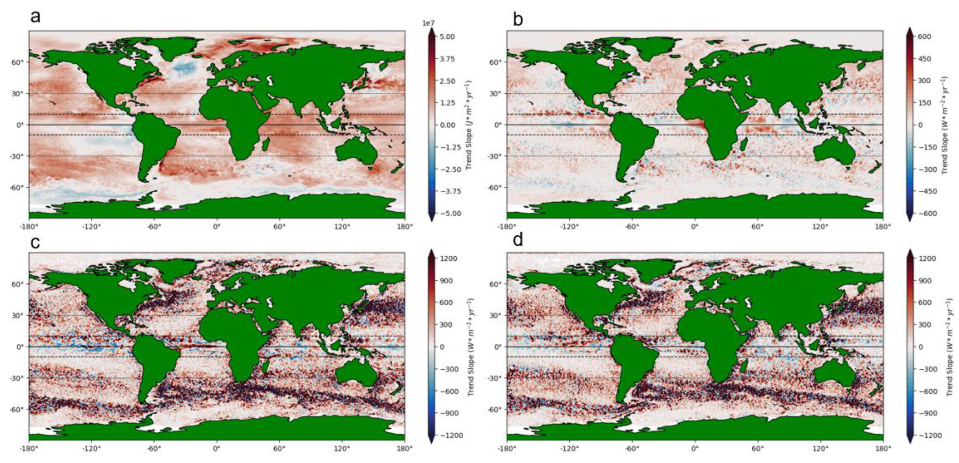
Disclaimer/Publisher’s Note: The statements, opinions and data contained in all publications are solely those of the individual author(s) and contributor(s) and not of MDPI and/or the editor(s). MDPI and/or the editor(s) disclaim responsibility for any injury to people or property resulting from any ideas, methods, instructions or products referred to in the content. |
© 2025 by the authors. Licensee MDPI, Basel, Switzerland. This article is an open access article distributed under the terms and conditions of the Creative Commons Attribution (CC BY) license (http://creativecommons.org/licenses/by/4.0/).
Copyright: This open access article is published under a Creative Commons CC BY 4.0 license, which permit the free download, distribution, and reuse, provided that the author and preprint are cited in any reuse.


