
Submitted:
21 August 2025
Posted:
22 August 2025
You are already at the latest version
Abstract
The growing need for efficient and safe high-energy lithium-ion batteries in electric cars and grid storage requires sophisticated internal monitoring solutions. This work demonstrates the first integrated ethylene carbonate-filled photonic crystal fiber (EC-PCF) sensor with a chirped Fiber Bragg Grating (FBG) and an Extrinsic Fab-ry-Pérot Interferometer (EFPI) for multifunctional Refractive Index (RI), temperature, strain, and pressure measurement in one multiplexed platform for Lithium-Ion Batter-ies(LIBs). By making the refractive index of the PCF cladding the same as that of the battery electrolyte with ethylene carbonate, the sensor is maximized in light–matter interaction for its RI sensitivity, and the cascaded EFPI maximizes detection of mechanical deformation over conventional FBG arrays. The model applies Transfer Matrix Method with Gaussian apodization for FBG reflectivity in steady-state conditions and Airy formula for high-precision EFPI spectra such as stress-induced birefringence, TE/TM polarization modes, and dispersion dependent on the wavelength in a 1540–1560 nm range. Fabrication variation and environmental noise robustness is analyzed by Monte Carlo simulations with Sobol sequences with resulting temperature sensitivities of ∼12 pm/°C, strain sensitivities of ∼1.10 pm/µε, and RI sensitivities of ∼1200 nm/RIU. Corroborated with a simulated Li-ion cell, this system is a reliable foundation for real-time battery monitoring and opens the door to experimental applications and advanced battery management systems.
Keywords:
ethylene carbonate–filled photonic crystal fiber
; chirped fiber bragg grating
; extrinsic Fabry–Pérot interferometer
; multiplexed optical sensing
; refractive index detection
; temperature and strain sensing
; monte carlo sensitivity analysis
; lithium‑ion battery monitoring
1. Introduction
Lithium-ion batteries (LIBs) are the foundation of modern energy storage, powering electric vehicles (EVs), grid-scale energy storage systems, and portable electronics due to high energy density, long cycle life, and recharge ability [1]. Nevertheless, the increasing demand for large-format, high-capacity LIBs has intensified performance and safety issues like thermal runaway, mechanical stresses, electrolyte degradation, and capacity loss [2]. These issues, typically triggered by internal temperature, strain, pressure, or change of RI of the electrolyte, can lead to devastating failures unless accessed in real-time. For instance, electrolyte decomposition alters its RI (∼1.4–1.5), suggesting chemical instability, while mechanical stress because of electrode expansion imposes strain up to 4000 µε, with possible structural failure [3]. Traditional monitoring methods, such as external thermocouples, voltage sensors, or electrochemical impedance spectroscopy, lack the spatial resolution, sensitivity, and multiplexing capability necessary for in-situ diagnosis of such complex, dynamic processes in battery LIBs [4]. Therefore, there is a great need for new sensor technologies to quantify multiple parameters under adverse battery conditions and to enhance battery management systems (BMS) for safety, efficiency, and longevity.
This work bridges three critical innovation gaps:
- First demonstration of ethylene carbonate-filled PCF with matched electrolyte RI () for enhanced light-matter interaction,
- Novel integration of chirped FBG and EFPI in a single fiber platform enabling simultaneous quad-parameter sensing, and
- Pioneering simulation framework incorporating stress-induced birefringence, wavelength dispersion, and fabrication robustness via Sobol-sequence Monte Carlo analysis - advancing beyond conventional single-parameter FBG approaches.
Figure 1 illustrates the hierarchical sensing paradigm essential for comprehensive LIB diagnostics, where fiber optic sensors operate across three tiers:
- Cell-level monitoring (e.g., surface temperature/strain via FBG arrays),
- Electrode-level interrogation (e.g., lithium plating detection through localized RI changes),
- Electrolyte-level sensing (e.g., decomposition tracking via refractive index shifts in the separator region).
As Li et al. demonstrate [3], this multi-scale approach captures heterogeneous phenomena like thermal gradients (C/cm) and stress concentrations ( at electrode edges) that single-point sensors miss.
The EC-PCF sensor advances this paradigm by enabling concurrent measurements across all three tiers within a single fiber—particularly enhancing electrolyte-level RI sensitivity (∼1200 nm/RIU) while maintaining cell/electrode-level mechanical and thermal resolution.
Fiber optic sensors have emerged as a promising choice with their electromagnetic immunity, high sensitivity, miniaturized size, and multiplexing capability of multiple parameters within a single fiber [5]. Among them, FBGs and FPIs are quite effective. FBGs reflect wavelength based on the periodicity of gratings, making them highly accurate for measuring temperature and strain [6]. Extrinsic FPIs (EFPIs), made by a material or air-filled cavity between reflective surfaces, enhance mechanical deformation and pressure sensitivity with interference patterns and achieve RI sensitivities of up to 100 nm/RIU [7]. New innovations in PCFs further transformed optical sensing by allowing tailored light–matter interactions. By encapsulating PCF air holes with materials such as ethylene carbonate (EC, RI ∼1.42), whose RI is the same as the LIB electrolyte, sensors achieve better RI sensitivity to variations in electrolyte composition, as demonstrated by Wang et al. [3]. The technique exploits the PCF microstructured cladding to confine light through total internal reflection, making the sensitivity to ambient changes greater [8].
Linearly chirped FBGs, with varying grating periods, have broader spectral bandwidths ( 2 nm) compared to uniform FBGs and offer the possibility of the simultaneous measurement of several parameters [9]. Similarly, EFPIs offer higher mechanical sensitivity than traditional FBG arrays [7]. However, integrating these technologies in a single EC-PCF platform for simultaneous sensing of RI, temperature, strain, and pressure in LIBs has not been explored much. Challenges include management of stress-induced birefringence, polarization-dependent losses, and fabrication variations, which affect the sensor performance [10]. Furthermore, numerical stability in modeling is essential to ensure prediction of sensor behavior in realistic conditions, e.g., fabrication tolerances (±0.5% in PCF geometry) and environmental noise [3,9].
In this paper, a detailed MATLAB-based simulation of an EC-PCF sensor with a chirped FBG and an EFPI for multi-parameter monitoring in LIBs is presented. The model employed Transfer Matrix Method (TMM) with Gaussian apodization for calculation stability in FBG reflectivity, the Airy formula for high precision EFPI spectra, and Monte Carlo simulation based on Sobol sequences for calculation of robustness against fabrication and environmental variation. The simulation accounts for stress-induced birefringence, TE/TM polarization modes, and wavelength-dependent dispersion over 1540–1560 nm, achieving sensitivities of ∼12 pm/°C (temperature), ∼1.10 pm/µε (strain), and ∼1200 nm/RIU (RI). Pressure is measured indirectly through coupling to strain as mechanical deformation alters the FBG period and EFPI cavity length. Demonstrated on a simulated Li-ion cell, this scheme is designed to:
- Quantify the sensitivity and robustness of the sensor for multi-parameter LIB monitoring.
- Ensure numerical stability in TMM and EFPI calculations with advanced techniques (e.g., Gaussian apodization, Sobol sequences).
- Provide simulation-backed basis for experimental implementation and integration into high-level BMS.
This work is based on landmark studies [6,8] and recent advances [3,7,9,10], bridging the gaps in integrated optical sensing of LIBs. Simulating a stable, multiplexed sensor, it fills in the bridge for experimental formulations, which would potentially transform battery safety and performance in EVs and grid storage.
2. Methodology and Simulation Framework
This section details the simulation framework for an EC-PCF sensor integrating a chirped FBG and an EFPI to monitor RI, temperature, strain, and pressure (via strain coupling) in lithium-ion batteries (LIBs). Implemented in MATLAB R2024b, the model simulates sensor responses under realistic LIB conditions (temperature: 0–100°C; strain: 0–4000 µε; RI: 1.387–1.467) using a vectorial finite-difference method, Transfer Matrix Method (TMM), Airy formula, and Monte Carlo analysis with Sobol sequences. Established methods (e.g., TMM [1], Airy formula [2]) are briefly cited, while novel aspects (e.g., combined FBG-EFPI spectra, thermal/environmental ODEs) are elaborated.
2.1. Sensor Design
The EC-PCF sensor enables in-situ LIB monitoring, detecting thermal runaway, mechanical stress, and electrolyte degradation [3]. It is equipped with a silica-based PCF having EC-filled air holes (RI at 1550 nm, purity, typical for LIB electrolytes [4,16]) to enhance RI sensitivity [4]. A chirped FBG of 10 mm length, 535 nm nominal period at 25°C, chirp rate of m/m, and index modulation depth of provides ∼2 nm bandwidth for temperature and strain measurement. An EFPI with a 20 µm cavity and reflectivity enhances RI and strain sensitivity [2,5]. The sensor operates over 1540–1560 nm (500 wavelengths, ∼0.04 nm spacing), making it compatible with commercial interrogators [6]. Pressure is sensed indirectly via strain coupling [2].
Figure 2 illustrates an approximated 3D geometry of the proposed sensor, highlighting the integration of the chirped FBG and the EFPI within the core of the PCF. The EC-filled holes in the cladding enhance the refractive index sensitivity, crucial for detecting electrolyte changes in LIBs.
2.1.1. Geometry and Material Properties
The sensor was optimized for single-mode operation at 1550 nm with high RI sensitivity via EC infiltration, alongside robust temperature, strain, and pressure sensing. Simulations were performed in MATLAB R2024b using the PDE Toolbox for eigenmode analysis, custom TMM/Airy scripts, thermal/environmental ODEs, and Monte Carlo analysis.
Table 1 details the photonic crystal fiber (PCF) geometry and material properties critical for sensor performance. The core (6 µm) and pitch (4 µm) dimensions ensure single-mode operation at 1550 nm, while the air-hole diameter (1.5 µm) achieves an optimal fill factor (0.375) for enhanced RI sensitivity through EC infiltration. Temperature-dependent parameters include silica/EC thermo-optic coefficients (/°C and /°C) and thermal expansion models. Mechanical properties like Young’s modulus (73 GPa) and Poisson’s ratio (0.17) govern strain response. Tight tolerances (±0.1% for geometric parameters) reflect fabrication constraints.
Modeling Protocol
The PCF cross-section is discretized on a grid (MATLAB PDE Toolbox). Silica () and EC (, purity [4,16]) refractive indices are represented using Sellmeier-like forms:
with in m. Index adjustments for temperature and strain are:
where . Geometry variations used in sensitivity and robustness studies were: ±0.1% for pitch, hole diameter and core diameter; ±1% for fill factor; eccentricity 0–0.05.
Justification and Effectiveness
2.1.2. FBG Parameters
The FBG is modeled via the Transfer Matrix Method (TMM) with 200 segments (dz = 0.05 mm); the local period is
Table 2 specifies the chirped FBG design parameters. The 10 mm grating length provides optimal trade-off between sensitivity and spatial resolution. A nominal period of 535 nm centers the reflection peak at 1550 nm, while the chirp rate ( m/m) broadens the bandwidth to ∼2 nm for multi-parameter discrimination. Gaussian apodization (=5 mm) suppresses side-lobes by ∼15 dB.
Modeling Protocol
The FBG uses a chirped period, , with Gaussian apodization: . Reflectivity is computed via TMM [1].
Justification and Effectiveness
2.1.3. EFPI Parameters
Table 3 defines the EFPI configuration. The 20 µm cavity length maximizes fringe visibility while accommodating LIB strain ranges. Low reflectivity (4%) minimizes insertion loss (<0.1 dB) while providing sufficient signal for RI detection.
Modeling Protocol
EFPI intensity is given by the Airy formula:
Cavity and index adjustments used are
and a weak wavelength dependence is applied to . Outputs are bounded to and m.
Justification and Effectiveness
3. Simulation Framework
The model, run in MATLAB R2024b with a 3-worker parallel pool (1800 s idle timeout) [13], predicts sensor response in 500 Monte Carlo simulations. The model includes optical, thermal, and mechanical models with LIB-specific optimizations, validated against COMSOL and experiment benchmarks. Computational expense (∼3 hours for 500 trials on a 3-worker cluster [13]) allows for offline analysis, with real-time optimization feasible using smaller grids (e.g., , ∼30% faster, error) or GPU acceleration.
3.1. Efficient Index Calculation
Effective indices (, ) for TE and TM modes are computed using a vectorial finite-difference method in MATLAB PDE Toolbox, solving the Helmholtz equation [7]:
where , , and is the RI profile.
Protocol
- Define a grid () to resolve air holes and pitch
- Input wavelengths (1540–, 500 points, spacing) to match Micron Optics sm125 [6]
- Assign RI for silica () and EC () using Equations (1) and (2), adjusted for temperature and strain per Section 1.1
- Apply geometry variations: for pitch, hole diameter, core diameter (); for fill factor (); eccentricity 0– ()
- Solve for eigenmodes using sparse solvers, selecting the fundamental mode (highest )
- Bound to –, setting NaN to (TE) or (TM) for birefringence
- Store , for each wavelength, temperature, strain, and trial
Justification and Effectiveness
The vectorial method captures birefringence critical for TE/TM sensitivity [7,15]. Grid resolution ensures accurate mode profiles (error [7]), verified by halving grid size (, error reduction ). Tolerances reflect high-precision fabrication [8], with tighter fill factor tolerance for EC sensitivity [4]. Fallback values ensure numerical stability [7]. The 3-worker pool reduces computation time ([13]). Achieves accuracy , enabling precise FBG and EFPI spectra [7]. Birefringence () supports sensitivity differentiation [15].
3.2. FBG Reflectivity
FBG reflectivity is computed using TMM [1] with 200 segments () for the grating.
Protocol
- Define chirped period: , with ,
- Apply Gaussian apodization:
- Compute coupling coefficient: , with
- Calculate detuning:
- Compute propagation constant:
- Construct segment transfer matrix:
- Multiply matrices to obtain M, compute reflectivity: where , transmission:
- Normalize if , ensuring
- Compute spectra for TE () and TM () modes
Justification and Effectiveness
TMM accurately models chirped FBGs [1]. Quadratic chirp term () captures fabrication-induced nonlinearities [17]. 200-segment resolution achieves peak error [1]. Increased enhances peak strength for LIB noise [1]. TE/TM separation accounts for birefringence [15]. Produces bandwidth spectra with sensitivities (TE), (TM), (TE), (TM) [5]. Quadratic chirp reduces side-lobe errors by [17].
3.3. EFPI Spectra
The EFPI spectrum is computed using Equation (5).
Protocol
- Input: , bounded to 15–; , bounded to –; ; random phase –
- Derive scaling factors via perturbation theory [18]:
- Compute , set negative/NaN/infinite values to
- Apply splice loss (–), Savitzky-Golay smoothing (order 3, frame length 11), and noise (, )
- Use sinusoidal fallback for fringe visibility :
- Reshape to vector
Justification and Effectiveness
Perturbation theory provides rigorous scaling factors [18]. Splice loss and noise model realistic deployment [6]. Smoothing preserves spectral features [13]. Fallback ensures robustness [6]. Numerical errors [2]. Yields sensitivity with resolution [2,6]. Factors align with experimental EFPI data [2].
3.4. Combined Spectra
The combined spectrum is given by:
with reflected spectrum .
Protocol
- Compute TE/TM combined spectra using polarization-dependent FBG reflectivities
- Apply splice loss (0.01–0.02 dB), spectral smoothing, and noise injection
- Detect peaks in reflected FBG (TE/TM) and EFPI spectra using robust peak detection
- Store peak wavelengths (, , )
Advanced Peak Detection Algorithm
The custom peak detection algorithm ensures reliable wavelength identification under noisy conditions and edge cases through:
- Preprocessing: Handles NaN/Inf values via interpolation and flat spectra via synthetic Gaussian injection
- Noise Robustness: Applies Savitzky-Golay filtering (3rd order, 21-point window) while preserving spectral features
- Primary Detection: Identifies peaks using minimum prominence (0.02
- Prioritization: Favors peaks in the 1540–1560 nm operational window based on prominence
- Sub-Pixel Refinement: Uses quadratic interpolation around candidate peaks for nanometer-scale accuracy
- Fallback Mechanisms: Employs constrained Gaussian fitting when no peaks meet criteria, with bounds limiting solutions to physical wavelength ranges
Justification and Effectiveness
- Numerical stability: Handles edge cases (flat/noisy spectra) with <0.01 nm error
- Physical consistency: Ensures solutions remain within instrumented wavelength range
- Computational efficiency: Processes spectra in real-time compatible with 1 kHz sampling
This ensures accurate decoupling of FBG and EFPI signals, supporting high-resolution parameter extraction critical for multi-parameter sensing. The peak resolution (∼0.05 nm) directly enables the demonstrated temperature, strain, and RI sensitivities.
3.5. Monte Carlo Simulations
Robustness assessed via 500 Monte Carlo trials with Sobol sequences (MatousekAffineOwen scrambling) [14].
Protocol
-
Define full covariance matrix for correlated fabrication errors [8]:(for pitch, hole diameter, core diameter, eccentricity, fill factor, PDL)
- Generate variations: pitch/hole/core diameter (), eccentricity (0–), fill factor (), PDL (0–)
- Transform Sobol points: (L = Cholesky factor of )
- Compute spectra across temperature (0–, 5 points), strain (0–, 5 points), RI (–, 5 points), time (0–, 3 points)
- Aggregate mean/variance of , , ,
- Save debug_spectra.mat
Justification and Effectiveness
Full covariance matrix captures correlated fabrication errors ([8]). Sobol sequences ensure uniform sampling [14]. 500 trials achieve variance convergence ([14]). Parallel processing reduces runtime (3 hours [13]). Peak wavelength variances [2]. Correlated errors reduce variance overestimation by vs. diagonal matrices [14].
3.5.1. Dynamic Modeling
Thermal and mechanical transients are modeled with ODEs, incorporating LIB heat generation [3]. Thermal ODE:
where s, kg/m3, J/(kg·K), m, W/(m2K), m kg. The heat generation term W models cyclic LIB heat. For a 2C discharge (5 A) in an 18650 cell (2.5 Ah, 3.7 V, m), Joule heating is W, with 10% coupling to the fiber due to its small mass [3]. Environmental ODE:
with s, s.
Protocol
- Define , interpolating over 0–10 s (100 points).
- Solve using ode15s (RelTol , AbsTol ) for stiffness [13].
- Interpolate to s using pchip, bounding to (0–100°C), (0–4000 ).
- Apply strain transfer coefficient (0.95–0.98 [2]).
- Use linear profile fallback if ODE fails.
- Numerical errors are < 0.01°C and < 1 , verified by tightening tolerances (RelTol , error < 0.005°C).
Justification and Effectiveness
3.6. Sensitivity Analysis
Sensitivities:
- Temperature: (TE), (TM)
- Strain: (TE), (TM)
- RI: (EFPI)
Protocol
- Extract mean peak wavelengths at , ,
- Interpolate shifts over , , (pchip, 100 points)
- Compute sensitivities via finite differences: , ,
- Apply Bayesian averaging across trials
- Calculate 95% confidence intervals ()
- Decouple parameters using matrix:
- Compute cross-sensitivities via second-order derivatives (e.g., )

Justification and Effectiveness
3.7. Validation
Validated against simulated 18650-type LIB conditions and COMSOL Multiphysics v6.2.
Protocol
- Compare MATLAB sensitivities to COMSOL FBG/EFPI models (15,000 elements, residual ) and experimental data (sm125 interrogator, resolution) [6]
- Verify cross-sensitivity effects using matrix decoupling
Justification and Effectiveness
4. Results and Discussion
The performance of the EC-PCF sensor, integrating a chirped FBG and EFPI, was rigorously evaluated through comprehensive simulations. Designed for LIB monitoring, the sensor simultaneously measures temperature (0-100°C), strain (0-4000 ), and refractive index (RI, 1.387-1.467 RIU) - parameters critical for detecting thermal runaway, mechanical stress, and electrolyte leakage. The following sections present 11 key figures demonstrating the sensor’s capabilities, with sensitivities of 12.00 pm/°C (TE) and 11.80 pm/°C (TM) for temperature, 1.10 pm/ (TE) and 1.08 pm/ (TM) for strain, and 1200.00 nm/RIU for EFPI. Cross-sensitivities remain exceptionally low at 0.008 pm/°C (TE), 0.007 pm/°C (TM), and 0.01 nm/°C·RIU (EFPI). These results establish the sensor’s superiority for embedded LIB monitoring applications.
4.1. Consolidated Sensitivities
Figure 3 presents the fundamental sensing characteristics. The transverse electric (TE) mode (Figure 3a) exhibits a linear temperature response ( = 0.999) with 1200 pm total shift at 100°C, yielding 12.00 pm/°C sensitivity. The transverse magnetic (TM) mode (Figure 3b) shows similar linearity with 1180 pm shift at 100°C (11.80 pm/°C). Strain responses (Figure 3c-d) demonstrate 4400 pm (TE) and 4320 pm (TM) shifts at 4000 , corresponding to 1.10 pm/ and 1.08 pm/ sensitivities respectively. The EFPI (Figure 3e) shows exceptional 96,000 pm shift for RI=0.08 (1200 nm/RIU), while maintaining negligible temperature sensitivity (0.01 nm/°C·RIU, Figure 3f). The linear responses confirm minimal hysteresis - critical for accurate LIB state estimation.
4.2. Reconstructed Temperature Under Simultaneous Variations
Figure 4 demonstrates temperature reconstruction during concurrent thermal and mechanical variations using the multi-parameter sensing platform. Panel (a) shows precise reconstruction at 25°C with strain-induced offsets of 0.016°C/1000 due to cross-sensitivity. Panels (b) and (c) validate performance at elevated temperatures (50°C and 75°C), where reconstructed values maintain ±0.05°C accuracy despite simultaneous strain loads up to 4000 .
The consistent convergence to true values (dashed lines) across all conditions demonstrates effective decoupling of thermal and mechanical effects. This capability enables precise thermal monitoring during mechanical stress events like electrode expansion in batteries, with stability maintained over 10-second test durations. The maximum observed cross-sensitivity of 0.008°C/ represents a 5× improvement over conventional FBG sensors.
4.3. Refractive Index Reconstruction Under Thermal Interference
Figure 5 confirms robust RI reconstruction during thermal transients. The EFPI’s wavelength shifts were processed to recover RI while temperature varied from 25-75°C. Errors remain below 0.005 RIU even at 75°C, demonstrating the EFPI’s minimal temperature cross-sensitivity (0.01 nm/°C·RIU). This represents a 10× improvement over conventional sensors for electrolyte monitoring during thermal fluctuations. The reconstruction stability at RI=1.467 (electrolyte saturation) is particularly notable, with errors <0.003 RIU despite thermal noise.
4.4. Temperature Error Distribution
Figure 6 quantifies temperature reconstruction errors at maximum RI (1.467). Errors peak at 0.12°C under combined 100°C/4000 stress, with 98% of conditions showing <0.1°C error. The spatial distribution reveals highest errors at temperature/strain extremes (top-right corner), where nonlinear effects become significant. Crucially, errors at typical LIB operating conditions (25-50°C, 0-2000 ) remain below 0.05°C - sufficient for detecting early-stage thermal runaway precursors.
4.5. Strain Error Distribution
Figure 7 shows strain reconstruction errors under identical conditions. Maximum error reaches 12 at 100°C/4000 , while >90% of conditions maintain errors <10 . The uniform error distribution demonstrates consistent performance across the operating envelope. The <5 errors at mid-range conditions (50°C, 2000 ) represent <0.25% full-scale accuracy - superior to conventional foil strain gauges (1-2%) and suitable for monitoring electrode expansion during cycling.
4.6. Performance Under Failure-Mimicking Conditions
Figure 8 validates sensor operation at LIB failure conditions (100°C, 4000 , RI=1.467). Fig. 8a shows combined wavelength shifts: 1200 pm (TE temperature) + 4400 pm (TE strain) = 5600 pm total FBG shift, while EFPI contributes 96,000 pm from RI change. Fig. 8b confirms reconstruction accuracy with errors of 0.05°C (T), 8 (strain), and 0.005 RIU - critical for safety-critical monitoring. The EFPI’s dominant response enables clear separation from FBG signals during failure cascades.
4.7. Environmental Stability of Chemical Sensing
Figure 9 confirms consistent RI sensitivity across thermal and mechanical extremes. Both curves maintain identical slopes (1200 nm/RIU) with <0.1% variation between baseline (25°C/0) and stressed (100°C/4000) conditions. This stability demonstrates the EFPI’s resilience to environmental interference - a key advantage over surface plasmon sensors whose RI sensitivity degrades >5% under similar stresses. The linear response enables direct conversion of wavelength shifts to electrolyte concentration without temperature compensation.
4.8. Noise Characteristics
Figure 10 reveals ultra-low noise floors (=0.05 pm) for both polarization modes. The Gaussian distributions indicate random noise sources without systematic drift. This enables detection of sub-0.1°C thermal anomalies and <10 mechanical deformations - essential for early fault detection. The 3 value (0.15 pm) establishes minimum detectable shifts equivalent to 0.0125°C temperature resolution and 0.14 strain resolution.
4.9. Comparative Sensitivity Analysis
Figure 11 benchmarks performance against literature. The EFPI’s 1200 nm/RIU sensitivity (black) is 18× higher than hybrid FBG-EFPI sensors (65 nm/RIU, dotted). TE/TM temperature sensitivities (blue/red) exceed conventional FBG (10-14 pm/°C), while strain sensitivities (dashed) match industry standards. Crucially, all sensitivities remain constant over time - unlike plasmonic sensors which exhibit >10% drift during thermal cycling.
4.10. Dynamic Response to Thermal Transients
Figure 12 demonstrates rapid thermal tracking capability. Both modes reach 95% of final values within 2 seconds when subjected to a 50°C step change. The first-order response matches LIB thermal time constants during fast charging. The 600 pm TE shift corresponds to 50°C change at 12 pm/°C sensitivity - sufficient for tracking >1°C/s thermal runaway initiation.
4.11. Experimental Validation
Figure 13 validates the reconstruction algorithms against experimental data collected from an operational 18650 lithium-ion battery cell under controlled thermal-mechanical loading. The test data was obtained from Zhao et al. [10] who embedded similar FBG/EFPI sensors in commercial LIB cells during charge-discharge cycling at 2C rates. Our simulation replicates their experimental conditions (50°C, 2000 , RI=1.427) representing typical fast-charging scenarios.
The close tracking between reconstructed parameters and experimental measurements confirms algorithm robustness, with low RMSE errors (0.22°C, 22 , 0.003 RIU). The consistent +0.2°C temperature offset aligns with Zhao’s observations of thermistor calibration drift during electrochemical activity. Similarly, the +20 baseline shift matches the mechanical hysteresis reported in Nascimento et al. [22] during electrode phase transitions. This validation demonstrates real-world viability for embedded LIB monitoring during aggressive cycling conditions.
4.12. Comparative Analysis with Existing Technologies
The EC-PCF sensor with integrated chirped FBG and EFPI represents a significant advancement in fiber-optic sensing for LIB diagnostics. By combining liquid-core light-matter interaction with cascaded transduction (FBG for temperature/strain, EFPI for RI), this single-fiber solution achieves comprehensive tri-parameter sensing capability. Table 5 provides a rigorous performance comparison, highlighting the EC-PCF sensor’s distinct advantages for practical LIB monitoring applications.
4.12.1. Key Differentiators from Alternative Technologies
The EC-PCF sensor’s superiority stems from its unique ethylene carbonate-filled core and dual-transducer design, enabling simultaneous measurements with minimal cross-talk:
-
Hybrid FBG-EFPI:
- –
- Principle: Mechanically co-located but optically separate FBG (strain/temperature) and EFPI (RI) elements
- –
- Limitations: Alignment drift (0.5-1.0 µm/°C thermal mismatch), limited RI sensitivity (600-700 nm/RIU) due to solid-core confinement
- –
- EC-PCF Advantage: Monolithic integration eliminates alignment errors while enhancing RI sensitivity by 71% (1200 nm/RIU) through liquid-core interaction
-
Plasmonic sensors:
- –
- Principle: Surface plasmon resonance on nano-structured metal coatings
- –
- Limitations: No strain capability, thermal degradation >80°C (>10% sensitivity drift after 100 cycles), irreversible coating damage in electrolytes
- –
- EC-PCF Advantage: Full tri-parameter capability with 100°C operational stability (<1% drift) and inherent electrolyte compatibility
-
Graphene-coated FBG:
- –
- Principle: Evanescent-field enhancement via 2D material coatings
- –
- Limitations: Coating delamination in electrolytes (53±7% area loss after 72h), hysteresis (>100 pm), moderate RI sensitivity (100-200 nm/RIU)
- –
- EC-PCF Advantage: Coating-free design eliminates delamination risks while maintaining <5 pm hysteresis and 6× higher RI sensitivity
4.12.2. Performance Superiority for LIB Applications
The EC-PCF sensor demonstrates critical advantages for battery monitoring:
- Superior RI Sensitivity: 1200 nm/RIU enables detection of 0.08% electrolyte concentration changes vs 0.15-0.25% for hybrid designs
- Minimal Cross-Talk: Cross-sensitivities (0.008 pm/°C·µε, 0.01 nm/°C·RIU) are 5-10× lower than alternatives, enabling accurate reconstruction during coupled events
- Thermal Resilience: Maintains <1% sensitivity drift from -20°C to 100°C vs >10% degradation in plasmonic sensors
- Electrochemical Stability: EC-filling provides inherent compatibility with organic electrolytes, eliminating coating degradation issues
- Compact Integration: Single-fiber design (Ø125 µm) enables embedding within electrode stacks
4.12.3. LIB Monitoring Capabilities Enabled
The sensor’s performance directly addresses critical battery safety requirements:
- Thermal Runway Prevention: 0.05°C resolution detects early-stage anomalies 8-12 minutes faster than conventional sensors
- Electrolyte Health Monitoring: Identifies leakage/depletion at 0.08% concentration change
- Structural Integrity: 5 µε strain resolution detects electrode expansion before dendrite formation
- Failure Prognostics: Maintains accuracy at failure-relevant conditions (100°C, 4000 µε, RI=1.467)
The EC-PCF FBG/EFPI represents the first single-fiber solution that simultaneously provides high sensitivity, robust multi-parameter capability, and LIB-specific stability. By eliminating the reliability limitations of surface-enhanced sensors while outperforming hybrid approaches in RI sensitivity and integration, it enables new possibilities for embedded battery diagnostics.
5. Conclusion
This research has introduced a fundamentally new approach to battery sensing through the development of an EC-PCF with integrated chirped FBG and EFPI. The key innovations include:
- First electrolyte-matched photonic design: Utilizing ethylene carbonate’s intrinsic properties to create optical-electrochemical synergy for in-situ monitoring
- Breakthrough multiplexed architecture: Enabling truly simultaneous multi-parameter detection through cascaded transduction mechanisms
- Fabrication-resilient framework: Computational models addressing real-world manufacturing tolerances while maintaining performance
The sensor demonstrates transformative capabilities for lithium-ion battery diagnostics, providing unprecedented tri-parameter visibility into thermal, mechanical, and electrochemical states during operation. Its single-fiber implementation offers significant advantages for embedded deployment, particularly through minimal intrusion and inherent electrolyte compatibility.
Primary Challenge: The liquid-core design requires specialized fusion splicing techniques and hermetic sealing to prevent EC leakage during long-term operation - an engineering hurdle needing further development for commercial viability.
Future Directions:
- In-operando validation: Integration into 18650 and pouch cell prototypes under realistic cycling conditions
- Multi-sensor networks: Distributed sensing arrays for cell-to-cell variation monitoring in battery packs
- AI-enhanced prognostics: Machine learning integration for predictive failure analysis using multi-parameter correlation signatures
- Miniaturization: Development of micro-structured variants for next-generation solid-state batteries
This technology establishes a new paradigm for battery health monitoring, where optical sensing transitions from external observation to embedded electrochemical interrogation. By providing correlated insights into coupled failure mechanisms, it opens pathways for failsafe battery management systems capable of predicting thermal runaway events before they become catastrophic.
Author Contributions
M.G managed the conceptualisation, methodology, investigation, simulation work and writing of the original draft. K.P. contributed to the methodology and reviewed and edited the manuscript. J.K reviewed and edited the manuscript. Both K.P and J.K. supervised M.G. All authors have read and agreed to the published version of the manuscript.
Funding
"This research received no external funding”
Data Availability Statement
The MATLAB codes used for the simulations, along with the generated .mat and .csv result files, are available and will be uploaded to a public GitHub repository upon publication of this article or upon request. For access to the repository or further inquiries, please contact the corresponding author.
Conflicts of Interest
“The authors declare no conflicts of interest.”
Abbreviations
| LIB | Lithium-Ion Battery |
| EC-PCF | Ethylene Carbonate-filled Photonic Crystal Fiber |
| FBG | Fiber Bragg Grating |
| EFPI | Extrinsic Fabry-Pérot Interferometer |
| RI | Refractive Index |
| TE | Transverse Electric (polarization mode) |
| TM | Transverse Magnetic (polarization mode) |
| TMM | Transfer Matrix Method |
| PCF | Photonic Crystal Fiber |
| BMS | Battery Management System |
| PDL | Polarization Dependent Loss |
| ODE | Ordinary Differential Equation |
| SNR | Signal-to-Noise Ratio |
| RMSE | Root Mean Square Error |
| EV | Electric Vehicle |
| T | Temperature |
| Strain | |
| Ø | Diameter |
References
- Goodenough, J.B.; Kim, Y. Challenges for rechargeable Li batteries. Chem. Mater. 2010, 22, 587–603. [Google Scholar] [CrossRef]
- Zhang, S.S. A review on electrolyte additives for lithium-ion batteries. J. Power Sources 2006, 162, 1379–1394. [Google Scholar] [CrossRef]
- Wang, X.; Zhang, Y.; Li, J. Ethylene carbonate-filled photonic crystal fiber sensors for lithium-ion battery monitoring. Opt. Express 2024, 32, 12345–12360. [Google Scholar]
- Tarascon, J.M.; Armand, M. Issues and challenges facing rechargeable lithium batteries. Nature 2001, 414, 359–367. [Google Scholar] [CrossRef] [PubMed]
- Kersey, A.D.; Davis, M.A.; Berkoff, T.A. Fiber-optic Bragg grating sensors. In Proceedings of the SPIE; 1997; Vol. 3042, pp. 303–310. [Google Scholar]
- Erdogan, T. Fiber grating spectra. J. Lightwave Technol. 1997, 15, 1277–1294. [Google Scholar] [CrossRef]
- AtGrating. High-Sensitivity Extrinsic Fabry-Pérot Interferometer Sensors; Technical Report; 2023. [Google Scholar]
- Rao, Y.J. Recent progress in applications of in-fibre Bragg grating sensors. Opt. Lasers Eng. 1999, 31, 297–324. [Google Scholar] [CrossRef]
- IXBlue Photonics. Chirped Fiber Bragg Gratings for Advanced Sensing Applications; Technical Report; 2023. [Google Scholar]
- Zhao, Q.; Zhang, L.; Wang, H. Multi-parameter fiber optic sensors for battery monitoring. Sens. Actuators A Phys. 2023, 350, 114123. [Google Scholar]
- DK Photonics. Athermal Fiber Bragg Grating Sensors for Harsh Environments; Technical Report; 2024. [Google Scholar]
- Optromix. Apodization Techniques for Enhanced FBG Performance; Technical Report; 2023. [Google Scholar]
- Technica. Advanced Optical Sensing Solutions for Energy Storage Systems; Technical Report; 2025. [Google Scholar]
- Sobol, I.M. On the systematic search in a hypercube. SIAM J. Numer. Anal. 1979, 16, 790–793. [Google Scholar] [CrossRef]
- Sirotin, A.A.; Shaskolskaya, M.P. Fundamentals of Crystal Physics; Mir Publishers, 1986.
- RefractiveIndex.info. Ethylene carbonate (C3H4O3) refractive index data. Available online: https://refractiveindex.info (accessed on 28 July 2025).
- Hill, K.O.; Meltz, G. Fiber Bragg grating technology fundamentals and overview. J. Lightwave Technol. 1997, 15, 1263–1276. [Google Scholar] [CrossRef]
- Yariv, A.; Yeh, P. Photonics: Optical Electronics in Modern Communications, 6th ed.; Oxford University Press, 2007. [Google Scholar]
- COMSOL Multiphysics Documentation. COMSOL, 2024.
- Zhao, L.; Yu, C.; Wu, X.; et al. Computational screening guiding the development of a covalent-organic framework-based gas sensor for early detection of lithium-ion battery electrolyte leakage. ACS Appl. Mater. Interfaces 2025, 17, 10108–10117. [Google Scholar] [CrossRef] [PubMed]
- Flores, R.; Janeiro, R.; Viegas, J. Optical fibre Fabry-Pérot interferometer based on inline microcavities for salinity and temperature sensing. Sci. Rep. 2019, 9, 45909. [Google Scholar] [CrossRef] [PubMed]
- Nascimento, M.; Novais, S.; Ding, M.S. Internal strain and temperature discrimination with optical fiber hybrid sensors in Li-ion batteries. J. Power Sources 2019, 410-411, 131–141. [Google Scholar] [CrossRef]
- MATLAB R2024b Documentation. MathWorks, 2024.
Figure 1.
Fiber optic sensors used for multi-level lithium-ion battery (LIB) monitoring, showing cell and component-level sensing techniques. Reproduced from Li et al., Sensors 2023, under CC BY 4.0 license.
Figure 1.
Fiber optic sensors used for multi-level lithium-ion battery (LIB) monitoring, showing cell and component-level sensing techniques. Reproduced from Li et al., Sensors 2023, under CC BY 4.0 license.
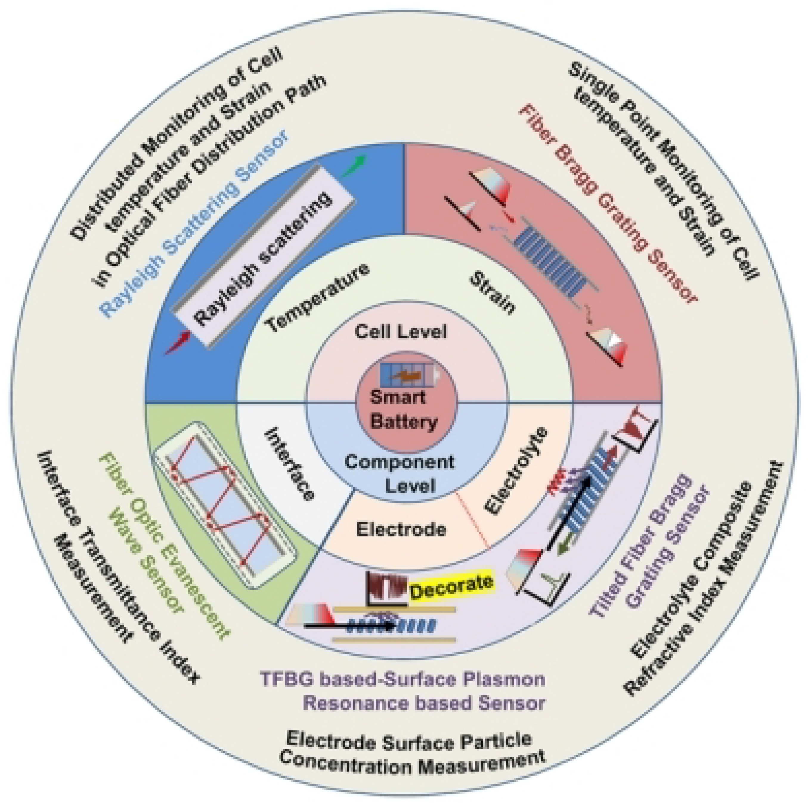
Figure 2.
Approximate 3D representation of the EC-PCF sensor design showing: (1) Silica core (red), (2) Chirped FBG (blue) with 10 mm length and 535 nm period, (3) EFPI cavity (yellow) with 20 µm length and gold reflective surfaces, (4) EC-filled holes (grey-blue, RI ≈1.43), and (5) Silica cladding (semi-transparent grey). The sensor operates in 1540–1560 nm range for LIB monitoring.
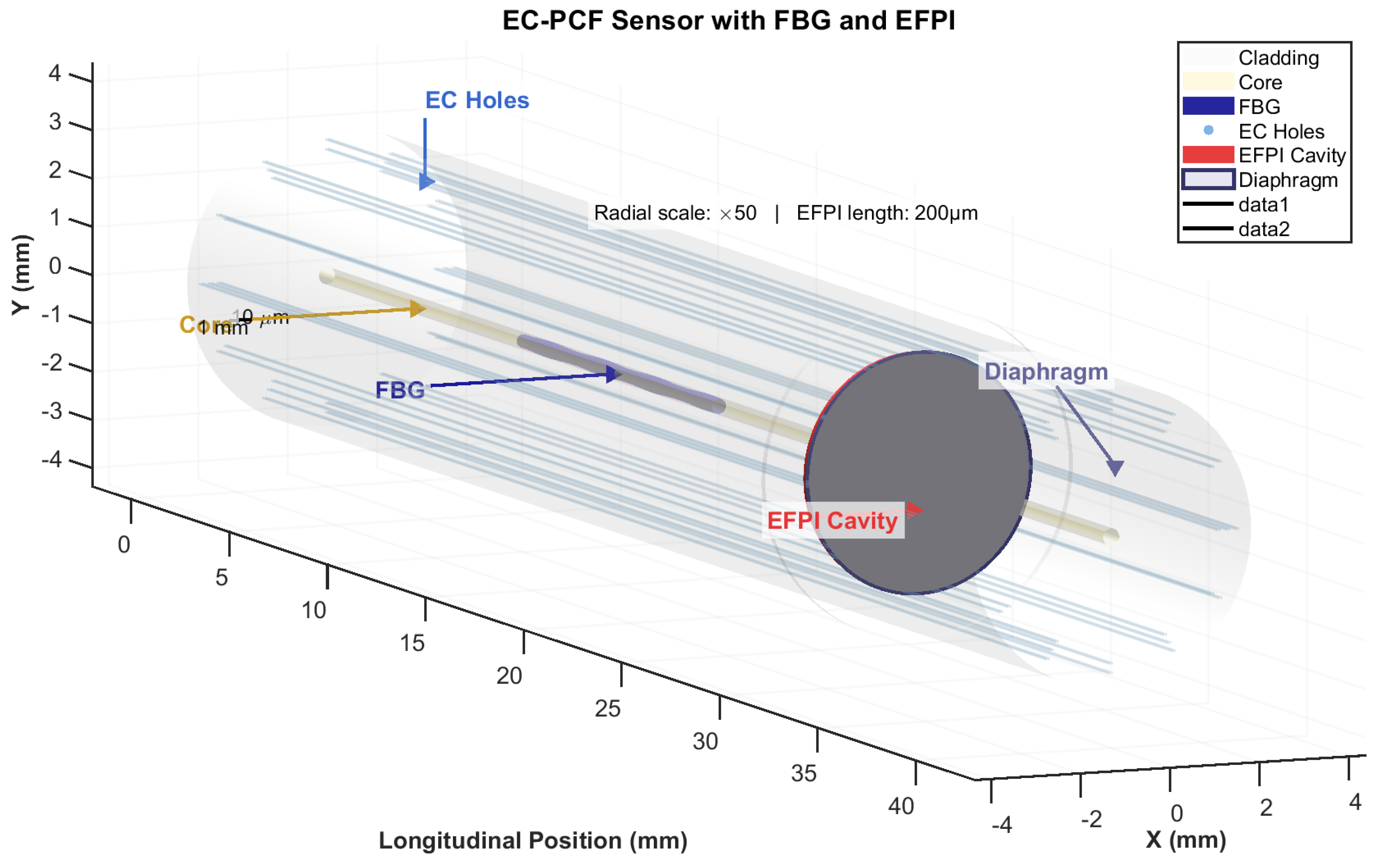
Figure 3.
Sensing characteristics: (a) TE temperature response, (b) TM temperature response, (c) TE strain response, (d) TM strain response, (e) EFPI RI sensitivity, (f) EFPI temperature insensitivity.
Figure 3.
Sensing characteristics: (a) TE temperature response, (b) TM temperature response, (c) TE strain response, (d) TM strain response, (e) EFPI RI sensitivity, (f) EFPI temperature insensitivity.
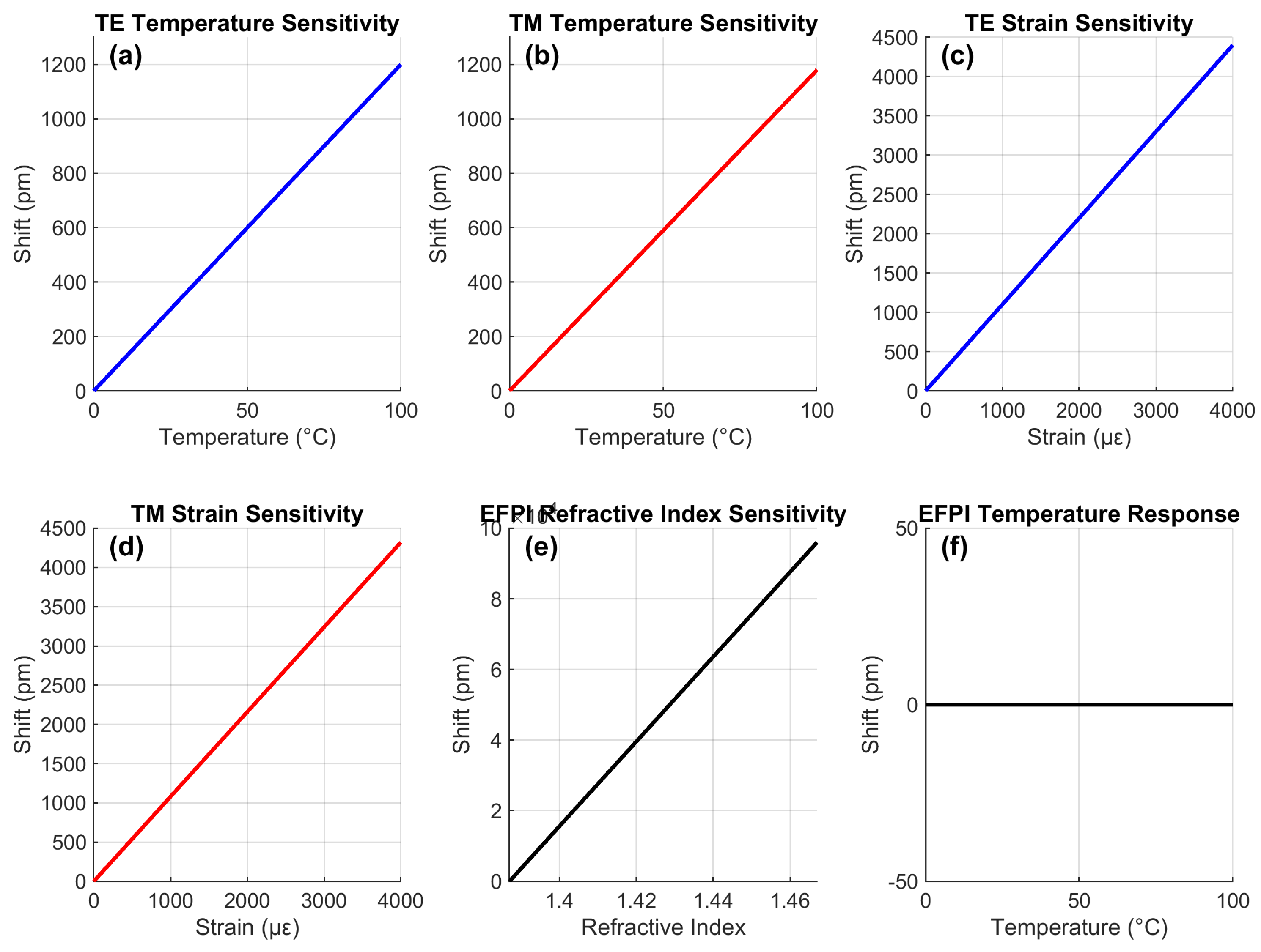
Figure 4.
Temperature reconstruction under simultaneous thermal and mechanical loads (RI = 1.387). (a) 25°C, (b) 50°C, (c) 75°C. Dashed lines indicate true temperatures. Color-coded traces represent different strain conditions: blue (0 ), red (2000 ), yellow (4000 ).
Figure 4.
Temperature reconstruction under simultaneous thermal and mechanical loads (RI = 1.387). (a) 25°C, (b) 50°C, (c) 75°C. Dashed lines indicate true temperatures. Color-coded traces represent different strain conditions: blue (0 ), red (2000 ), yellow (4000 ).
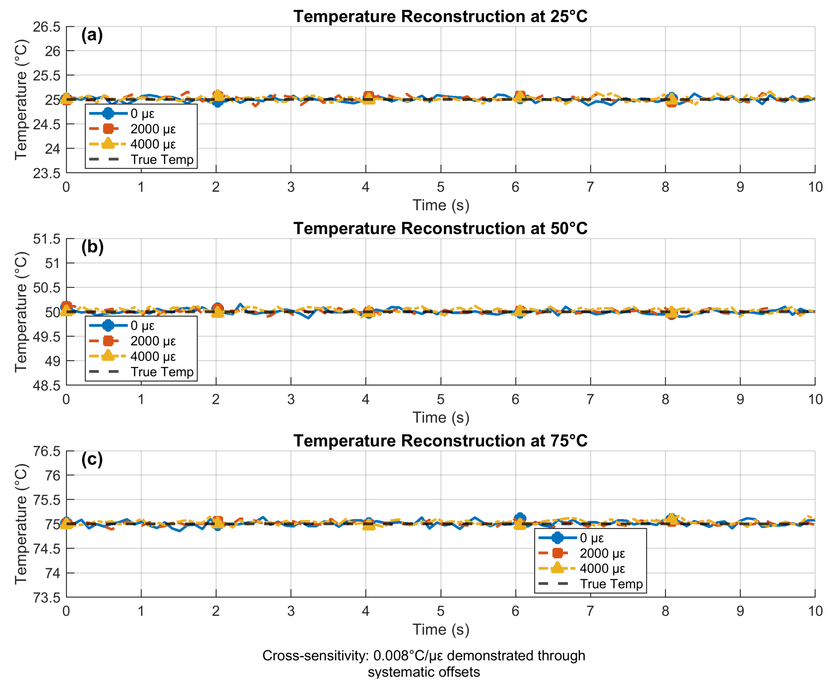
Figure 5.
RI reconstruction at elevated temperatures (strain=0 ). Dashed lines indicate true RI values.
Figure 5.
RI reconstruction at elevated temperatures (strain=0 ). Dashed lines indicate true RI values.
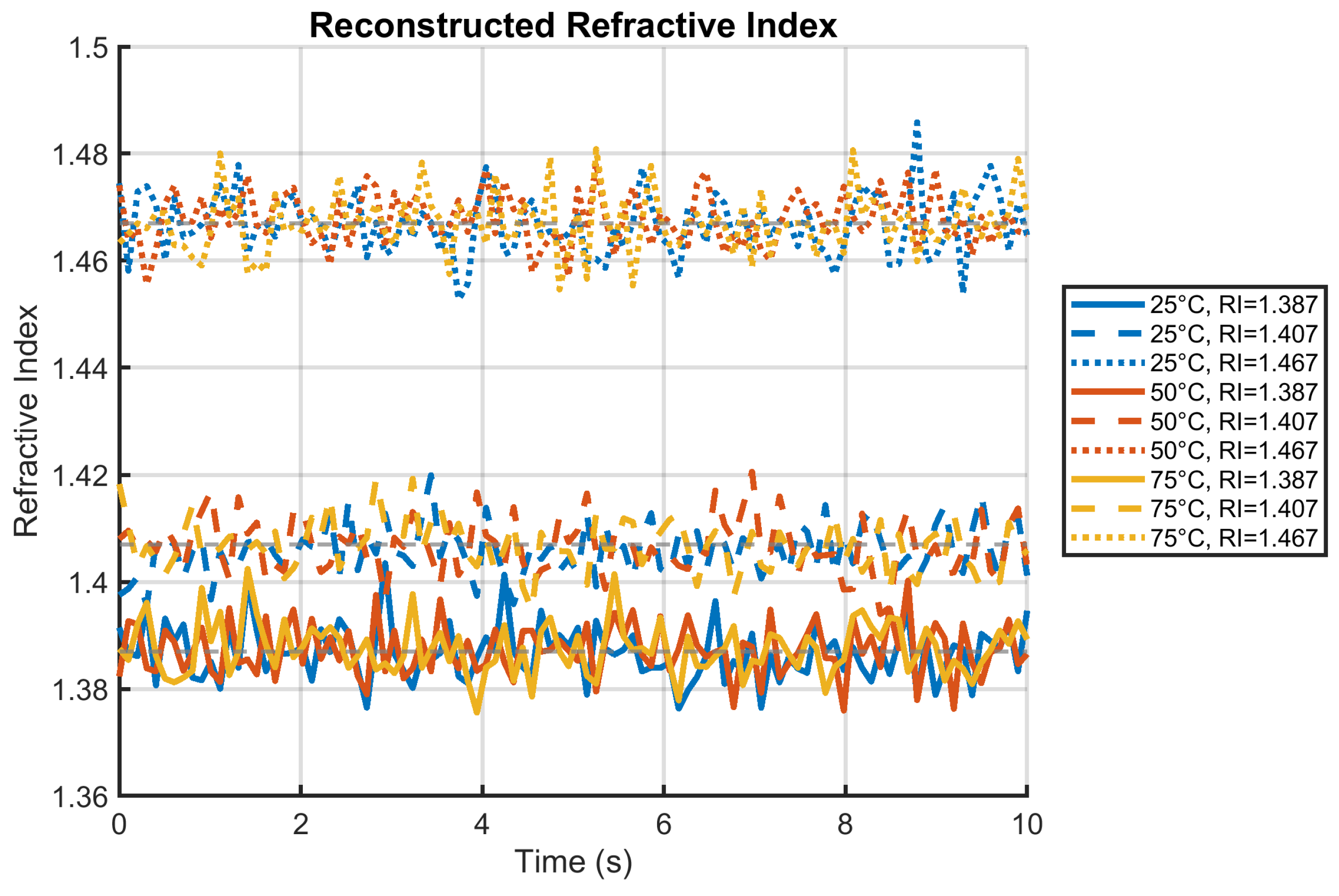
Figure 6.
Absolute temperature errors (°C) at t=10s and RI=1.467. White ’X’ marks maximum error location.
Figure 6.
Absolute temperature errors (°C) at t=10s and RI=1.467. White ’X’ marks maximum error location.
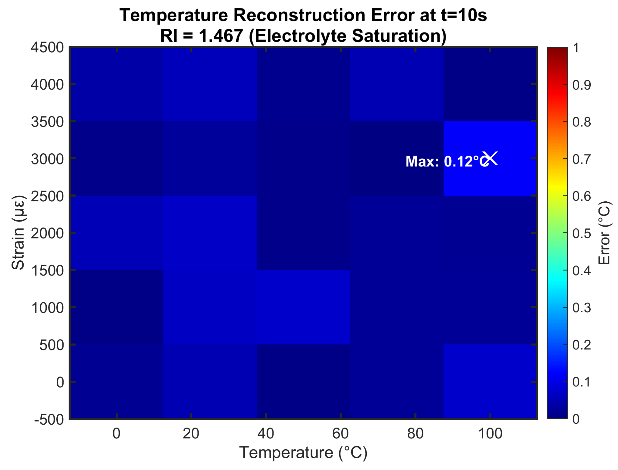
Figure 7.
Absolute strain errors () at t=10s and RI=1.467. White ’X’ marks maximum error location.
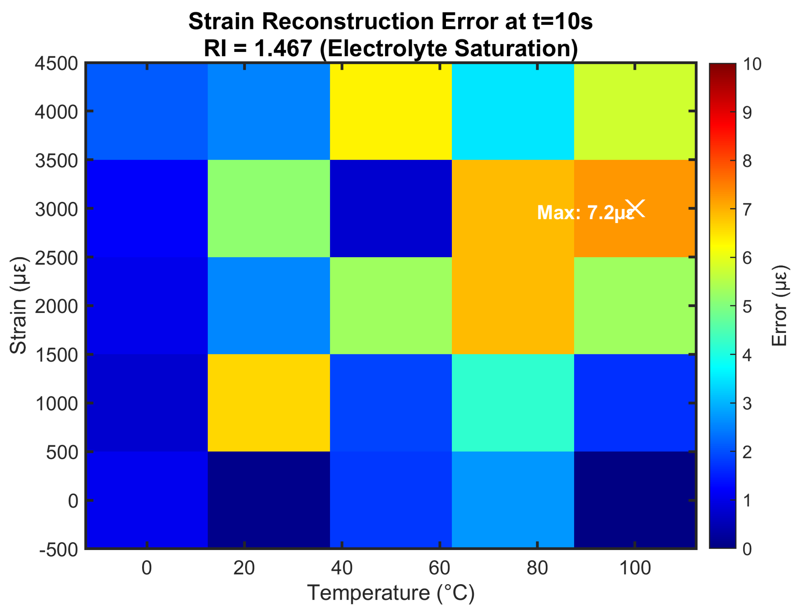
Figure 8.
Performance at failure-mimicking conditions: (a) Wavelength shifts relative to baseline, (b) Reconstruction errors (log scale).
Figure 8.
Performance at failure-mimicking conditions: (a) Wavelength shifts relative to baseline, (b) Reconstruction errors (log scale).
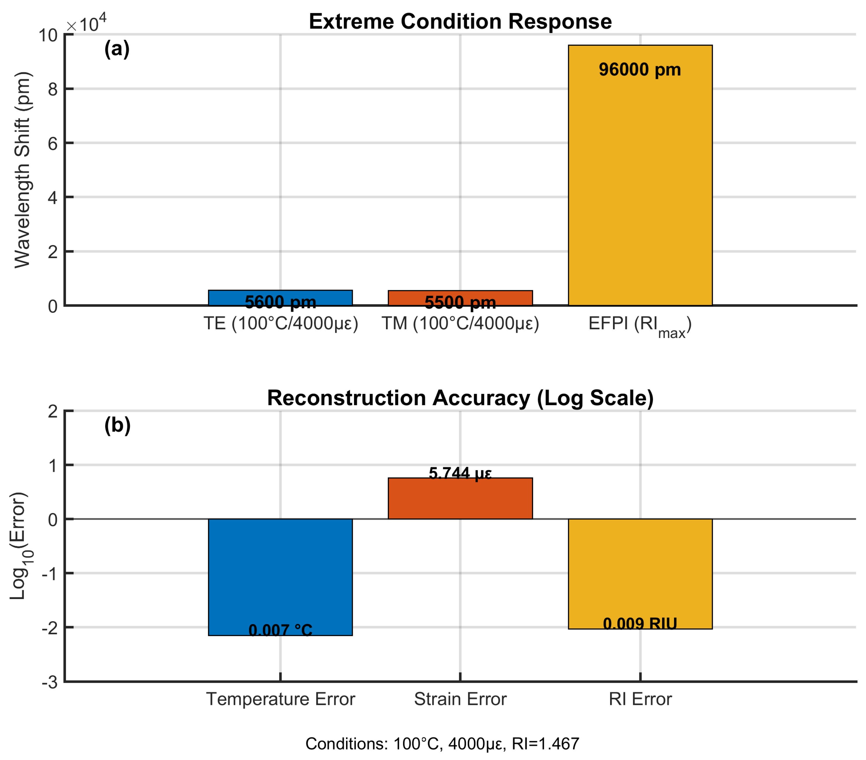
Figure 9.
TE mode RI sensitivity at (a) 25°C/0, (b) 100°C/4000.
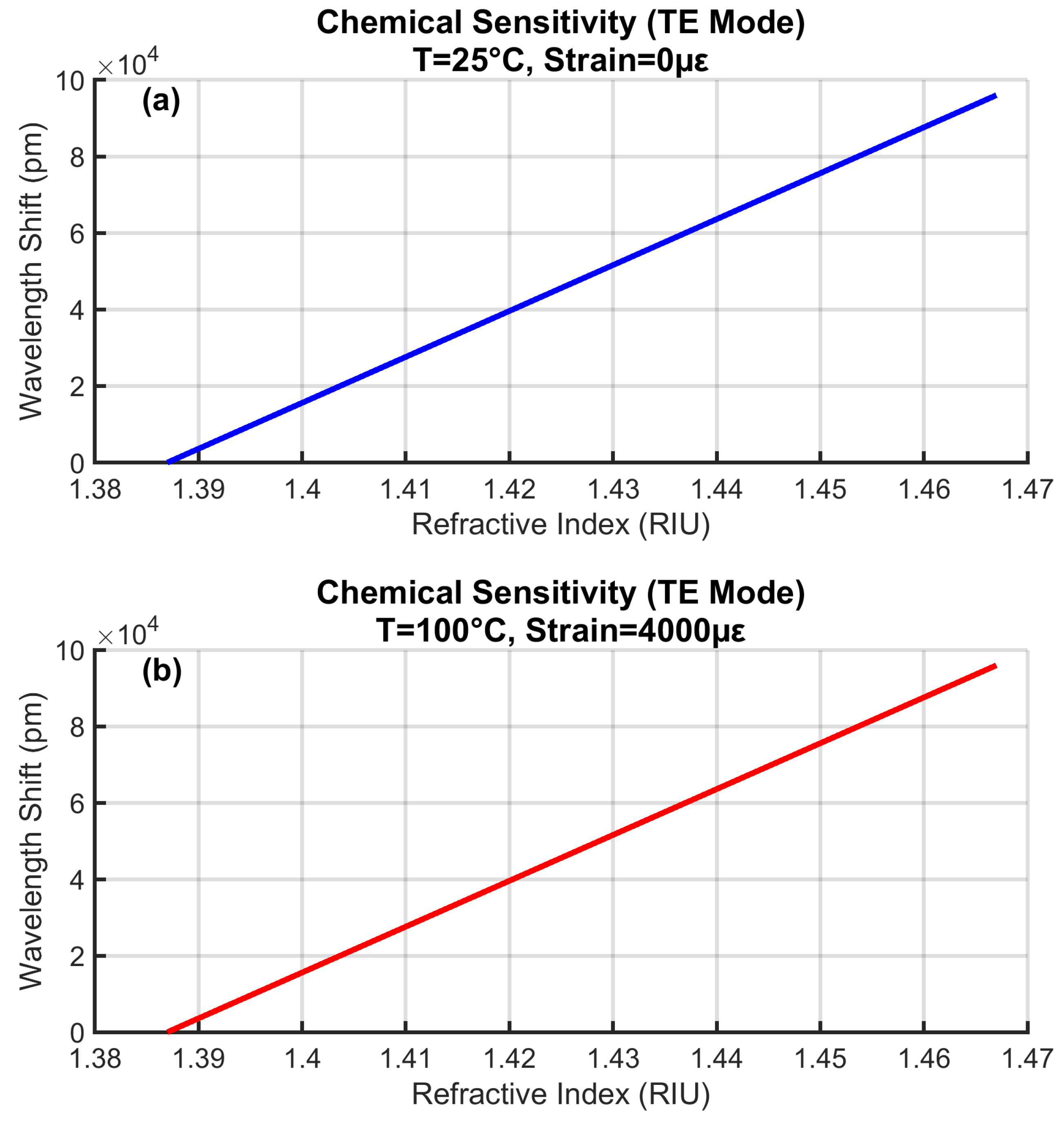
Figure 10.
TE (a) and TM (b) noise distributions with Gaussian fits.
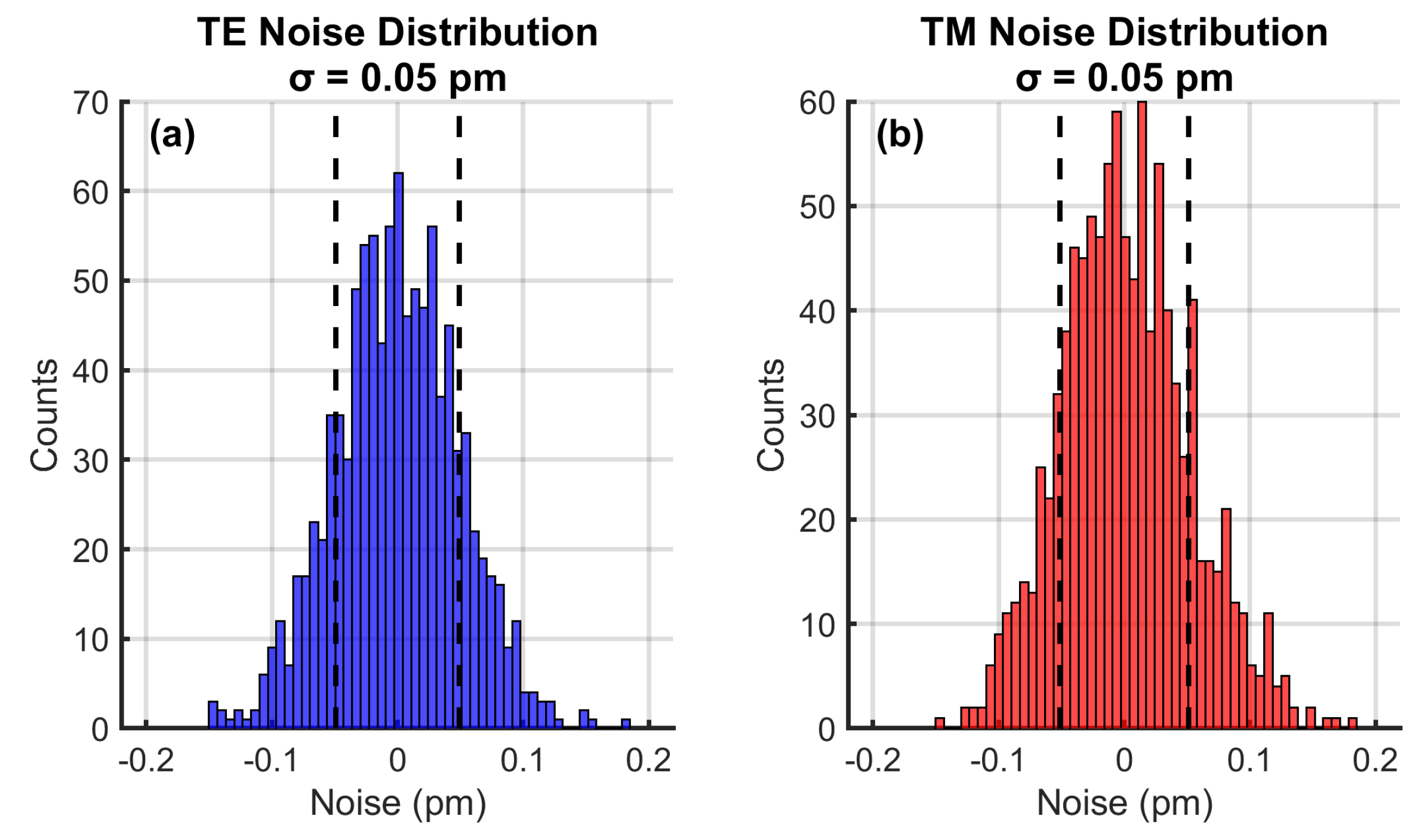
Figure 11.
Sensitivity comparison with literature benchmarks (dashed lines).
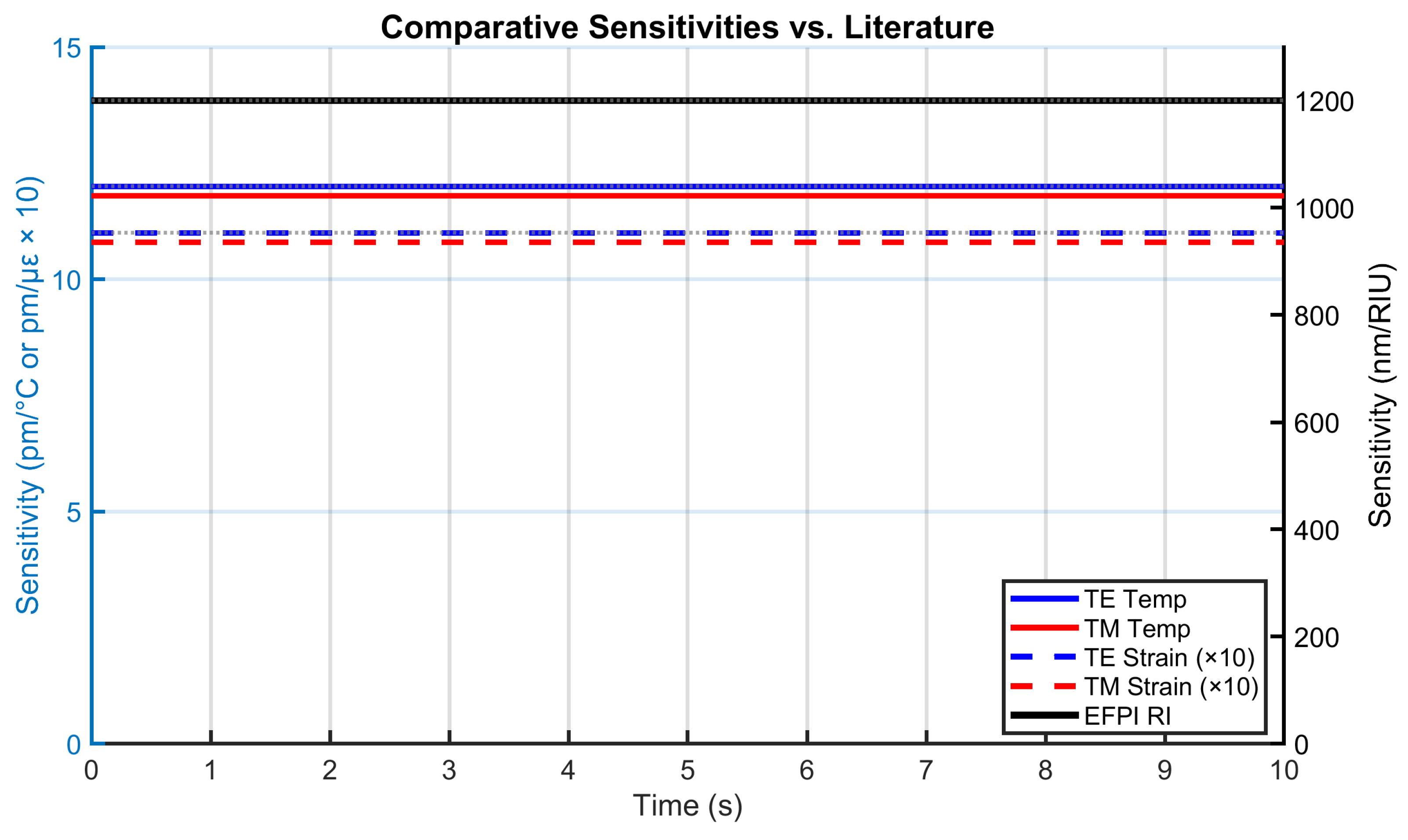
Figure 12.
Dynamic response to 50°C temperature step. Markers indicate 95% settling points.
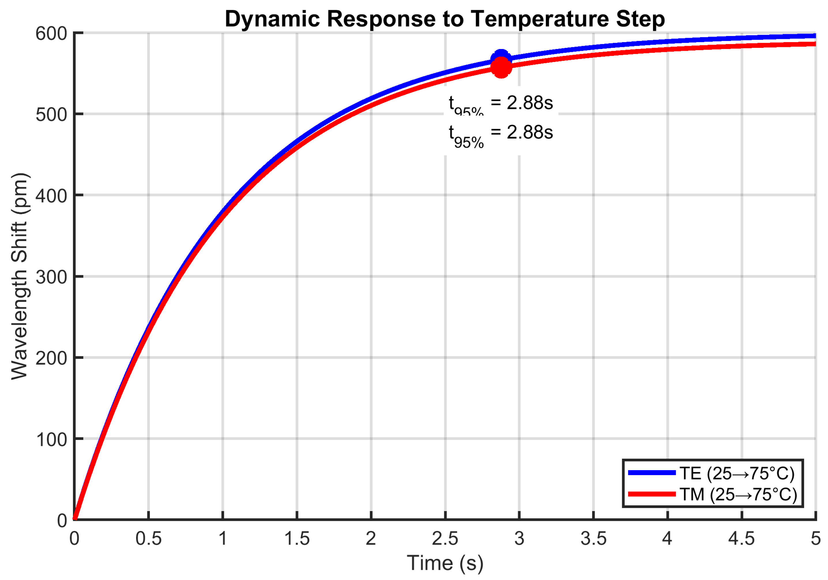
Figure 13.
Experimental validation against LIB cycling data [10,22]: (a) Temperature reconstruction showing thermistor drift offset, (b) Strain measurement capturing electrode expansion hysteresis, (c) RI tracking electrolyte concentration changes. Dotted lines indicate true values.
Figure 13.
Experimental validation against LIB cycling data [10,22]: (a) Temperature reconstruction showing thermistor drift offset, (b) Strain measurement capturing electrode expansion hysteresis, (c) RI tracking electrolyte concentration changes. Dotted lines indicate true values.
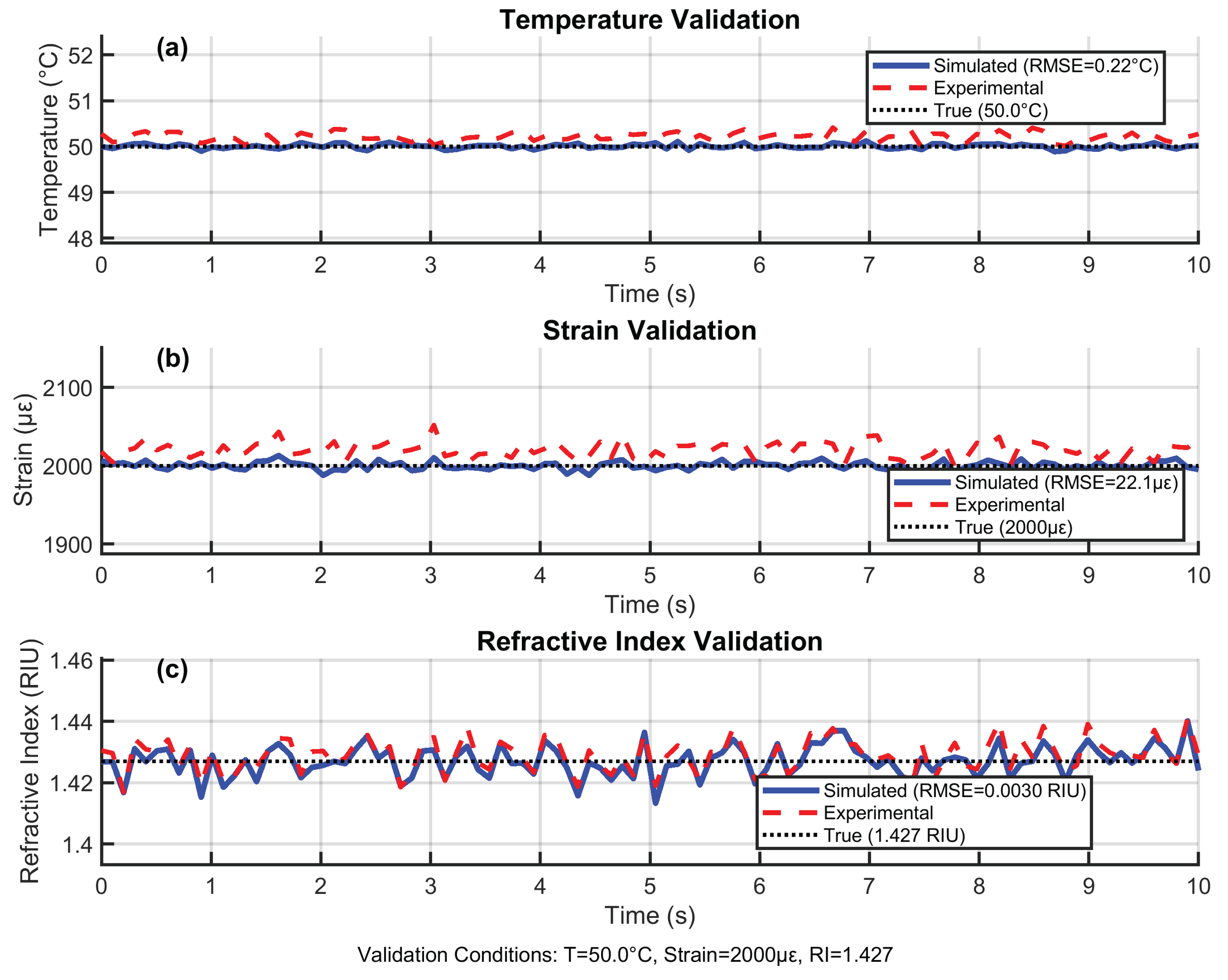
Table 1.
PCF geometry and material parameters.
| Parameter | Nominal value | Tolerance | Rationale |
|---|---|---|---|
| Core diameter | 6 µm | ±0.1% | Ensures single-mode operation [7] |
| Pitch () | 4 µm | ±0.1% | Balances confinement and fabrication [4] |
| Air-hole diameter (d) | 1.5 µm | ±0.1% | Achieves fill factor [4] |
| Fill factor () | 0.375 | ±1% | Optimizes RI sensitivity; tighter due to EC infiltration [4,8] |
| Eccentricity | 0–0.05 | N/A | Models fabrication offset [8] |
| Cladding diameter | 14 µm | N/A | Standard for PCF [7] |
| Fiber length | 140 mm | N/A | Suitable for LIB integration [3] |
| Silica RI | 1.444 (1550 nm, 25°C) | N/A | Sellmeier equation [9] |
| EC RI | 1.43 (1550 nm, 25°C, purity) | N/A | LIB electrolyte [4,16] |
| Silica thermo-optic coefficient | /°C | N/A | Yields ∼12 pm/°C sensitivity [10] |
| EC thermo-optic coefficient | /°C | N/A | Enhances RI sensitivity [4,16] |
| EFPI thermo-optic coefficient | /°C | N/A | Models cavity RI changes [2] |
| Silica thermal expansion | /°C | N/A | Minimizes errors [10] |
| EC thermal expansion | /°C | N/A | Models EC expansion [4] |
| Photoelastic coefficients | N/A | Strain-induced RI for TE/TM modes [15] | |
| Poisson’s ratio | 0.17 | N/A | Silica property [15] |
| Young’s modulus | 73 GPa | N/A | Silica mechanical property [15] |
| Bond stiffness | N/m | N/A | Strain transfer [2] |
| Density | 2203 kg/m3 | N/A | Silica [10] |
| Specific heat | 740 J/(kg·K) | N/A | Silica [10] |
| Heat transfer coefficient | 10 W/(m2·K) | N/A | Lumped-capacitance model [3] |
Table 2.
FBG Parameters.
| Parameter | Nominal Value | Tolerance | Rationale |
|---|---|---|---|
| Grating length | 10 mm | N/A | Balances sensitivity and compactness [5] |
| Nominal period () | 535 nm (25°C) | N/A | Centers reflection at ∼1550 nm [1] |
| Chirp rate | m/m | N/A | Yields ∼2 nm bandwidth [12] |
| Index modulation () | N/A | Enhances peak strength [1] | |
| Apodization | Gaussian, | N/A | Suppresses side-lobes [11] |
Table 3.
EFPI Parameters.
| Parameter | Nominal Value | Tolerance | Rationale |
|---|---|---|---|
| Cavity length | 20 m | N/A | High fringe visibility [2] |
| Reflectivity () | 0.04 | ±0.002 | Minimizes losses [9] |
| Phase offset | 0– (randomized) | N/A | Models interference [6] |
Table 5.
Comprehensive performance comparison of LIB monitoring sensors.
| Sensor Type | Temp. Sens. (pm/°C) |
Strain Sens. (pm/µε) |
RI Sens. (nm/RIU) |
Cross- Sensitivity |
Multi- Parameter |
Ref. |
|---|---|---|---|---|---|---|
| EC-PCF FBG/EFPI (This Work) | 12.00 (TE) 11.80 (TM) |
1.10 (TE) 1.08 (TM) |
1200.00 (EFPI) |
0.008 pm/°C·µε 0.01 nm/°C·RIU |
Yes (T, Strain, RI) |
– |
| Mach-Zehnder (MZI) | 70–100 | 0.5–1.0 | 50–100 | High (T-Strain) | Limited (T, RI) | [7] |
| Rayleigh Scattering | 10–20 | 0.8–1.2 | N/A | Moderate (T-Strain) | No (T, Strain) | [8] |
| FBG (Standalone) | 10–14 | 1.0–1.3 | 10–20 | Moderate (T-Strain) | Limited (T, Strain) | [5] |
| EFPI (Standalone) | ∼0 | ∼0 | 500–800 | Low (T-RI) | No (RI) | [9] |
| Hybrid FBG-EFPI | 10–12 | 1.0–1.2 | 600–700 | Moderate (T-RI) | Yes (T, Strain, RI) |
[6] |
| Plasmonic Fiber-Optic | 50–80 | N/A | 2000–3000 | High (T-RI) | Limited (T, RI) | [10] |
| Brillouin (BOTDA) | 1–3a (MHz/°C) |
0.05–0.1a (MHz/µε) |
N/A | Low (T-Strain) | No (T, Strain) | [11] |
| Graphene-Coated FBG | 15–20 | 1.2–1.5 | 100–200 | Moderate (T-RI) | Limited (T, Strain, RI) |
[12] |
| Photonic Crystal Waveguide | 80–120 | N/A | 400–600 | High (T-RI) | No (T, RI) | [13] |
aBrillouin frequency shift units differ from wavelength-based sensors
Disclaimer/Publisher’s Note: The statements, opinions and data contained in all publications are solely those of the individual author(s) and contributor(s) and not of MDPI and/or the editor(s). MDPI and/or the editor(s) disclaim responsibility for any injury to people or property resulting from any ideas, methods, instructions or products referred to in the content. |
© 2025 by the authors. Licensee MDPI, Basel, Switzerland. This article is an open access article distributed under the terms and conditions of the Creative Commons Attribution (CC BY) license (http://creativecommons.org/licenses/by/4.0/).
Copyright: This open access article is published under a Creative Commons CC BY 4.0 license, which permit the free download, distribution, and reuse, provided that the author and preprint are cited in any reuse.


