
Submitted:
20 August 2025
Posted:
21 August 2025
You are already at the latest version
Abstract
Identifying and ranking influential nodes is central to tasks such as targeted immunization, misinformation containment, and resilient design. Structural Entropy (SE) offers a principled, community-aware scoring rule, yet the one-shot (static) use of SE may become suboptimal after each intervention, as the residual topology and its modular structure change. We introduce Iterative Structural Entropy (ISE), a simple yet powerful modification that recomputes SE on the residual graph before every removal, thus turning node targeting into a sequential, feedback-driven policy. We evaluate SE and ISE on seven benchmark networks using: (i) cumulative structural entropy (CSE), (ii) the cumulative sum of largest connected component sizes (LCCs), and (iii) dynamic panels that track average shortest-path length and diameter within the residual LCC together with a near-threshold percolation proxy (expected outbreak size. Across datasets, ISE consistently fragments earlier and more decisively than SE; on the Netscience network, ISE reduces the cumulative LCC size by 43% (RLCCs =0.567). In parallel, ISE achieves perfect discriminability (monotonicity M=1.0) among positively scored nodes on all benchmarks, while SE and degree-based baselines display method-dependent ties. These results support ISE as a practical, adaptive alternative to static SE when sequential decisions matter, delivering sharper rankings and faster structural degradation under identical measurement protocols.
Keywords:
network fragmentation
; node significance
; online political communication
; largest connected component
; structural entropy
1. Introduction
Identifying the significance of nodes and edges in complex networks plays a crucial role in numerous applications across disciplines [1,2,3,4]. In transportation systems, it helps pinpoint critical infrastructure points to ensure robustness and resilience [5,6]. In biology, it aids in identifying essential proteins or genes within protein-protein interaction or gene regulatory networks [7,8,9,10,11]. In cybersecurity, understanding node centrality can help detect vulnerable or influential nodes within attack graphs [12,13,14]. In telecommunications and social media, identifying central users improves information diffusion modeling and enhances strategies for marketing or political campaigning [15,16,17,18].
In the context of social and political networks, particularly online political communication, the ability to identify structurally significant nodes has become increasingly important. As demonstrated in the literature on digital communication and networked publics, the formation of opinion leadership and information silos plays a central role in shaping public discourse [19,20]. Online platforms such as Twitter and Reddit often exhibit phenomena such as political fragmentation, polarization, and echo chambers [21,22,23,24,25,26]. These concepts have been theoretically explored [27,28], and computationally examined [29,30,31,32]. In our previous works, we developed advanced methods that captures edge-level influence and identifies structural bridges between communities, revealing how certain ties maintain or fragment communities [33,34,35,36,37].
The significance of nodes in such networks can be linked to the concept of opinion leadership, a well-established construct in communication studies [38,39]. Opinion leaders are individuals whose views significantly influence others within their network. Intuitively, these individuals correspond to structurally central or critical nodes whose removal would lead to information bottlenecks or even community fragmentation [40,41]. Quantifying the importance of such nodes is vital not only in political communication [42,43,44] but also in epidemiology (where super-spreaders resemble opinion leaders) [45], marketing [46,47], and counterterrorism [48].
Numerous methods have been proposed to evaluate node significance, ranging from classical centrality measures like k-shell method [49], local and global information [50,51,52,53], weight degree centrality [54], betweenness [55], closeness [56], and eigenvector centralities [57,58], to more complex techniques incorporating network modularity [59,60], spectral properties [61], or entropy-based frameworks [62,63]. The very recent work by Liu and Gao proposes a particularly promising entropy-based approach [64]. By calculating the change in structural entropy resulting from the removal of a node, their method ranks nodes based on their relative contribution to the graph’s structural information. This approach, which considers both intra-module and inter-module entropy, has been shown to outperform traditional metrics across various network configurations.
However, the Liu-Gao method, which we will call Structural Entropy (SE) operates in a static, one-shot manner: node significance is calculated once for the original network and used to derive a complete removal order. While this approach is highly relevant to many applications and performs successfully, it overlooks the fact that removing a node dynamically alters the network’s topology and community structure, potentially invalidating the original significance rankings. This limitation becomes especially critical in applications aimed at network fragmentation, such as immunization strategies, attack simulations, or dismantling misinformation networks.
To address this shortcoming, we propose an Iterative Structural Entropy (ISE) method that re-evaluates node significance at each step of the removal process. Our iterative algorithm recalculates the structural entropy contribution of every remaining node after each deletion, thus adapting to the evolving network structure. This dynamic reevaluation results in a more effective node removal sequence, especially in tasks where the goal is to fragment the network or minimize the size of the largest connected component.
Through comprehensive experiments on a variety of benchmark networks, we demonstrate that the ISE method consistently outperforms SE. We evaluate performance using metrics such as the Cumulative Structural Entropy (CSE) and the sum of the Largest Connected Component (LCC) sizes. Our findings reveal that ISE is particularly effective on networks with high average degree and skewed degree distributions, where a single node can hold the network together.
In the remainder of this article, we present the detailed methodology of the SE and ISE algorithms, discuss performance metrics, and provide extensive experimental results across standard benchmark networks. We conclude with a critical discussion on computational trade-offs, limitations, and potential real-world applications of our proposed approach in fields ranging from digital political communication to network science.
2. Methods
2.1. Background: Structural Entropy-Based Node Significance
In this section, we describe in detail the baseline method of Liu and Gao [64], which forms the foundation of our study, followed by the formulation of our proposed optimization scheme. We also define two performance indicators used for comparative analysis: the cumulative structural entropy (CSE) and the size of the largest connected component (LCC).
Let be an undirected and unweighted graph, where V is the set of n nodes and E is the set of m edges. The goal of Liu and Gao’s method is to assess the significance of each node in G by evaluating its contribution to the network’s structural entropy. Their method is based on decomposing the graph into communities by removing particular nodes, and computing the contribution of each node to the structural information of the modular partition.
To begin, the graph G is first partitioned into a set of s disjoint communities, denoted . Using i, j and t for the node indices, representing the set of neighbors of node , and representing the degree of node , they define a probability distribution for with with where for , and for ,
In simple terms, the probability of a node is proportional to the sum of the degrees of its neighbors, normalized by the total squared degrees in the component. This means that nodes whose neighbors are well connected receive higher probability.
Based on these probability distributions, the local structural entropy is calculated for each connected component as
In simple terms, the local structural entropy measures the level of uncertainty or heterogeneity in how probabilities are distributed across the nodes of component . If the probabilities are spread evenly among many nodes, then is high, indicating that the component has a more balanced structure where many nodes play comparable roles. Conversely, if the distribution is highly skewed and dominated by only a few nodes with very high values, then is low, meaning that the component is topologically centralized around those few nodes.
Then, using the local structural entropy, the global structural entropy associated with node is calculated as
where the set of components and their edge counts are obtained from the graph configuration that results after removing node from G.
In simple terms, measures the total structural entropy of the network after is deleted. If removing causes the network to fragment into smaller, less balanced components, then decreases substantially, which indicates that is an important node. Conversely, if removing does not significantly change the network structure, then remains relatively high, implying that is less important.
The node removal strategy based on the structural entropy (SE) algorithm [64] is illustrated in Figure 1. As shown, removing node causes the network to fragment into three separate components, the largest containing only four nodes. In contrast, removing node does not break the network apart. This difference demonstrates that is structurally more significant than , which is quantitatively confirmed by the corresponding global structural entropy values: versus . Because a smaller value indicates a higher node importance, is correctly identified as the more critical node.
2.2. Our Iterative Optimization Scheme
We propose a refined strategy that improves the overall fragmentation of the network through an iterative optimization process based on Liu and Gao’s entropy-based node significance measure. Instead of computing the entropy changes for all nodes only once in the beginning, we iteratively apply the following steps:
- Compute for each node in the current graph G using the method described above.
- Identify the node with the lowest value, i.e., the highest significance.
- Remove node from the graph along with its incident edges, resulting in a new graph .
- Record and its significance value.
- Repeat the above steps until the graph becomes empty.
This procedure yields an ordered list of node removals that optimizes structural entropy reduction at each step. In contrast to the static one-shot ranking used in Liu and Gao’s method, our iterative approach dynamically updates the graph structure and recalculates the entropy significance after each node removal.
The main intuition is that the most significant node in a graph may change after each removal. By adapting the significance ranking in every iteration, the process becomes more sensitive to evolving network topology, leading to more effective fragmentation strategies.
We illustrate in Figure 2 the execution of both algorithms, namely the structural entropy (SE) algorithm proposed by Liu and Gao [64] and our proposed iterative structural entropy (ISE) algorithm. Initially, both methods identify node as the most significant, yielding a structural entropy value of . This confirms that, at the outset, the ISE algorithm is in perfect agreement with the SE algorithm.
2.2.1. Scope and Motivation for the Iterative Scheme
Our goal is a sequential, feedback-driven policy for targeted fragmentation. Let be the original graph and set . At step we (i) recompute structural-entropy contributions on the current residual graph , (ii) select
and (iii) update . Thus the network evolves at least endogenously due to the intervention itself: each removal alters the community partition and the node-wise contributions that define the global structural entropy. Our iterative structural entropy (ISE) formalizes this feedback loop by recomputing scores on before each decision; the one-shot SE baseline, by contrast, fixes a ranking computed once on and follows it without recomputation.
This distinction matters even on static inputs. A list that is optimal for the first deletion on need not remain optimal after the graph and its modular structure change following that deletion; in practice, the identity of the “next most significant” node often differs once the residual topology is taken into account. ISE is designed precisely for this sequential setting, sometimes described informally as an “evolving” network, not because we assume exogenous dynamics, but because the entropy landscape itself changes after each action. All comparisons in this paper therefore evaluate a fixed-order SE list against the adaptive ISE policy under identical measurement protocols (average shortest-path length (ASPL) in the LCC, diameter of the LCC, and a near-threshold percolation proxy, which will explained below).
2.3. Performance Indicators
To evaluate and compare the impact of node removals based on Liu-Gao’s static ranking and our iterative optimization strategy, we introduce two quantitative metrics:
2.3.1. Cumulative Structural Entropy
At each iteration t, let be the node removed at that step, and let be the associated entropy reduction. The CSE after k steps is given by:
This metric accumulates the entropy reduction over time and reflects the effectiveness of a node-removal strategy in diminishing the overall structural complexity of the network.
It is important to clarify why a lower value of indicates a more effective node-removal strategy. According to Liu and Gao [64], a smaller value of structural entropy signifies a more important node , as its removal causes a greater reduction in the network’s structural complexity. Building on this principle, the cumulative structural entropy effectively aggregates the importance of the top-k removed nodes. Therefore, a lower reflects a more optimal selection of critical nodes whose removal contributes significantly to fragmenting the network structure. This interpretation aligns with the theoretical foundation established in the original SE formulation [64].
2.3.2. Size of the Largest Connected Component (LCC)
After each node removal, we compute the size of the largest connected component in the resulting graph. Let us denote as the size of the LCC after t removals. The sequence serves as an indicator of the network’s structural robustness. Faster reduction in LCC size indicates more effective network fragmentation.
We also compute , defined as the ratio of the cumulative LCC sizes under ISE to that under SE, i.e.,
Values indicate that ISE achieves a smaller cumulative LCC (better fragmentation) than SE; implies parity; and indicates SE performs better.
We also compute , the ratio of the sum of LCC sizes obtained by the SE algorithm to that obtained by the ISE algorithm. A value of indicates that SE outperforms ISE, while implies equal performance. Conversely, signifies that ISE outperforms SE—the smaller the ratio, the greater the advantage of ISE over SE.
In the subsequent sections, we present results on benchmark networks using these metrics to evaluate the comparative performance of Liu-Gao’s static entropy-based ranking and our iterative entropy optimization strategy.
2.3.3. Fragmentation and Percolation Simulation Protocol
Let denote the original undirected, unweighted network with . For each method under comparison (SE and ISE), we construct a node–removal order and study how three resilience indicators evolve as nodes are removed.
Removal Orders
For SE, the order is obtained once from by ranking nodes via the structural-entropy criterion. For ISE, the order is constructed adaptively: after removing we recompute structural-entropy scores on the residual graph before selecting . In all cases, comparisons for different methods are performed on independent copies of .
Residual Graphs and Largest Component
After k removals according to a given order , let be the residual graph and let be its largest connected component (LCC). We write for the LCC fraction relative to the original network size; is used only for an early–stopping rule in the percolation panel (see below).
Panel 1: Average Shortest-Path Length in the LCC
For each k, we compute the exact average shortest-path length (ASPL) inside :
where denotes graph distance within . By convention, if . All reported results use exact computations; for the network sizes in this study this is tractable.
Panel 2: Diameter of the LCC
For each k, we compute the diameter
again taking when .
Panel 3: Percolation/SIR Proxy (Expected Outbreak Size)
To approximate the epidemic reach under near–threshold spreading, we use bond percolation on with retention probability
where is the spectral radius of the adjacency matrix of . Note that under the standard SIR–percolation mapping, T is the disease transmissibility. For each k we generate R independent percolated graphs by retaining each edge of independently with probability T. Let be the LCC of . We report the expected outbreak size as
optionally accompanied by a standard–error band. Unless stated otherwise, we use .
Early–Stopping Rule for the Percolation Panel
To avoid simulating vanishingly small base graphs (which contributes little additional information and increases noise), the percolation panel is evaluated only while the base LCC remains above a threshold: we continue at step k only if . We use by default for all datasets. On Netscience (NETS), the base LCC under ISE drops below this threshold after very few removals; to visualize a longer portion of both trajectories without changing qualitative conclusions, we used method–specific thresholds ( for ISE and for SE) in that figure. This affects only the range of k displayed and not the ordering or trends.
Interpretation Notes
Because ASPL and diameter are computed on , local increases can occur when the identity or internal structure of the LCC changes (e.g., a denser but smaller cluster becomes the LCC after a removal). Similarly, is an expectation over randomly percolated subgraphs and is not guaranteed to be monotone in k; small non–monotonic variations are expected and typically fall within sampling variability. For clarity, we also report discrete “milestones” in the main text (e.g., the smallest k at which , , or falls below a small threshold), which are robust to such local fluctuations.
Implementation
All experiments were implemented in Python. At each k, metrics are computed on a fresh copy of the residual graph for the corresponding method; SE and ISE are always evaluated on separate copies of . ASPL is computed exactly inside ; diameter is computed exactly; percolation uses independent edge retention with probability T and averages over R replicates. Random seeds were fixed per figure to ensure reproducibility.
2.3.4. Baseline Centralities (DC, IKS, WR) and Monotonicity M
Degree Centrality (DC)
For a node with (unweighted) degree , the degree centrality is
where is the adjacency matrix. We do not apply the usual normalization since all downstream analyses depend only on the induced ordering and on ties, which are invariant under positive rescalings.
Improved k-Shell (IKS)
We adopt the “improved” k-shell peeling scheme. Starting from , at each iteration we:
(i) find the current minimum degree ;
(ii) remove only the nodes with degree and assign them the current shell index;
(iii) recompute degrees on the residual graph and repeat.
Nodes that become degree-1 (or, in general, attain the new minimum) at later iterations are removed later and therefore receive a higher IKS value than nodes that were already at the minimum earlier.
Weighted-Edges Score (WR)
For node , define
i.e., the degree of multiplied by the sum of the degrees of its neighbors . This favors nodes that are both locally well-connected and embedded among high-degree neighbors.
Monotonicity M
To quantify the discriminability of any score-induced ranking R, we use the monotonicity measure
where is the set of tie-groups (distinct score levels), is the size of group r, and n is the number of ranked nodes. Thus iff all scores are distinct and iff all nodes tie.
Practical Convention for Zero Scores
In several methods (notably those that aggressively minimize entropy) it is natural for many nodes to receive an exact zero score; those zeros carry no comparative information and create one large, uninformative tie that trivially depresses M without affecting the ordering among nonzero nodes. Accordingly, we evaluate M on the informative sub-ranking
obtained by restricting to strictly positive scores ; ties are determined with a numerical tolerance . With this convention we still denote the measure by M, i.e., . When a method produces no zeros, and the definition coincides with the standard one.
3. Results
Before analyzing the performance of SE and ISE on benchmark networks, let us begin with the network in Figure 1, which was also used in the original work of Liu and Gao [64].
3.1. Network of Liu and Gao
This small-scale network consists of 12 nodes and 13 edges. As presented in Table 1, the SE algorithm identifies node as the second most significant, with , and proceeds to remove after . In contrast, the ISE algorithm recalculates node significance after removing and instead selects as the next most significant node, with . Consequently, the ISE algorithm removes rather than in the second step. The consequences of removing and are highlighted in Figure 2 with dashed red and blue ovals, respectively. Although both methods ultimately result in a three-node component, the SE algorithm produces a cyclic subgraph (a closed chain) consisting of nodes , whereas the ISE algorithm yields an open chain formed by nodes . Notably, as detailed in Table 1, the ISE algorithm achieves entropy reduction more efficiently than the SE algorithm, a point we elaborate on in subsequent sections.
In Figure 3, we first present the Cumulative Structural Entropy (CSE) achieved by the SE and ISE algorithms. While CSE in the SE algorithm continues to increase due to the relatively stable or rising significance values, the ISE algorithm exhibits a contrasting behavior: the significance values decrease progressively, leading to diminishing contributions to the CSE. Although the two algorithms remove slightly different sets of nodes during the process, the sizes of the Largest Connected Component (LCC) remain largely similar—except for one instance where ISE breaks apart a larger component than SE, resulting in a smaller overall sum of LCC values, achieving .
We next proceed with evaluations on several benchmark networks commonly used in the literature, including those examined by Liu and Gao [64]. We retrieved the network data from http://konect.cc/networks/ on May 20, 2025.
3.2. Contiguous USA (CONT)
The Contiguous USA (CONT) network is a well-known benchmark graph that models the adjacency relationships between the 49 continental U.S. states, excluding Alaska and Hawaii. Each node represents a state, and an undirected edge connects two nodes if the corresponding states share a common border. The network comprises 49 nodes, 107 edges, maximum degree 8 and average degree , forming a sparse, planar structure. Its geographic and topological properties make it a useful case for testing algorithms related to graph partitioning, node importance, and spatial network analysis.
We present our results on CSE and Size of LCC in Figure 4. While CSE exhibits a result similar to the previous network, the gap between SE and ISE in Size of LCC expands, achieving .
3.3. Les Miserables (LESM)
The Les Miserables (LESM) benchmark network is a widely used dataset in network science, derived from the co-occurrence of characters in Victor Hugo’s novel Les Misérables. This undirected network consists of 77 nodes and 254 edges, where each node represents a unique character, and an edge connects two characters if they appear in the same chapter. The network exhibits moderate density and rich structural diversity, with a maximum node degree of 36 and an average degree of approximately 6.60. These statistics reflect the presence of several highly connected central characters, such as Jean Valjean and Javert, as well as numerous peripheral nodes with few connections. Due to its narrative-based structure and natural modularity, the LESM network is an ideal testbed for evaluating the effectiveness of fragmentation and community-targeted interventions. In our study, we use this network to further assess the comparative performance of the SE and ISE algorithms, particularly focusing on how each method identifies and removes key structural nodes to disrupt connectivity and reduce global entropy.
We present our results on CSE and Size of LCC in Figure 5. While CSE exhibits a result similar to the previous network, and the gap between SE and ISE in Size of LCC is very similar to the previous result, achieving .
3.4. Polbooks (POLB)
The Polbooks (POLB) benchmark network represents a co-purchasing network of political books sold by Amazon.com, compiled by V. Krebs during the 2004 U.S. presidential election. It comprises 105 nodes and 441 edges, where each node denotes a political book and an edge indicates frequent co-purchasing by the same buyers. The network captures the political alignment and segmentation of readers, often revealing clustering into liberal, conservative, and centrist groups. With a maximum node degree of 25 and an average degree of 8.40, the POLB network exhibits moderate connectivity and a well-defined community structure, making it particularly suitable for evaluating entropy-based fragmentation strategies. The combination of politically motivated polarization and user behavior-driven topology provides an ideal setting to test how effectively the SE and ISE algorithms identify influential nodes whose removal leads to significant disruption in network coherence and information flow.
We present our results on CSE and Size of LCC in Figure 6. While CSE exhibits a result similar to the previous networks as expected, the gap between SE and ISE in Size of LCC is slightly wider than the previous results, achieving .
3.5. Adjnoun (ADJN)
The Adjnoun (ADJN) benchmark network, sometimes referred to as the David Copperfield network, is derived from the classic 19th-century novel by Charles Dickens. This linguistic co-occurrence network is constructed by mapping common noun and adjective adjacencies found throughout the text. Each of the 112 nodes represents either a noun or an adjective, and an edge connects two nodes if the corresponding words appear in adjacent positions within the narrative. Importantly, the network is not bipartite—meaning that edges exist not only between adjectives and nouns but also among nouns and among adjectives. The network contains a total of 425 edges, with an average degree of approximately 7.59 and a maximum node degree of 49, indicating the presence of highly connected linguistic hubs. This kind of syntactic network provides a unique testbed for node importance algorithms, as the underlying structure is shaped by both grammatical and stylistic choices of the author. The ADJN network offers a different kind of connectivity compared to social or technological networks, enabling a richer evaluation of how SE and ISE algorithms handle fragmentation in naturally structured yet densely interwoven language networks.
We present our results on CSE and Size of LCC in Figure 7. While CSE exhibits a result similar to the previous networks as expected, the gap between SE and ISE in Size of LCC is greater than the previous results, achieving .
3.6. Football (FOOT)
The Football (FOOT) network represents the schedule of games played between Division I-A college football teams in the United States during a single season. Each of the 115 nodes in the network corresponds to a college football team, and an undirected edge connects two teams if they competed against each other during the season. The network comprises 613 edges, resulting in an average node degree of approximately 10.66 and a maximum degree of 12, which reflects the relatively uniform nature of scheduling in collegiate sports. The structure of the network is shaped by real-world constraints such as conference memberships and geographic proximity, which tend to cluster teams into tightly connected subgraphs. This makes this network an ideal candidate for testing community-aware node removal strategies like SE and ISE. Its semi-regular topology and well-defined modularity allow for a clear assessment of how entropy-based methods influence network fragmentation in systems with strong community structures. We present our results on CSE and Size of LCC in Figure 8. The gap between SE and ISE in Size of LCC is slightly narrower than the previous results, yielding , though still less than 1.
3.7. Netscience (NETS)
The Netscience (NETS) network is a co-authorship graph representing collaborations among scientists who have published in the field of network science. In this undirected and unweighted graph, each of the 379 nodes corresponds to a scientist, and an edge connects two nodes if the corresponding individuals have co-authored at least one paper. The network contains 914 edges, yielding an average degree of approximately 4.82 and a maximum degree of 34. The version used in this study was obtained from the Network Repository, https://networkrepository.com/ca_netscience.php, specifically the ca-netscience dataset, which provides a cleaned and smaller-scale version of the broader co-authorship network. This smaller subset aligns with the one used by Liu and Gao [64], and facilitates reproducibility and consistency in performance comparisons. The network’s structure is typical of real-world scientific collaboration graphs, featuring a mix of tightly connected research groups and sparsely linked individuals, making it well-suited for evaluating entropy-based node significance methods in large but sparse modular systems. We present our results on CSE and Size of LCC in Figure 9. The gap between SE and ISE in Size of LCC is significantly wider than the previous results, yielding .
3.8. Fragmentation and Percolation Simulation Results
As shown in Figure 10 for the 1st network, both orders rapidly collapse path-based connectivity of the largest component. On the ASPL-in-LCC curve, SE reaches the trivial level by , whereas ISE does so by ; thereafter ASPL becomes 0 from (SE) and (ISE), indicating an LCC of size . The Diameter-in-LCC curve shows the same pattern: diameter drops to 1 at (SE) versus (ISE), and then to 0 shortly after. For the SIR-percolation proxy, the values are very close across the first few removals: ISE is slightly lower at and (0.314 and 0.210 vs. 0.322 and 0.217), while SE is slightly lower at (0.241 vs. 0.254). Overall, on this toy graph both orders exhibit comparable epidemiological robustness, with SE trivializing the LCC a couple of steps earlier and ISE catching up immediately thereafter.
As shown in Figure 11 for the 2nd network, ISE (dynamic reordering) collapses path-based connectivity of the largest component substantially earlier than SE. On the ASPL-in-LCC curve, ISE reaches the trivial level by and becomes 0 by , whereas SE attains only by and 0 by . The Diameter-in-LCC curve mirrors this: diameter drops to 1 at for ISE (vs. for SE) and to 0 at (vs. ). For the SIR-percolation proxy (expected outbreak size at ), the two orders are broadly comparable with small alternating advantages; ISE is lower at several mid-range steps (e.g., ), while SE is slightly lower at others, and both curves steadily decline as fragmentation progresses.
As shown in Figure 12 for the 3rd network, ISE (dynamic reordering) collapses path-based connectivity of the largest component earlier than SE. On the ASPL-in-LCC curve, ISE reaches the trivial level by and becomes 0 by , whereas SE attains by and 0 by . The Diameter-in-LCC curve mirrors this: diameter drops to 1 at for ISE (vs. for SE) and to 0 at (vs. ). For the SIR-percolation proxy (expected outbreak size at ), both orders display steadily decreasing trajectories and remain close overall; SE is slightly lower at many early–mid steps, while the curves converge as fragmentation progresses.
As shown in Figure 13 for the 4th network, ISE collapses path-based connectivity of the largest component markedly earlier than SE. On the ASPL-in-LCC curve, ISE reaches the trivial level by and becomes 0 by , whereas SE attains by and 0 by . The Diameter-in-LCC curve mirrors this behavior: diameter drops to 1 at for ISE (vs. for SE) and to 0 at (vs. ). For the SIR-percolation proxy (expected outbreak size at ), both orders exhibit steadily decreasing trajectories with small, alternating advantages at different steps; overall the differences are modest while the general downward trend is consistent with progressive fragmentation.
As shown in Figure 14 for the 5th network, ISE reduces path-based connectivity of the largest component much sooner than SE. On the ASPL-in-LCC curve, ISE descends through the small-graph plateaus (e.g., ) substantially earlier and reaches well before SE, indicating an empty or singleton LCC. The Diameter-in-LCC trajectories tell the same story: ISE drives the diameter down to 1 and then to 0 markedly earlier, whereas SE maintains higher diameters over a longer prefix of removals. For the SIR-percolation proxy (expected outbreak size at ), both orders show steadily decreasing curves with only modest, alternating advantages at scattered steps; the overall trend corroborates the faster fragmentation achieved by ISE.
As shown in Figure 15 for the 6th network, ISE reduces path-based connectivity in the largest component earlier and more decisively than SE. On the ASPL-in-LCC curves, ISE descends through the small-graph plateaus (e.g., ) noticeably sooner and sustains over a shorter prefix before collapsing to 0, indicating that the LCC becomes a trivial structure and then vanishes earlier under ISE. The Diameter-in-LCC trajectories corroborate this trend: ISE drives the diameter down to 1 and subsequently to 0 ahead of SE, while SE maintains larger diameters for longer. For the SIR-percolation proxy (expected outbreak size at ), both methods show steadily decreasing profiles with small, alternating advantages at different steps; overall the qualitative picture matches the path-based metrics, with ISE generally achieving fragmentation effects earlier in the removal process.
As shown in Figure 16 for the 7th network, ISE accelerates fragmentation of the largest component markedly relative to SE. On the ASPL-in-LCC panel, ISE reaches the small-graph plateaus (e.g., ) much earlier and then collapses to sooner, indicating earlier trivialization and disappearance of the LCC. The Diameter-in-LCC trajectories mirror this behavior: the diameter under ISE falls to small values and then to 1 earlier, followed by an earlier collapse to 0. On the SIR-percolation proxy at (with the thresholds above), both curves extend over removals and exhibit steadily decreasing outbreak fractions throughout, consistent with the path-based metrics.
3.8.1. Monotonicity of Score-Induced Rankings
Table 2 reports the monotonicity values M (Section 2.3.4) for all benchmark networks and all scoring rules (DC, IKS, WR, SE, ISE). As detailed in Methods, we quantify discriminability via Equation (12), and to avoid a trivial deflation caused by massive all-zero ties, we compute M on the informative sub-ranking (with a tolerance ). Under this convention, the three baselines DC, IKS, and WR are unaffected (they rarely produce trailing zero plates), so their M values coincide with the naïve computation.
For SE, excluding the terminal zero group slightly increases M on several datasets, reflecting the removal of a large, uninformative tie among nodes that the method rates as null. ISE attains on all benchmarks, indicating that among the positively scored nodes, ISE assigns distinct scores with no ties.
These results should be interpreted alongside the fragmentation and percolation experiments. Monotonicity captures a desirable property, finer score resolution and fewer ties, but it does not by itself measure how well a ranking fragments a network. Here, the perfect M of ISE indicates high discriminability among the nodes it deems nontrivially important, while DC/IKS/WR exhibit method-dependent ties consistent with their discrete or locally aggregated constructions. Taken together with the path-based and percolation panels, the monotonicity evidence supports the qualitative picture that ISE both (i) separates influential nodes more cleanly and (ii) drives faster structural degradation under targeted removal.
4. Discussion
Our experiments show that the benefit of iteratively recomputing structural entropy depends on network topology. In smaller, denser graphs such as Les Misérables and Polbooks, ISE yields modest gains over SE, consistent with the general robustness of dense networks to node removals and the lower sensitivity of their community structure to local changes. In contrast, as average degree declines and diameters increase (e.g., Adjnoun, Netscience), the advantage of ISE becomes pronounced. On Netscience, ISE achieves RLCCs , indicating a reduction in cumulative LCC size relative to SE, in line with the intuition that sequential recalibration is most valuable when modular or hierarchical organization causes the identity of the “next most significant” node to evolve after each intervention.
These structural results align with our path-based and percolation panels: under ISE, the residual LCC reaches small-graph plateaus earlier and collapses sooner, and the expected outbreak size steadily declines at (100 trials), corroborating faster functional degradation under targeted removal. Importantly, our monotonicity analysis clarifies that M captures discriminability (fewer ties) rather than dismantling efficacy per se: ISE’s perfect reflects a sharper score resolution among positively scored nodes, whereas baselines retain ties due to discrete or locally aggregated constructions. Thus M should be read alongside fragmentation metrics when judging practical impact.
From a computational standpoint, ISE incurs extra cost by recomputing communities and entropy at each step (moving from roughly to ), but remains feasible for the graph sizes studied here without GPU acceleration; we also outline avenues for scale-up via approximation, parallelism, or sampling. Finally, while we focused on undirected, unweighted graphs, extending ISE to directed, weighted, or temporal networks, and to alternative community detection modules represents a natural direction for broader applicability.
5. Conclusions
We presented Iterative Structural Entropy (ISE), an adaptive variant of SE that recalculates node scores after every removal and thereby tailors interventions to the evolving residual topology. Under uniform measurement protocols across seven benchmarks, ISE consistently improves cumulative fragmentation (CSE and RLCCs) and accelerates the loss of path-based connectivity and percolation capacity relative to the one-shot SE baseline; the most marked gain appears on Netscience network (RLCCs ). In parallel, ISE attains perfect monotonicity () among positively scored nodes across all datasets, providing sharper ranking resolution without ties. Taken together, these results position ISE as a practical, sequential policy for targeted dismantling when static rankings fail to remain optimal after the first few interventions.
Author Contributions
Conceptualization, F.O., V.L. and S.Y.O.; methodology, F.O., V.L. and S.Y.O.; software, F.O. and V.L. formal analysis, F.O., V.L. and S.Y.O.; investigation, F.O, V.L. and S.Y.O.; resources, F.O., V.L. and S.Y.O.; data curation, F.O. and V.L.; writing—original draft preparation, F.O., V.L. and S.Y.O.; visualization, F.O. and V.L.; supervision, S.Y.O.; project administration, S.Y.O. and V.L.; funding acquisition, F.O. and V.L.; All authors have read and agreed to the published version of the manuscript.
Funding
F.O. and V.L. acknowledge financial support from Tokyo International University Personal Research Fund.
Data Availability Statement
Data and codes will be shared upon reasonable request.
Conflicts of Interest
The authors declare no conflicts of interest.
Abbreviations
The following abbreviations are used in this manuscript:
| ASPL | Average Shortest-Path Length |
| CSE | Cumulative Structural Entropy |
| DC | Degree Centrality |
| G | Graph |
| ISE | Iterative Structural Entropy |
| IKS | Improved k-shell |
| LCC | Largest Connected Component |
| Ratio of the Cumulative LCC sizes under ISE to that under SE | |
| SE | Structural Entropy |
| WR | Weighted-edges Score |
References
- Newman, M.E.; Girvan, M. Finding and evaluating community structure in networks. Physical Review E 2004, 69, 026113. [Google Scholar] [CrossRef]
- Lü, L.; Chen, D.; Ren, X.L.; Zhang, Q.M.; Zhang, Y.C.; Zhou, T. Vital nodes identification in complex networks. Physics Reports 2016, 650, 1–63. [Google Scholar] [CrossRef]
- Yu, E.Y.; Chen, D.B.; Zhao, J.Y. Identifying critical edges in complex networks. Scientific Reports 2018, 8, 14469. [Google Scholar] [CrossRef] [PubMed]
- Xie, X.; Zhan, X.; Zhang, Z.; Liu, C. Vital node identification in hypergraphs via gravity model. Chaos: An Interdisciplinary Journal of Nonlinear Science 2023, 33. [Google Scholar] [CrossRef]
- Wen, T.; Gao, Q.; Chen, Y.w.; Cheong, K.H. Exploring the vulnerability of transportation networks by entropy: A case study of Asia–Europe maritime transportation network. Reliability Engineering & System Safety 2022, 226, 108578. [Google Scholar] [CrossRef]
- Ejjbiri, H.; Lubashevskiy, V. Network Robustness Assessment via Edge Criticality Evaluation: Improvement of Bridgeness and Topological Overlap Methods by the Iterative Metrics Re-estimation. In Proceedings of the Asia Simulation Conference. Springer, 2024, pp. 259–270. [CrossRef]
- Girvan, M.; Newman, M.E. Community structure in social and biological networks. Proceedings of the National Scademy of Sciences 2002, 99, 7821–7826. [Google Scholar] [CrossRef]
- Newman, M.E. Spread of epidemic disease on networks. Physical Review E 2002, 66, 016128. [Google Scholar] [CrossRef]
- Yuan, Z.; Chong, W. Identification of essential proteins using improved node and edge clustering coefficient. In Proceedings of the 2018 37th Chinese Control Conference (CCC). IEEE, 2018, pp. 3258–3262. [CrossRef]
- Jalili, M.; Salehzadeh-Yazdi, A.; Gupta, S.; Wolkenhauer, O.; Yaghmaie, M.; Resendis-Antonio, O.; Alimoghaddam, K. Evolution of centrality measurements for the detection of essential proteins in biological networks. Frontiers in Physiology 2016, 7, 375. [Google Scholar] [CrossRef]
- Wang, Y.; Sun, H.; Du, W.; Blanzieri, E.; Viero, G.; Xu, Y.; Liang, Y. Identification of essential proteins based on ranking edge-weights in protein-protein interaction networks. PloS One 2014, 9, e108716. [Google Scholar] [CrossRef]
- Termos, M.; Ghalmane, Z.; Fadlallah, A.; Jaber, A.; Zghal, M.; et al. GDLC: A new Graph Deep Learning framework based on centrality measures for intrusion detection in IoT networks. Internet of Things 2024, 26, 101214. [Google Scholar] [CrossRef]
- Haque, M.A.; Shetty, S.; Kamhoua, C.A.; Gold, K. Attack graph embedded machine learning platform for cyber situational awareness. In Proceedings of the MILCOM 2022-2022 IEEE Military Communications Conference (MILCOM). IEEE, 2022, pp. 464–469. [CrossRef]
- Kar, D.; Sahoo, A.K.; Agarwal, K.; Panigrahi, S.; Das, M. Learning to detect SQLIA using node centrality with feature selection. In Proceedings of the 2016 International conference on computing, analytics and security trends (CAST). IEEE, 2016, pp. 18–23. [CrossRef]
- Banerjee, A.V.; Chandrasekhar, A.G.; Duflo, E.; Jackson, M.O. Gossip: Identifying central individuals in a social network; Number w20422, National Bureau of Economic Research Cambridge, MA, USA:, 2014.
- Kiss, C.; Bichler, M. Identification of influencers—measuring influence in customer networks. Decision Support Systems 2008, 46, 233–253. [Google Scholar] [CrossRef]
- Zhang, Y.; Li, X. Relative superiority of key centrality measures for identifying influencers on social media. International Journal of Intelligent Information Technologies (IJIIT) 2014, 10, 1–23. [Google Scholar] [CrossRef]
- Kandhway, K.; Kuri, J. Using node centrality and optimal control to maximize information diffusion in social networks. IEEE Transactions on Systems, Man, and Cybernetics: Systems 2016, 47, 1099–1110. [Google Scholar] [CrossRef]
- Yelubayeva, P.; Gabdullina, Z. Understanding Media and Information Literacy (MIL) in the Digital Age: A Question of Democracy by Ulla Carlsson. International Journal of Media and Information Literacy 2024, 9, 491–495. [Google Scholar] [CrossRef]
- Williams, H.T.; McMurray, J.R.; Kurz, T.; Lambert, F.H. Network analysis reveals open forums and echo chambers in social media discussions of climate change. Global Environmental Change 2015, 32, 126–138. [Google Scholar] [CrossRef]
- Interian, R.; G. Marzo, R.; Mendoza, I.; Ribeiro, C.C. Network polarization, filter bubbles, and echo chambers: an annotated review of measures and reduction methods. International Transactions in Operational Research 2023, 30, 3122–3158. [Google Scholar] [CrossRef]
- De Francisci Morales, G.; Monti, C.; Starnini, M. No echo in the chambers of political interactions on Reddit. Scientific Reports 2021, 11, 2818. [Google Scholar] [CrossRef]
- Sunstein, C.R. Echo chambers: Bush v. Gore, impeachment, and beyond; Princeton University Press Princeton, NJ, 2001.
- Yurtcicek Ozaydin, S.; Lubashevskiy, V.; Ozaydin, F. Group Polarization and Echo Chambers in# GaijinTwitter Community. Social Sciences (2076-0760) 2024, 13. [Google Scholar] [CrossRef]
- Ozaydin, S.Y. Hashtag wars, online political polarization and mayoral elections. Social Sciences Research Journal 2021, 10, 548–557. [Google Scholar]
- Yurtcicek Ozaydin, S. The right of vote to Syrian migrants: The rise and fragmentation of anti-migrant sentiments in Turkey. In Proceedings of the Proceedings of the Asian Conference on Media, Communication & Film, Tokyo, Japan, 2018, pp. 9–11.
- Sunstein, C.R. Republic: Divided democracy in the age of social media 2018.
- Sunstein, C.R. The law of group polarization. University of Chicago Law School, John M. Olin Law & Economics Working Paper 1999. [CrossRef]
- Bright, J. Explaining the emergence of political fragmentation on social media: The role of ideology and extremism. Journal of Computer-Mediated Communication 2018, 23, 17–33. [Google Scholar] [CrossRef]
- Yurtcicek Ozaydin, S.; Nishida, R. Fragmentation and dynamics of echo chambers of Turkish political youth groups on Twitter. Journal of Socio-Informatics 2021, 14, 17–32. [Google Scholar] [CrossRef]
- Adamic, L.A.; Glance, N. The political blogosphere and the 2004 US election: divided they blog. In Proceedings of the Proceedings of the 3rd international workshop on Link discovery, 2005, pp. 36–43. [CrossRef]
- Ozaydin, F.; Ozaydin, S.Y. Detecting political secession of fragmented communities in social networks via deep link entropy method. In Proceedings of the Proceedings of the The Asian Conference on Media, Communication & Film, 2021.
- Yurtcicek Ozaydin, S.; Ozaydin, F. Deep Link Entropy for Quantifying Edge Significance in Social Networks. Applied Sciences 2021, 11, 11182. [Google Scholar] [CrossRef]
- Lubashevskiy, V.; Lubashevsky, I. Evolutionary approach for detecting significant edges in social and communication networks. IEEE Access 2023, 11, 58046–58054. [Google Scholar] [CrossRef]
- Lubashevskiy, V.; Ozaydin, S.Y.; Ozaydin, F. Improved link entropy with dynamic community number detection for quantifying significance of edges in complex social networks. Entropy 2023, 25, 365. [Google Scholar] [CrossRef]
- Gao, Z.; Ejjbiri, H.; Lubashevskiy, V. Edge Criticality Evaluation in Complex Structures and Networks Using an Iterative Edge Betweenness. In Proceedings of the Asia Simulation Conference. Springer; 2024; pp. 271–284. [Google Scholar] [CrossRef]
- Lubashevskiy, V.; Ejjbiri, H.; Lubashevsky, I. Iterative assessment of edge criticality: efficiency enhancement or hidden insufficiency detection. Ieee Access 2025. [Google Scholar] [CrossRef]
- Rehman, A.U.; Jiang, A.; Rehman, A.; Paul, A.; Din, S.; Sadiq, M.T. Identification and role of opinion leaders in information diffusion for online discussion network. Journal of Ambient Intelligence and Humanized Computing 2023, pp. 1–13. [CrossRef]
- Jin, B.; Zou, M.; Wei, Z.; Guo, W. How to find opinion leader on the online social network? Applied Intelligence 2025, 55, 1–15. [Google Scholar] [CrossRef]
- Nian, F.; Zhang, Z. The Influence of Opinion Leaders on Public Opinion Spread and Control Strategies in Online Social Networks. IEEE Transactions on Computational Social Systems 2025. [Google Scholar] [CrossRef]
- Furini, M.; Mariotti, L.; Martoglia, R.; Montangero, M. A Novel Graph-Based Approach to Identify Opinion Leaders in Twitter. IEEE Transactions on Computational Social Systems 2025. [Google Scholar] [CrossRef]
- Hunt, K.; Gruszczynski, M. “Horizontal” Two-Step Flow: The Role of Opinion Leaders in Directing Attention to Social Movements in Decentralized Information Environments. Mass Communication and Society 2024, 27, 230–253. [Google Scholar] [CrossRef]
- Riedl, M.J.; Lukito, J.; Woolley, S.C. Political influencers on social media: An introduction. Social Media+ Society 2023, 9, 20563051231177938. [Google Scholar] [CrossRef]
- Liang, H.; Lee, F.L. Opinion leadership in a leaderless movement: discussion of the anti-extradition bill movement in the ‘LIHKG’web forum. Social movement studies 2023, 22, 670–688. [Google Scholar] [CrossRef]
- Jain, L.; Katarya, R.; Sachdeva, S. Role of opinion leader for the diffusion of products using epidemic model in online social network. In Proceedings of the 2019 Twelfth International Conference on Contemporary Computing (IC3). IEEE; 2019; pp. 1–6. [Google Scholar] [CrossRef]
- Litterio, A.M.; Nantes, E.A.; Larrosa, J.M.; Gómez, L.J. Marketing and social networks: a criterion for detecting opinion leaders. European Journal of Management and Business Economics 2017, 26, 347–366. [Google Scholar] [CrossRef]
- Li, Z.; Chan, C.; Chen, Y.F.; Chan, W.W.H.; Im, U.L. Millennials’ hotel restaurant visit intention: An analysis of key online opinion leaders’ digital marketing content. Journal of Quality Assurance in Hospitality & Tourism 2024, 25, 2074–2103. [Google Scholar] [CrossRef]
- Merola, L.M. Evaluating the legal challenges and effects of counterterrorism policy. In Evidence-based counterterrorism policy; Springer, 2011; pp. 281–300. [CrossRef]
- Wang, M.; Li, W.; Guo, Y.; Peng, X.; Li, Y. Identifying influential spreaders in complex networks based on improved k-shell method. Physica A: Statistical Mechanics and its Applications 2020, 554, 124229. [Google Scholar] [CrossRef]
- Yang, Y.Z.; Hu, M.; Huang, T.Y. Influential nodes identification in complex networks based on global and local information. Chinese Physics B 2020, 29, 088903. [Google Scholar] [CrossRef]
- Zareie, A.; Sheikhahmadi, A. A hierarchical approach for influential node ranking in complex social networks. Expert Systems with Applications 2018, 93, 200–211. [Google Scholar] [CrossRef]
- Liu, J.; Xiong, Q.; Shi, W.; Shi, X.; Wang, K. Evaluating the importance of nodes in complex networks. Physica A: Statistical Mechanics and its Applications 2016, 452, 209–219. [Google Scholar] [CrossRef]
- Guo, C.; Yang, L.; Chen, X.; Chen, D.; Gao, H.; Ma, J. Influential nodes identification in complex networks via information entropy. Entropy 2020, 22, 242. [Google Scholar] [CrossRef]
- Liu, Y.; Wei, B.; Du, Y.; Xiao, F.; Deng, Y. Identifying influential spreaders by weight degree centrality in complex networks. Chaos, Solitons & Fractals 2016, 86, 1–7. [Google Scholar] [CrossRef]
- Chiranjeevi, M.; Dhuli, V.S.; Enduri, M.K.; Hajarathaiah, K.; Cenkeramaddi, L.R. Quantifying node influence in networks: Isolating-betweenness centrality for improved ranking. IEEE Access 2024. [Google Scholar] [CrossRef]
- Evans, T.S.; Chen, B. Linking the network centrality measures closeness and degree. Communications Physics 2022, 5, 172. [Google Scholar] [CrossRef]
- Ruhnau, B. Eigenvector-centrality—a node-centrality? Social Networks 2000, 22, 357–365. [Google Scholar] [CrossRef]
- Bonacich, P. Some unique properties of eigenvector centrality. Social Networks 2007, 29, 555–564. [Google Scholar] [CrossRef]
- Fletcher Jr, R.J.; Revell, A.; Reichert, B.E.; Kitchens, W.M.; Dixon, J.D.; Austin, J.D. Network modularity reveals critical scales for connectivity in ecology and evolution. Nature Communications 2013, 4, 2572. [Google Scholar] [CrossRef]
- Ziv, E.; Middendorf, M.; Wiggins, C.H. Information-theoretic approach to network modularity. Physical Review E—Statistical, Nonlinear, and Soft Matter Physics 2005, 71, 046117. [Google Scholar] [CrossRef] [PubMed]
- sif, W.; Lestas, M.; Qureshi, H.K.; Rajarajan, M. Spectral partitioning for node criticality. In Proceedings of the 2015 IEEE Symposium on Computers and Communication (ISCC). IEEE, 2015, pp. 877–882. [CrossRef]
- Yu, Y.; Zhou, B.; Chen, L.; Gao, T.; Liu, J. Identifying important nodes in complex networks based on node propagation entropy. Entropy 2022, 24, 275. [Google Scholar] [CrossRef] [PubMed]
- Chen, X.; Zhou, J.; Liao, Z.; Liu, S.; Zhang, Y. A novel method to rank influential nodes in complex networks based on tsallis entropy. Entropy 2020, 22, 848. [Google Scholar] [CrossRef]
- Liu, S.; Gao, H. The structure entropy-based node importance ranking method for graph data. Entropy 2023, 25, 941. [Google Scholar] [CrossRef]
Figure 1.
Demonstrating the node removal and resulting networks based on Giu and Lao’s SE algorithm [64]. Removing disintegrates the network by leaving three components, the largest with four nodes, while removing cannot disintegrate the network. This implies that is a more significant node than , which is confirmed by the fact that , while , because a smaller value implies a higher significance.
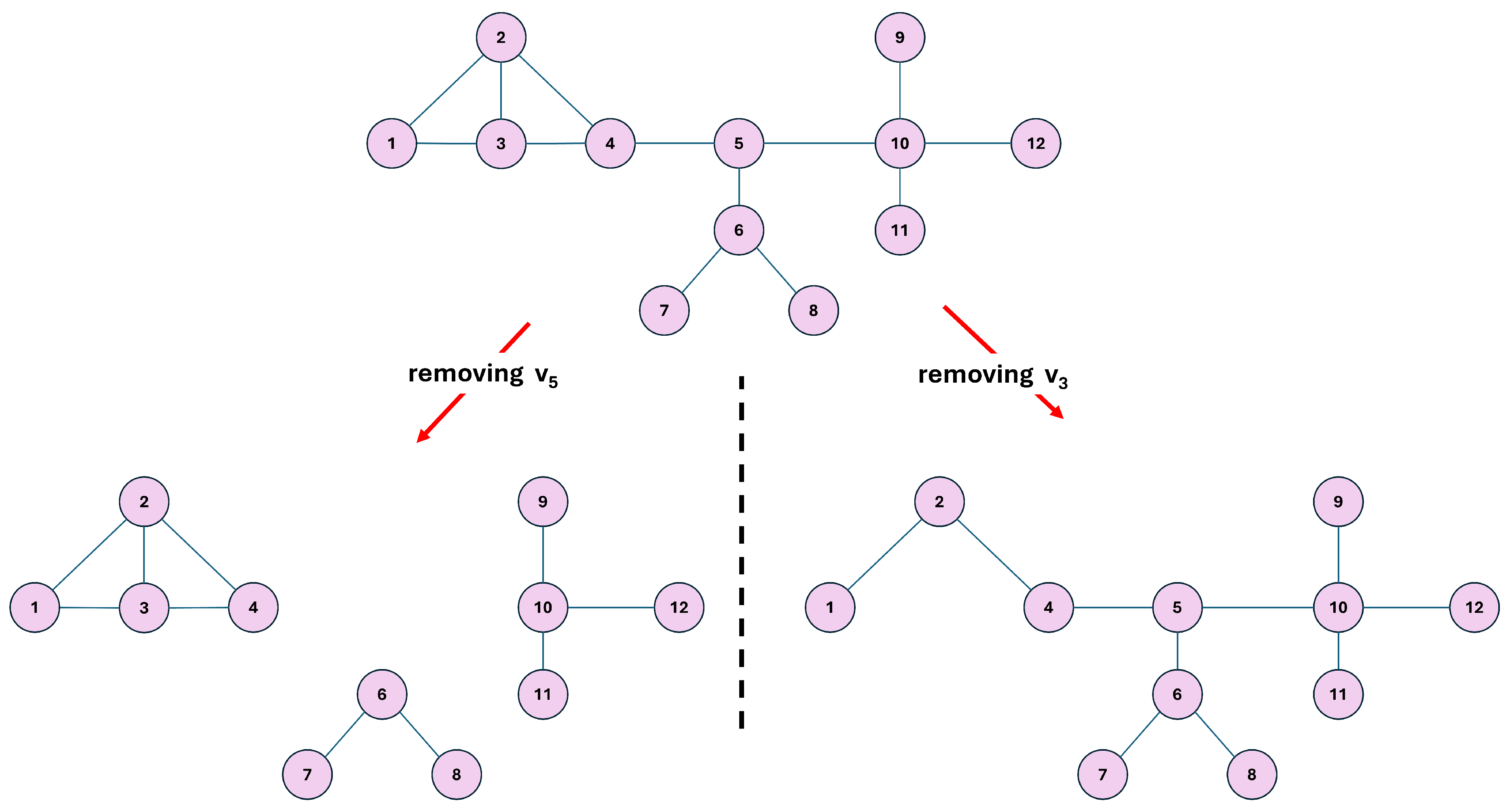
Figure 2.
Demonstrating the node removal and resulting networks based on Giu and Lao’s SE algorithm [64] (left branch), and the proposed ISE algorithm (right branch). Both algorithms detect as the most significant node, both with . According to the initial quantification of the SE algorithm, the second most significant node is with . Therefore, after removing the node, is removed. However, the proposed ISE algorithm re-evaluates the node significance after removing the node, finding as the most significant node with . Hence, according to ISE algorithm, after , not the node but node is removed.
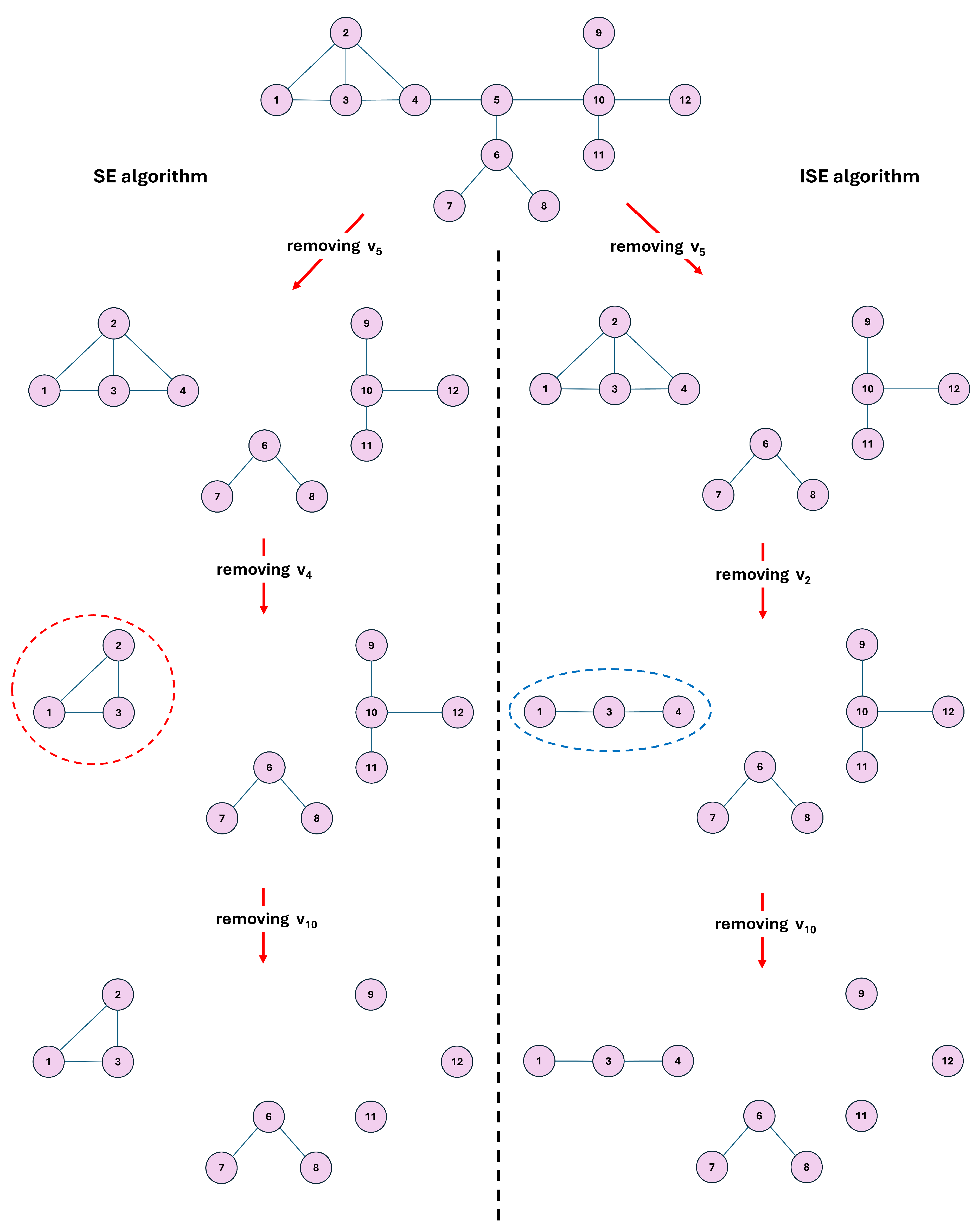
Figure 3.
Comparison of the SE and ISE algorithms based on Cumulative Structural Entropy (CSE) (left), and the size of the Largest Connected Component (LCC) (right) during iterative node removal for the network of Liu and Gao [64]. While SE accumulates increasing entropy values, ISE achieves faster entropy reduction due to dynamically updated significance scores. The LCC trends are mostly similar, with ISE showing a sharper fragmentation at one point, leading to a lower total LCC sum, achieving .
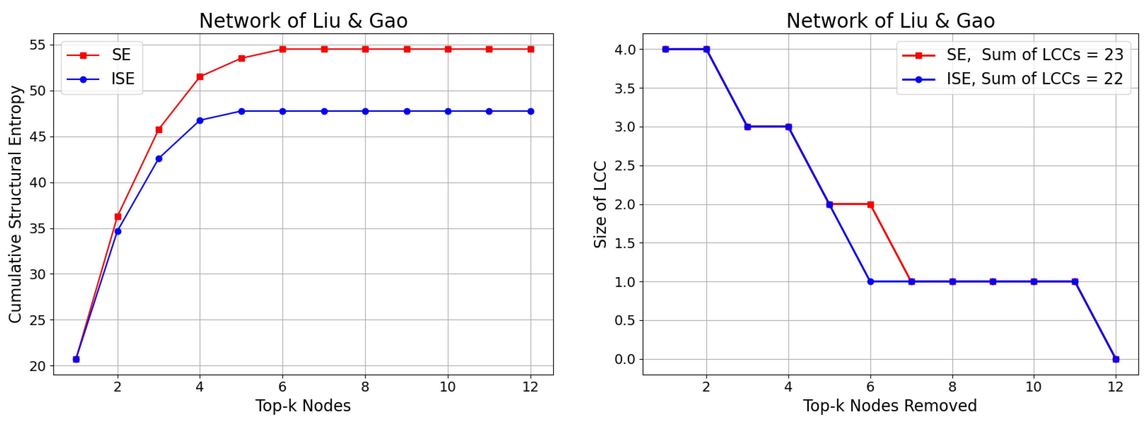
Figure 4.
Comparison of the SE and ISE algorithms based on Cumulative Structural Entropy (CSE) (left), and the size of the Largest Connected Component (LCC) (right) during iterative node removal for the Contiguous USA (CONT) network. While SE accumulates increasing entropy values, ISE achieves faster entropy reduction due to dynamically updated significance scores. The gap between SE and ISE in Size of LCC expands, achieving .
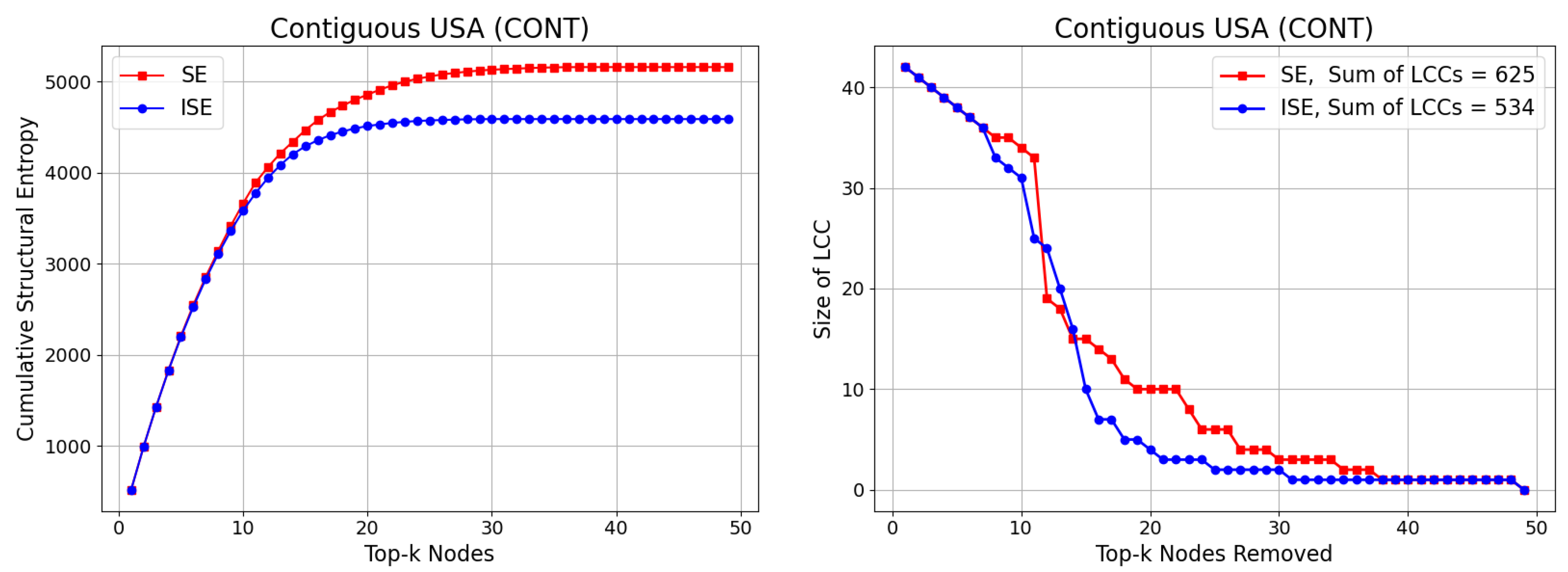
Figure 5.
Comparison of the SE and ISE algorithms based on Cumulative Structural Entropy (CSE) (left), and the size of the Largest Connected Component (LCC) (right) during iterative node removal for the Les Miserables (LESM) network. While SE accumulates increasing entropy values, ISE achieves faster entropy reduction due to dynamically updated significance scores. The gap between SE and ISE in Size of LCC is very similar to that of Contiguous USA (CONT) network, achieving .
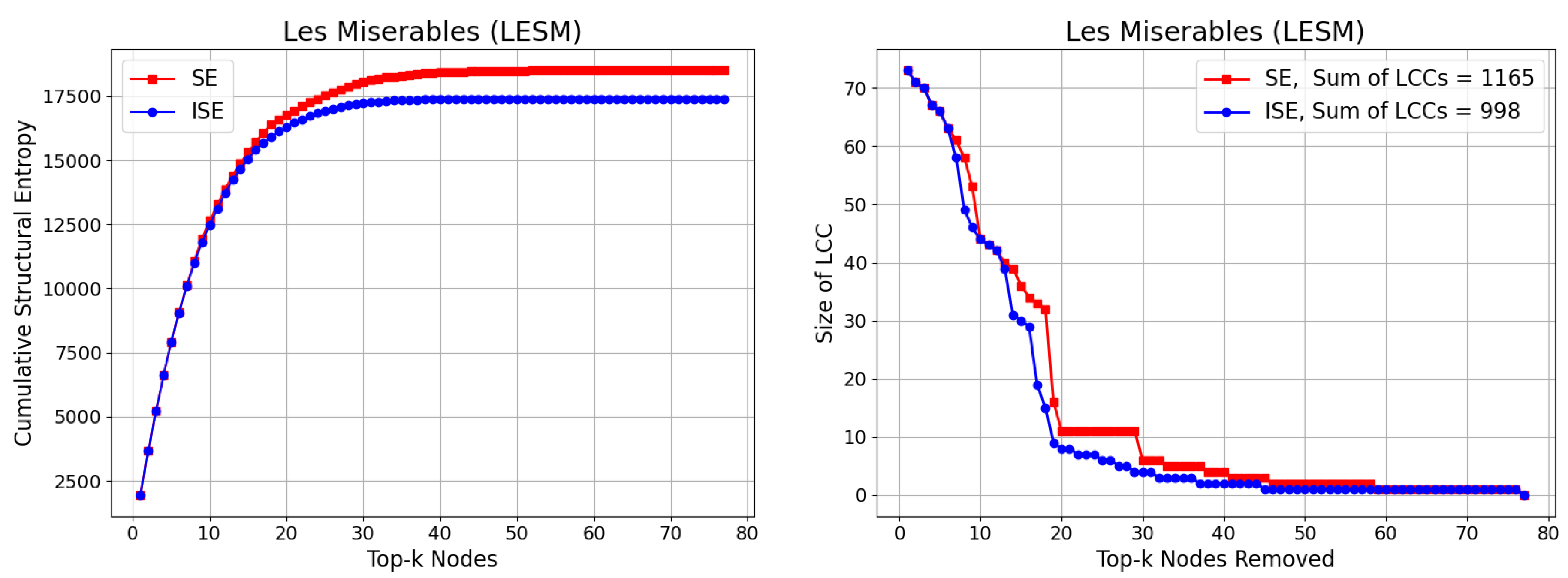
Figure 6.
Comparison of the SE and ISE algorithms based on Cumulative Structural Entropy (CSE) (left) and the size of the Largest Connected Component (LCC) (right) during iterative node removal for the Polbooks (POLB) network. While SE accumulates increasing entropy values, ISE achieves faster entropy reduction due to dynamically updated significance scores. The gap between SE and ISE in Size of LCC achieves .
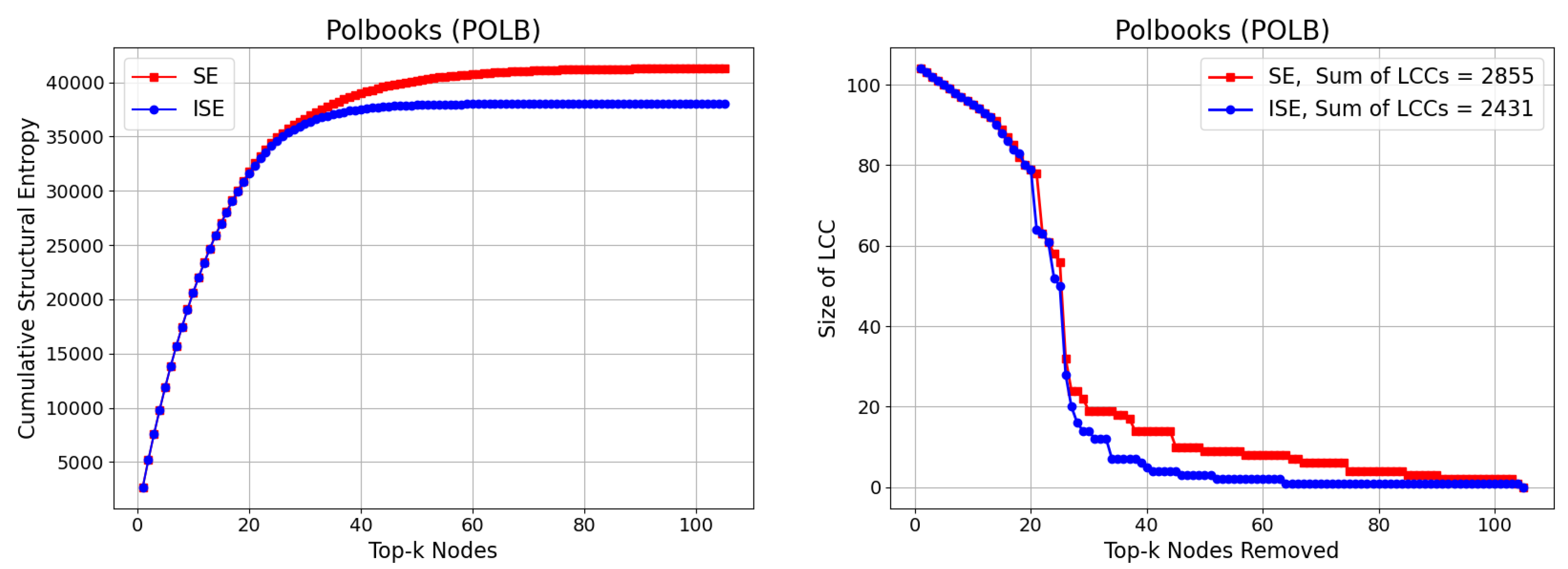
Figure 7.
Comparison of the SE and ISE algorithms based on Cumulative Structural Entropy (CSE) (left), and the size of the Largest Connected Component (LCC) (right) during iterative node removal for the Adjnoun (ADJN) network. While SE accumulates increasing entropy values, ISE achieves faster entropy reduction due to dynamically updated significance scores. The gap between SE and ISE is greater than the above networks, achieving .
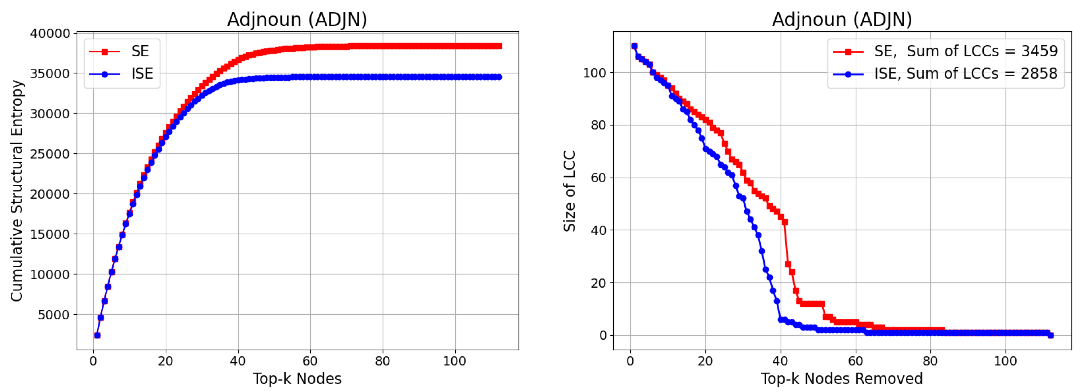
Figure 8.
Comparison of the SE and ISE algorithms based on Cumulative Structural Entropy (CSE) (left), and the size of the Largest Connected Component (LCC) (right) during iterative node removal for the Football (FOOT) network. While SE accumulates increasing entropy values, ISE achieves faster entropy reduction due to dynamically updated significance scores. The gap between SE and ISE in Size of LCC is slightly narrower than the previous networks, achieving .
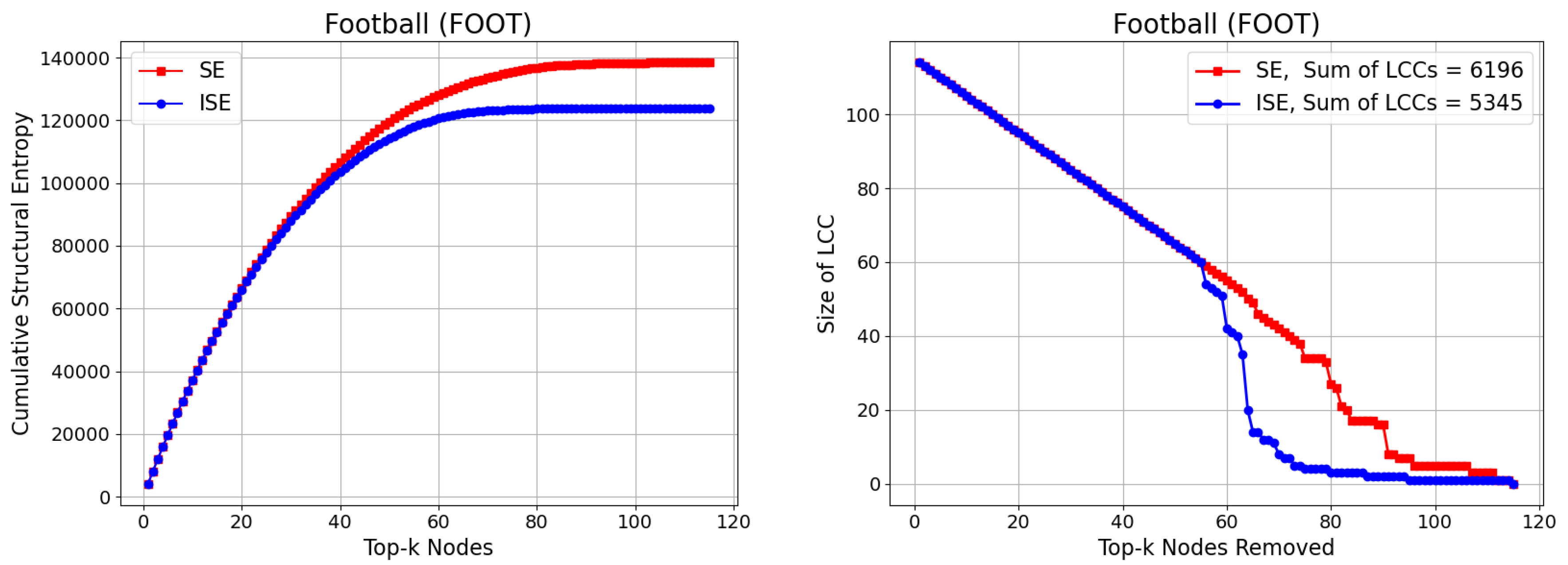
Figure 9.
Comparison of the SE and ISE algorithms based on Cumulative Structural Entropy (CSE) (left), and the size of the Largest Connected Component (LCC) (right) during iterative node removal for the Netscience (NETS) network. While SE accumulates increasing entropy values, ISE achieves faster entropy reduction due to dynamically updated significance scores. The gap between SE and ISE in Size of LCC is significantly wider than the previous networks, achieving .
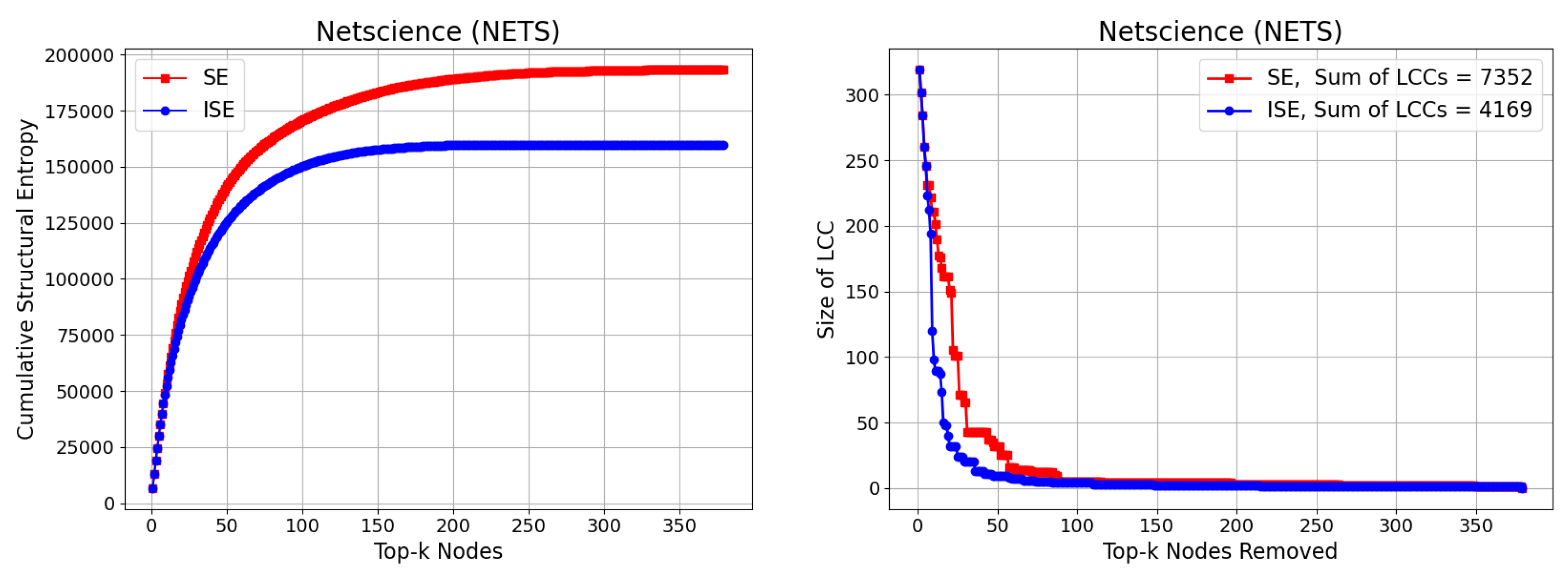
Figure 10.
Three-panel comparison on Network of Liu & Gao. Top: Average shortest-path length (ASPL) computed on the largest connected component (LCC) of the residual graph after removing k nodes. Middle: Diameter of the LCC. Bottom: Expected outbreak size (fraction of nodes in the percolated LCC) under bond percolation with , averaged over 100 independent realizations. Curves compare ISE (iterative SE; dynamic reordering) and SE.
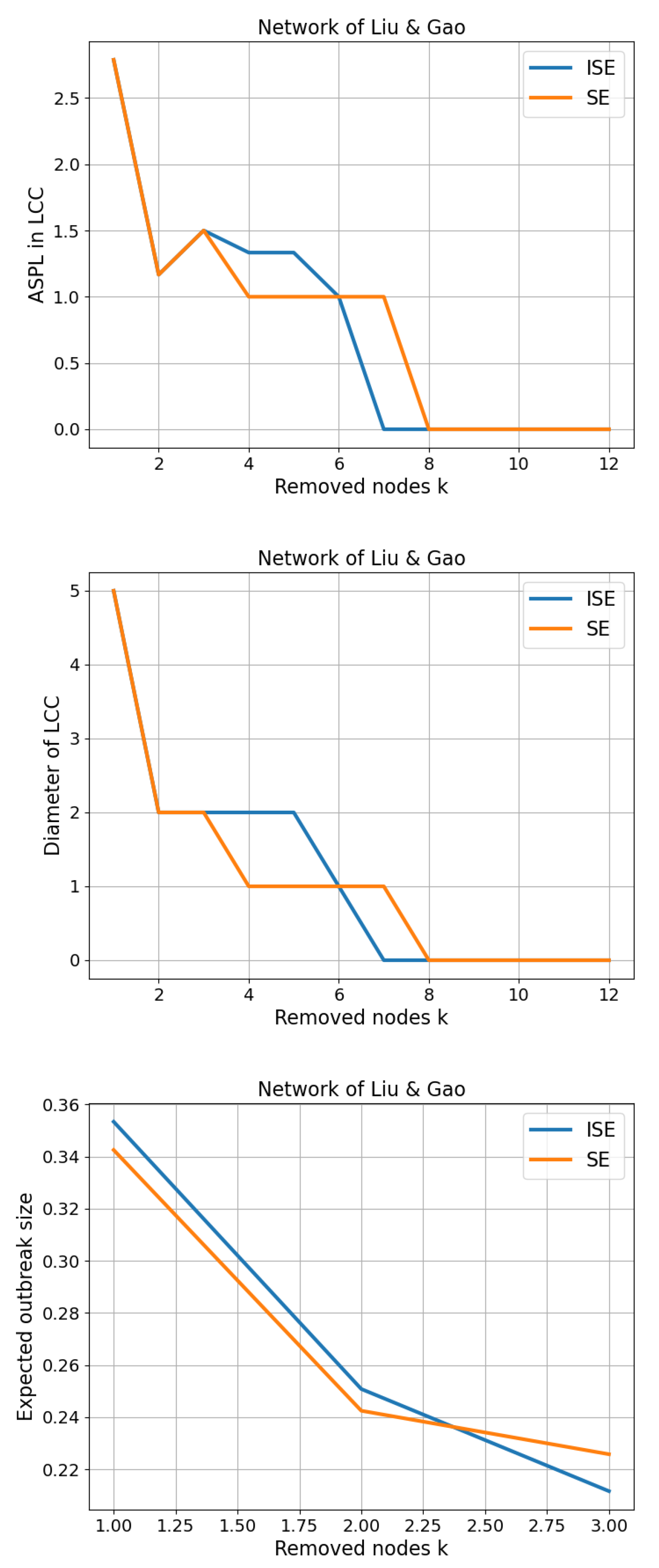
Figure 11.
Three-panel comparison on Contiguous USA (CONT) network. Top: Average shortest-path length (ASPL) computed on the largest connected component (LCC) of the residual graph after removing k nodes. Middle: Diameter of the LCC. Bottom: Expected outbreak size (fraction of nodes in the percolated LCC) under bond percolation with , averaged over 100 independent realizations. Curves compare ISE (iterative SE; dynamic reordering) and SE.
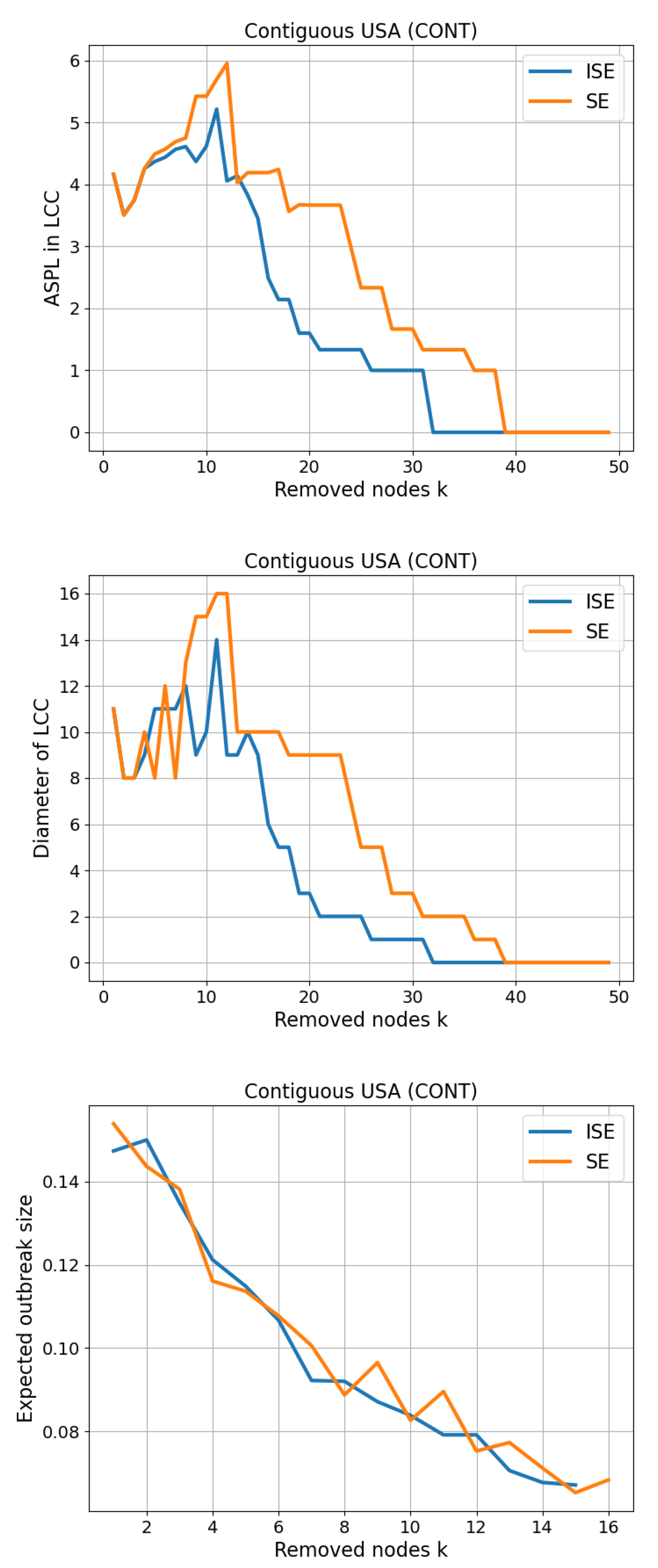
Figure 12.
Three-panel comparison on Les Miserables (LESM) network. Top: Average shortest-path length (ASPL) computed on the largest connected component (LCC) of the residual graph after removing k nodes. Middle: Diameter of the LCC. Bottom: Expected outbreak size (fraction of nodes in the percolated LCC) under bond percolation with , averaged over 100 independent realizations. Curves compare ISE (iterative SE; dynamic reordering) and SE.
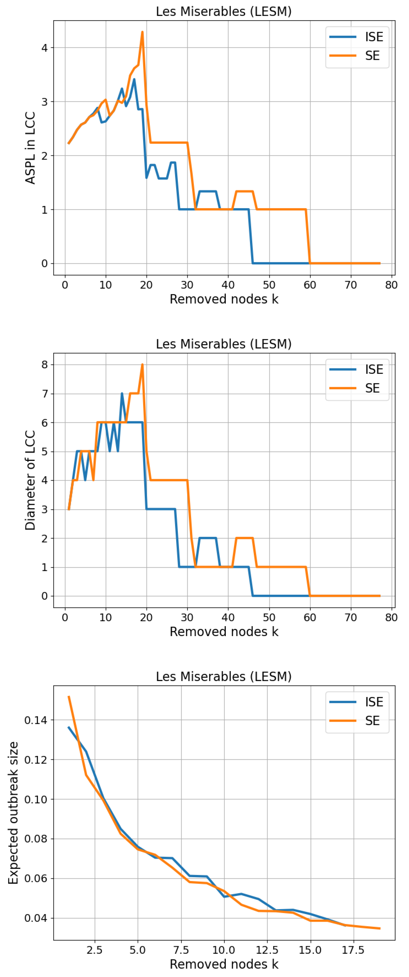
Figure 13.
Three-panel comparison on Polbooks (POLB) network. Top: Average shortest-path length (ASPL) computed on the largest connected component (LCC) of the residual graph after removing k nodes. Middle: Diameter of the LCC. Bottom: Expected outbreak size (fraction of nodes in the percolated LCC) under bond percolation with , averaged over 100 independent realizations. Curves compare ISE (iterative SE; dynamic reordering) and SE.
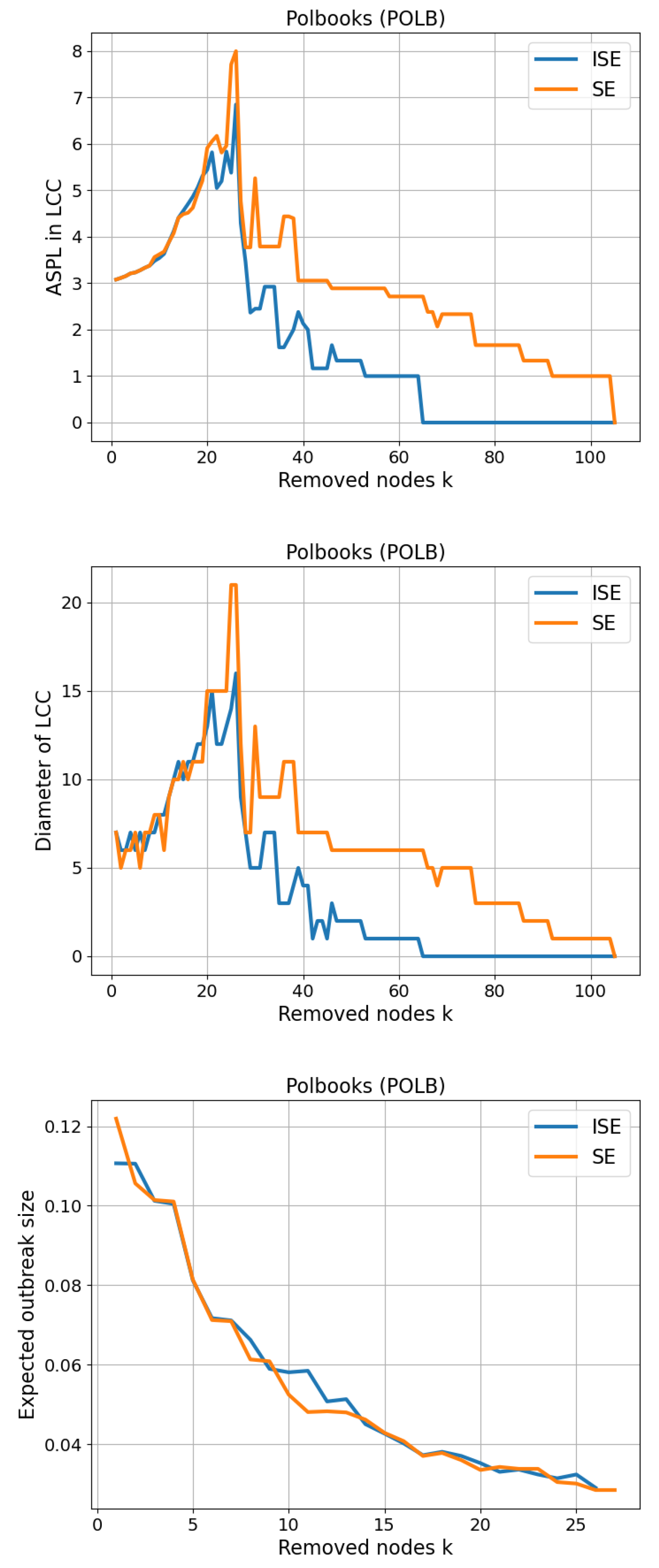
Figure 14.
Three-panel comparison on Adjnoun (ADJN) network. Top: Average shortest-path length (ASPL) computed on the largest connected component (LCC) of the residual graph after removing k nodes. Middle: Diameter of the LCC. Bottom: Expected outbreak size (fraction of nodes in the percolated LCC) under bond percolation with , averaged over 100 independent realizations. Curves compare ISE (iterative SE; dynamic reordering) and SE.
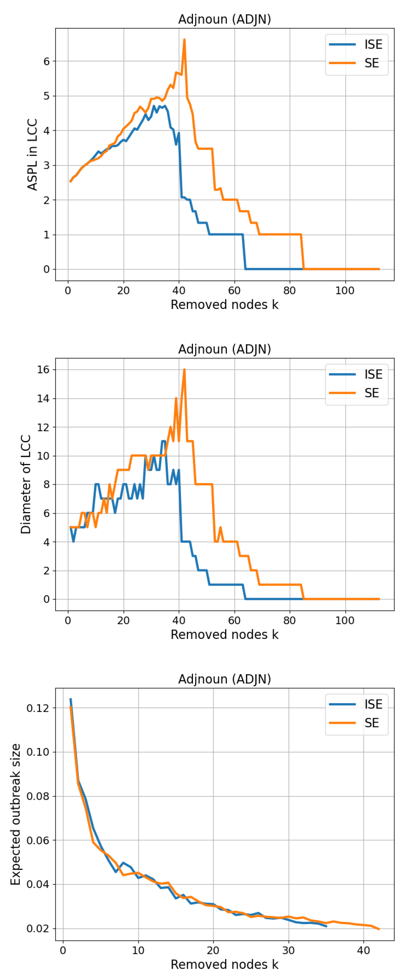
Figure 15.
Three-panel comparison on Football (FOOT) network. Top: Average shortest-path length (ASPL) computed on the largest connected component (LCC) of the residual graph after removing k nodes. Middle: Diameter of the LCC. Bottom: Expected outbreak size (fraction of nodes in the percolated LCC) under bond percolation with , averaged over 100 independent realizations. Curves compare ISE (iterative SE; dynamic reordering) and SE.
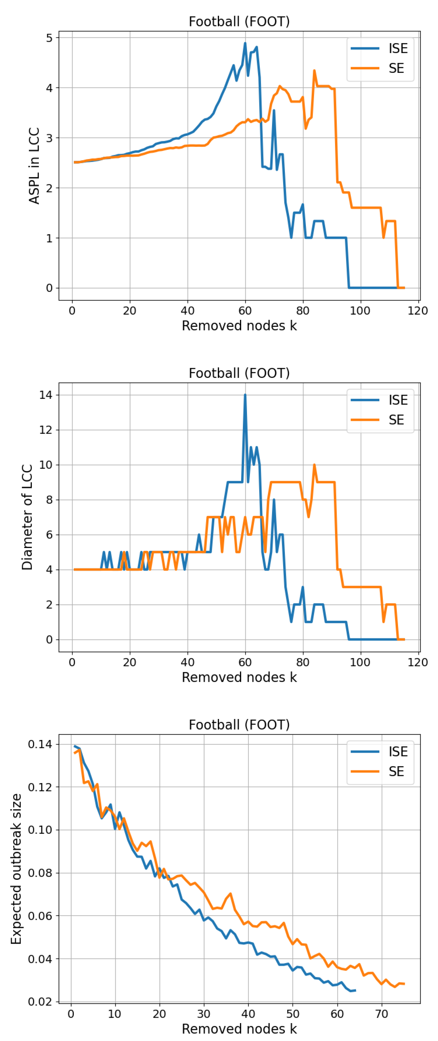
Figure 16.
Three-panel comparison on Netscience (NETS) network. Top: Average shortest-path length (ASPL) computed on the largest connected component (LCC) of the residual graph after removing k nodes. Middle: Diameter of the LCC. Bottom: Expected outbreak size (fraction of nodes in the percolated LCC) under bond percolation with , averaged over 100 independent realizations. Curves compare ISE (iterative SE; dynamic reordering) and SE.
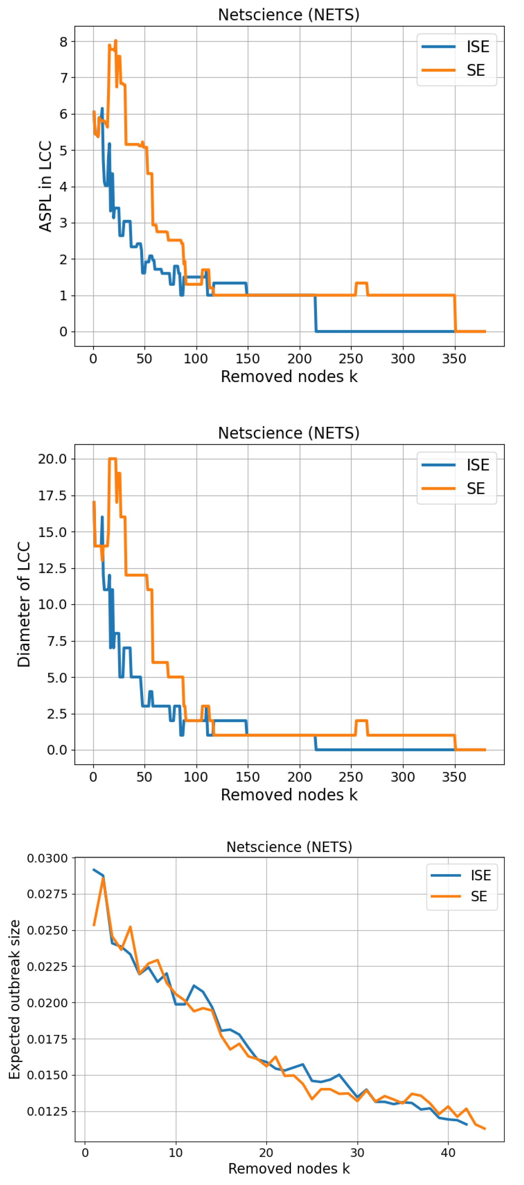

Table 1.
Structural entropies of nodes based on the single-shot quantification of SE algorithm, and the iterative quantification of ISE algorithm.
Table 1.
Structural entropies of nodes based on the single-shot quantification of SE algorithm, and the iterative quantification of ISE algorithm.
| SE | ISE |
|---|---|
Table 2.
Monotonicity value M for various ranking methods.
| Dataset | M(DC) | M(IKS) | M(WR) | M(SE) | M(ISE) |
|---|---|---|---|---|---|
| Liu & Gao | 0.573 | 0.669 | 0.799 | 0.854 | 1.000 |
| CONT | 0.697 | 0.794 | 0.954 | 1.000 | 1.000 |
| LESM | 0.904 | 0.894 | 0.993 | 0.994 | 1.000 |
| POLB | 0.825 | 0.838 | 0.996 | 1.000 | 1.000 |
| ADJN | 0.866 | 0.874 | 0.996 | 0.999 | 1.000 |
| FOOT | 0.363 | 0.941 | 0.928 | 1.000 | 1.000 |
| NETS | 0.764 | 0.761 | 0.983 | 0.995 | 1.000 |
Disclaimer/Publisher’s Note: The statements, opinions and data contained in all publications are solely those of the individual author(s) and contributor(s) and not of MDPI and/or the editor(s). MDPI and/or the editor(s) disclaim responsibility for any injury to people or property resulting from any ideas, methods, instructions or products referred to in the content. |
© 2025 by the authors. Licensee MDPI, Basel, Switzerland. This article is an open access article distributed under the terms and conditions of the Creative Commons Attribution (CC BY) license (http://creativecommons.org/licenses/by/4.0/).
Copyright: This open access article is published under a Creative Commons CC BY 4.0 license, which permit the free download, distribution, and reuse, provided that the author and preprint are cited in any reuse.


