
Submitted:
17 August 2025
Posted:
18 August 2025
You are already at the latest version
Abstract
Wireless communication applications above 300 GHz need careful analog electronics design that takes into account the frequency-dependent nature of ohmic resistance at these frequencies. The cumbersome development of electronics brings quantum optical communication solutions for the sixth generation (6G) THz band located between 300 GHz and 10 THz into focus. In this manuscript, the authors propose to replace the classical radio frequency based inner physical layer transceiver blocks used in classical channel coded short range wireless communication systems by wireless quantum optical communication concepts. Besides discussing the resulting generic concept of the wireless quantum optical communications and illustrating optimum quantum data detection schemes, novel reduced state quantum data detection and novel Kohonen maps based quantum data detection, will be addressed. All the considered quantum data detection schemes provide soft outputs required for the lowest possible block error ratio (BLER) at the output of the channel decoding. Furthermore, a novel polar codes design approach determining the polar sequence by appropriately combining already available polar sequences tailored for low BLER is presented for the first time after illustrating the basics of polar codes.
In addition, turbo equalization for wireless quantum optical communications using polar codes will be presented, for the first time explicitly stating the generation of soft information associated with the codebits and introducing a novel scheme for the computation of extrinsic soft outputs to be used in the turbo equalization iterations. New simulation results emphasize the viability of the theoretical concepts.
Keywords:
6G
; Kohonen maps based quantum data detection
; log-likelihood ratio (LLR)
; optimum quantum data detection
; polar codes
; polar code design
; polar sequence
; reduced state quantum data detection
; soft outputs
; turbo equalization with polar codes
; wireless quantum optical communications
1. Introduction
Recent studies [1] have illustrated that radio applications operating above , which is approximately equal to that particular natural frequency at the low end of the far infrared radiation [2][Table E1-1, p. 208], [3], require meticulous analog design. This is due to the frequency-dependent behavior of ohmic resistance at such high frequencies [1], which brings optical communication solutions for the sixth generation (6G) THz band into sharp focus. Following the experimental demonstration of quantum supremacy [4], there has been a significant surge of interest in wireless quantum optical communication concepts. These aim to replace conventional radio frequency-based transceivers at the inner physical layer of classical channel coded wireless systems. Generally, quantum communications means the transmission of classical information over a quantum channel, where the information is encoded in quantum states [5,6,7]. In future generations of wireless communication systems, the aforementioned growing popularity may suggest the replacement of mixed signal and analog components in the transceivers for mobile radio systems by components relying on quantum optics.
The basic block diagram of the resulting physical layer transmission, originating at a single transmitter located e.g. at a base station, usually called eNB, and terminating at a single receiver located consequently at the user equipment (UE), is shown in Figure 1, cf. e.g. [8][Fig. 1.30, p. 289]. The transmitter consists of the classical channel encoder, which has been common in classical wireless communication systems, cf. e.g [8], and a quantum transmitter, which represents the classical information generated by the classical channel encoder by a sequence quantum states. In this communication, we will focus on sophisticated channel coding based on polar codes, cf. e.g. [8][Chapter 4, pp. 336-388] for a brief introduction. The quantum transmitter can e.g. be realized by a quantum mechanical harmonic oscillator that provides coherent states, namely a laser [5][pp. 11, 80f.], [6][p. 1584], [9][pp. 125-128], which will be considered in this communication. The quantum channel, which conveys the information generated by the transmitter to the single receiver, is connected to the output of the quantum transmitter and to the input of the receiver, which consists of a quantum receiver followed by a classical channel decoder. The quantum receiver is supposed to be a soft output quantum data detector that consists of the measurement device, characterized by commuting measurement operators, and the soft output generation unit, which uses the measured probability values to create soft outputs in the form of log-likelihood ratios (LLRs). The mode of operation of the wireless quantum optical communication system depicted in Figure 1 will be addressed in Section 2.
Figure 1.
Wireless quantum optical communication system with classical channel coding, cf. also [8][Fig. 1.30, p. 289].
Figure 1.
Wireless quantum optical communication system with classical channel coding, cf. also [8][Fig. 1.30, p. 289].
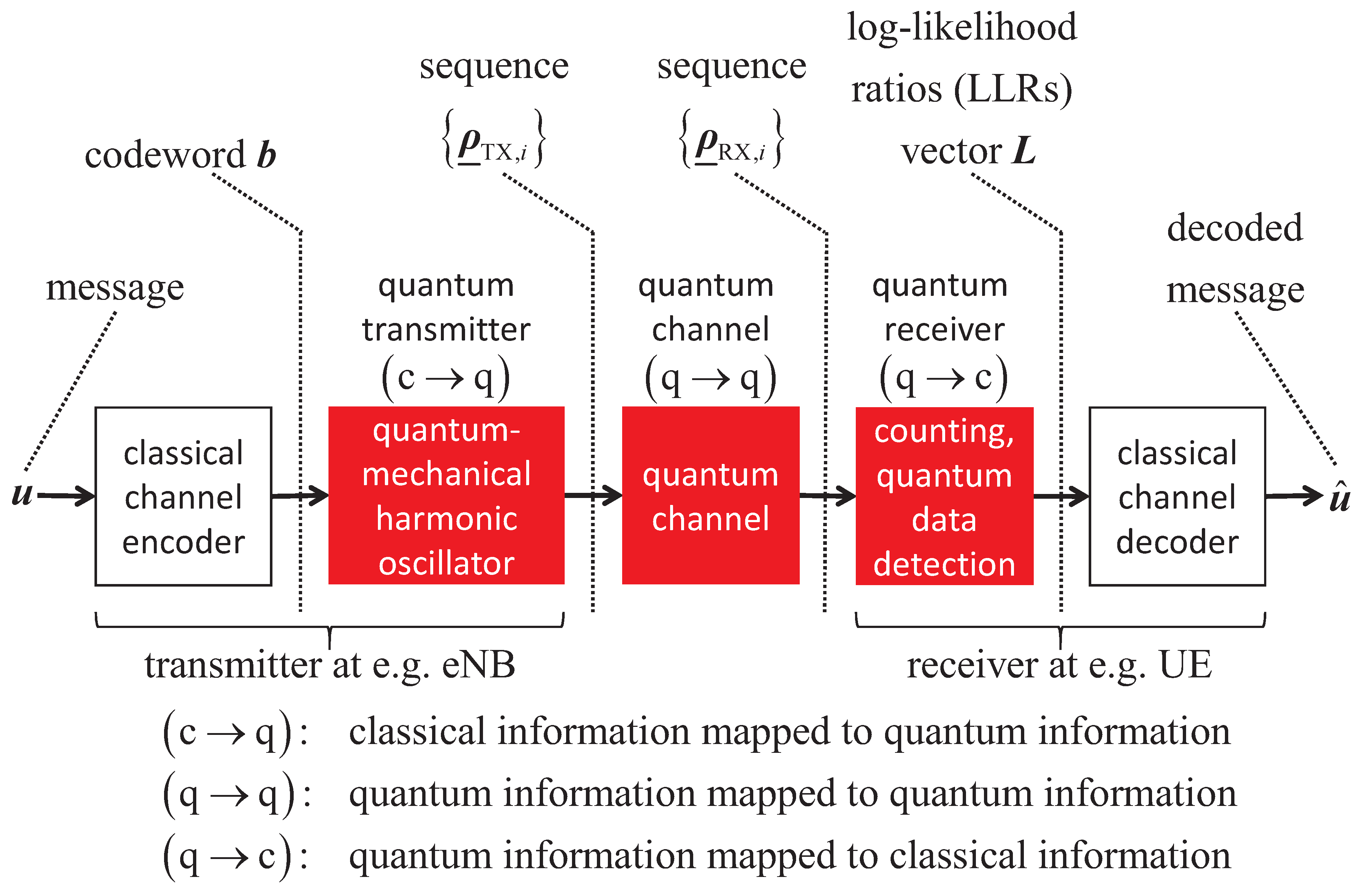
Every communication system must be tailored to the physical conditions presented by the transmission channel. In the context of short range communication links, which are typical for e.g. IEEE 802.11 “Wireless Local Area Network” (802.11/WLAN) standard [10], recently amended to accommodate light communications [11] in a similar manner discussed in e.g. [12], and for the anticipated short range wireless optical solutions, becoming increasingly important in the context of 6G wireless communications, cf. e.g. [13], we may suppose that the quantum channel has one single path, thus being memoryless, and the transmission is subject to little environmental interaction, i.e. negligible scattering and turbulence, therefore, neglecting any decoherence [14,15,16]. Since the received radiation field may contain a coherent signal, emitted by the quantum mechanical harmonic oscillator in the case it is on and superimposed by the omnipresent thermal radiation field [6,9,17] the statistical operator of the received radiation field given in the basis of the number states may not be diagonal, having unvanished coherences, i.e. interference terms, which are the off-diagonal elements of the matrix representation of the said statistical operator, cf. also [14][p. 34]. However, in e.g. the case of unknown random carrier phases [9][pp. 171f.], the said coherences will approach zero always yielding a diagonal statistical operator in the basis of the number states, cf. also [14][pp. 88-93].
In the context of mobile communications, however, wireless communication links typically suffer from multipath propagation with uncorrelated scattering, cf. e.g. [17,18], which will hold true for the quantum channel, as well [19,20,21]. Similar to mobile communications, intersymbol interference (ISI) at the quantum receiver depicted in Figure 1 must be expected, which had not been discussed earlier than [19]. We will illustrate this still novel corresponding quantum mechanical system model in Section 2, considerably extending the presentation of [19], by setting out from the quantum mechanical communication theory known for single path transmission [6,9,17]. Also, soft output quantum data detection, mitigating the effect of ISI will be treated in Section 2. Besides the discussion of optimum quantum data detection with soft outputs, a novel soft output reduced state quantum data detection approach will be introduced for the first time. In addition, the authors will propose a novel soft output Kohonen maps based quantum data detection for the first time, which extends a concept recently introduced for the data detection in classical mobile communications [22].
In Section 3 polar coding will be addressed, by briefly illustrating its general concept and also by introducing a detailed design strategy for the first time summarized in e.g. Algorithm 2, yielding an appropriately chosen polar sequence for wireless quantum optical communications. In addition, applying polar codes in turbo equalization, explicitly stating, seemingly for the first time, the creation of the required soft outputs for the codebits, and introducing two viable novel methods for the analytically closed generation of the extrinsic soft outputs to be used in the turbo equalization iterations, will be discussed for the first time in Section 3.
Section 4 reports obtained performance results, showing the feasibility and the viability of the concepts suggested in this manuscript. Section 5 concludes the manuscript.
In what follows, complex values are underlined and denotes complex conjugation. Operators, matrices and vectors are in bold face italics. equal to denotes the Galois field with the two elements 0 and 1. equal to is the set of nonnegative integers and equal to denotes the set of positive integers. equal to , , is the set of message bit indices and equal to , , , is the set of codebit indices. We will apply the Dirac notation.
2. Quantum Mechanical System Model
2.1. Initial Considerations
Since the wireless quantum optical communication system model considered by the authors and sketched in e.g. Figure 1 bears considerable novelty, first being addressed in recent publications such as e.g. [20,21,23], the authors will illustrate its mode of operation in this Section 2 to facilitate an easy access by the reader.
2.2. Transmitter
Let us begin with the transmitter, cf. Figure 1. Suppose that messages containing message bits , , are to be transmitted. To improve protection against transmission errors, the said messages are encoded by the classical channel encoder, generating the codewords with , , codebits , . denotes the codebit period of a codebit prevailing in a time interval , leading to the total transmission period of .
Next, the N codebits , , are transmitted via a device converting this classical information into quantum states. Analog to conventional antennas that generate an electromagnetic field in a coherent state [6][p. 1584], we will use a laser [5][pp. 11, 80f.], [6][p. 1584], [9][pp. 125-128]. Any codebit , , modulates the laser as follows. The laser light is turned on if the present codebit is equal to 1 and off if the present codebit is equal to 0. This simple modulation scheme is termed on-off keying (OOK) [5][pp. 11, 318-320], [17][pp. 435-446].
Suppose that only a single mode with a fixed angular frequency is used for communication purposes. With the number states , , the coherent state of the radiation field emitted by the laser and associated with the ith codebit , having the complex amplitude , , is given by the coherent state vector [5][pp. 80, 479f.]
If equals 0, the emitted radiation field is in its ground state and contains no signal photons. On the other hand, if equals 1 the number of signal photons in the radiation field represented by the above coherent state given in (1) follows a Poisson distribution with the mathematical expectation equal to . It is assumed that the modulus remains constant throughout the entire transmission duration , see also [9, eq. (2.17), p. 125].
Although the coherent state described in (1) is not stationary over an observation time interval of duration , any time dependence within the ith observation time interval, characterized by the angular frequency and the initial phase angle , is entirely captured by the phase factor in , because the magnitude is assumed to remain constant [9, pp. 125, 171]. Therefore, apart from a phase factor, the number state stays constant throughout the observation time interval .
2.3. Short Range Transmission via a Single Path Quantum Channel
As previously noted in Section 1, we will first consider the transmission occuring via a single path quantum channel, where the received radiation field consists of the coherent signal emitted by the aforementioned laser, superimposed with the ever present thermal radiation field [6,9,17]. This situation was recently illustrated in [23, Sect. II], which forms the foundation of the following illustration. Due to the short range nature of the link and the relatively weak thermal radiation field, the interaction between the coherent signal and the surrounding environment remains minimal.
Let represent the complex amplitudes of the coherent states comprising the thermal radiation field, and let equal to denote the average number of thermal noise photons. Then, during the observation time interval , , the statistical operator in Glauber’s “P-representation” is given by [9, eqs. (4.6) and (4.10), pp. 134f.]
Given the Boltzmann constant , the temperature T, and the reduced Planck constant ℏ, the average number of thermal photons is determined by the Planck distribution law [9,17]
Let denote the associated Laguerre polynomial of degree n [24], and let the standard Laguerre polynomial of degree n, written as , be defined as [24]. Also, let denote the factorial of . Assuming is the average number of signal photons present in the coherent radiation field emitted by the laser when equals 1, i.e., when the laser is active, and is the average number of thermal photons present in the thermal radiation field, and computing in the number state basis , the matrix element in the nth row and mth column of the matrix representation of as defined in (2) is given by
in the case where , that is, within the upper triangular submatrix including the main diagonal of the said matrix representation of , cf. e.g. [9,17] for a similar representation. For the case where , corresponding to the strict lower triangular submatrix excluding the main diagonal of the matrix representation of , we obtain
see also e.g. [9,17].
When a nonvanishing coherent signal is present in the received radiation field, that is, when equals 1, equations (4) and (5) reveal the existence of nonzero interference terms called coherences, indicated by the nonzero off-diagonal elements of . Clearly, corresponds to a scenario without decoherence and with a known carrier phase of the quantity appearing in (4). Since is an observable and, thus, a Hermitian operator, it admits a diagonalization, yielding a complete orthonormal system of eigenkets that constitute a new basis of the Hilbert space, distinct from the number state basis.
If decoherence, an unknown carrier phase, or both dominate the transmission scenario, the phase of the quantity has to be revisited. The said phase, which is then appropriately modelled as a uniformly distributed random variable, must be averaged out during the data detection process. As a result, all interference terms, that is, all off-diagonal elements in the matrix representation of with respect to the number state basis, vanish. The resulting statistical operator then becomes diagonal, having the matrix representation [9]
When the coherent signal is absent, i.e., when equals 0, equation (2) simplifies to [9,17]
representing the Bose-Einstein distribution of thermal photons within the thermal radiation field. Clearly, is diagonal when expressed in the number state basis, which therefore forms the set of its eigenkets. Then, no interference terms, i.e., no coherences, are present, indicating that the carrier phase of the thermal radiation is unknown and can be accurately modelled as a uniformly distributed random variable.
According to (4) as well as (5) and (7), the operators and possess different eigenstates and therefore do not commute. In contrast, from (6) and from (7) share the same complete orthonormal system of eigenkets, namely, the number states, and are thus compatible. These observations govern the design of the optimum soft output quantum data detector.
Since the considered quantum channel has one single path, no memory effects need to be taken into account when designing the optimum quantum data detector. Therefore, quantum data detection can be performed independently within each observation time interval.
We begin with the ith observation time interval , supposing that equal to 0 and equal to 1 are equally probable. Using the Kronecker delta , and defining the cost equal to for deciding in favor of hypothesis when the transmitted codebit had the value m, where , under the maximum a-posteriori probability (MAP) concept [17, eq. (3.1181), p. 433], and considering the Hermitian measurement operator corresponding to hypothesis , the average cost of the measurement strategy during the ith observation time interval is given by [9, eq. (1.3), p. 90]
Let be the eigenkets and , , the corresponding real eigenvalues of the Hermitian detection operator
The optimum measurement operators are then given by [6,9]
and
If the measurement at the input of the quantum receiver, represented by the trace of , yields the eigenstate with eigenvalue , the detected codebit is equal to 1. Otherwise, the detected codebit is equal to 0. Similarly, if the measurement represented by the trace of yields the eigenstate with eigenvalue , the detected codebit is equal to 1. Otherwise, it is equal to 0. Therefore, with
the optimum soft output in the ith observation time interval is hence represented by the LLR
Using the sign function , the MAP detection rule applied by the optimum soft output quantum data detector is expressed as
2.4. Multipath Transmission and Reception with Decoherence
In particular, scenarios involving longer transmission links often experience multipath transmission and reception. In such cases, the quantum channel is characterized by multiple paths, through which the transmitted signals arrive at the receiver. This situation has been illustrated very recently for the first time, cf. e.g. [19,20,21].
Consider a quantum channel modelled as a linear multipath channel that causes uncorrelated scattering of the signal photons emitted by the laser. These scatterers are randomly located and statistically independent, forming a continuum of uncorrelated scatterers similar to what occurs in mobile propagation channels [18,19]. The channel impulse response (CIR) of this multipath channel, parameterized by the delay , is denoted as [19]. We assume that the CIR is nonzero only for within the delay time interval , where . Under these conditions, ISI arises at the quantum receiver. Defining
the said multipath channel is referred to as a -path channel. The signal arriving at the receiver can be expressed by the ket vector [19]
The previously mentioned uncorrelated scattering induces decoherence [14,15,16,25], which contributes to the loss of phase coherence between the transmitter and the receiver, see e.g. [19,20,21]. As a result, we should assume that no phase coherence is preserved between the transmitter and receiver [6][p. 1590], [9,19][p. 171]. Consequently, the zero phase angles appearing in the aforementioned phase factors mentioned in Section 2.2 are considered unknown and modelled as uniformly distributed random variables with the constant probability density function of . Moreover, the uncorrelated scattering inherent to the multipath quantum channel further contributes to the degradation of phase coherence, cf. e.g. [19] and the references therein.
In the absence of phase coherence, the optimum quantum receiver employs photon counting at its front end [6][p. 1590]. Assume that the transmitter and the receiver are synchronized in time, meaning that the quantum receiver operates over mutually disjoint and consecutive observation time intervals of duration , each beginning with the arrival of the corresponding codebit [19]. Using the number operator and denoting mathematical expectation by , the average number of signal photons received during the observation time interval is given by , after averaging over all uniformly distributed phase differences , and we obtain
Due to decoherence and averaging over , the second integral vanishes, while the first integral remains unaffected. Therefore, equation (19) simplifies to [19]
which becomes
supposing that only channel coefficients , , can assume nonzero values.
In the case of a single path channel where equals 1, only the first term of equation (21) remains. The scenario where equals 1 has already been discussed, for instance, in [6, pp. 1589f] and [9, pp. 171-176]. Moreover, if is a nonnegative random variable with unit expected value, the result is a fading single path turbulent channel, also known as a turbulence channel, which was already investigated from a quantum communications perspective several decades ago [26][pp. 1630-1644].
For , the ISI term in equation (21) does not vanish [19]. As a result, the average number of received signal photons of (21) depends not only on the current codebit , but also on the preceding codebits , …. Therefore, equation (21) describes a finite state machine (FSM) that operates according to a Markov chain model [17,19,27].
In the context of Mealy modelling, cf. e.g. [27], the previously described FSM consists of states , defined as at each time index . Since the term can take on either of two distinct values, 0 or , each of the states gives rise to two transitions, labelled by the hypothetical codebit value . This results in a total of distinct transitions, which lead to the states at the next time step [19]. The behavior of the said FSM is conveniently represented by a trellis diagram, often abbreviated as trellis [17,19,28]. Accordingly, the possible transitions correspond to the different values that the average number of received signal photons , as defined in (21), can assume during each observation time interval , with . For this reason, we will denote as going forward, identifying these quantities as the distinct hypotheses employed in the quantum data detection scheme [19]. Note that the said hypotheses do not necessarily match the actual number of received signal photons observed in the ith observation time interval [19].
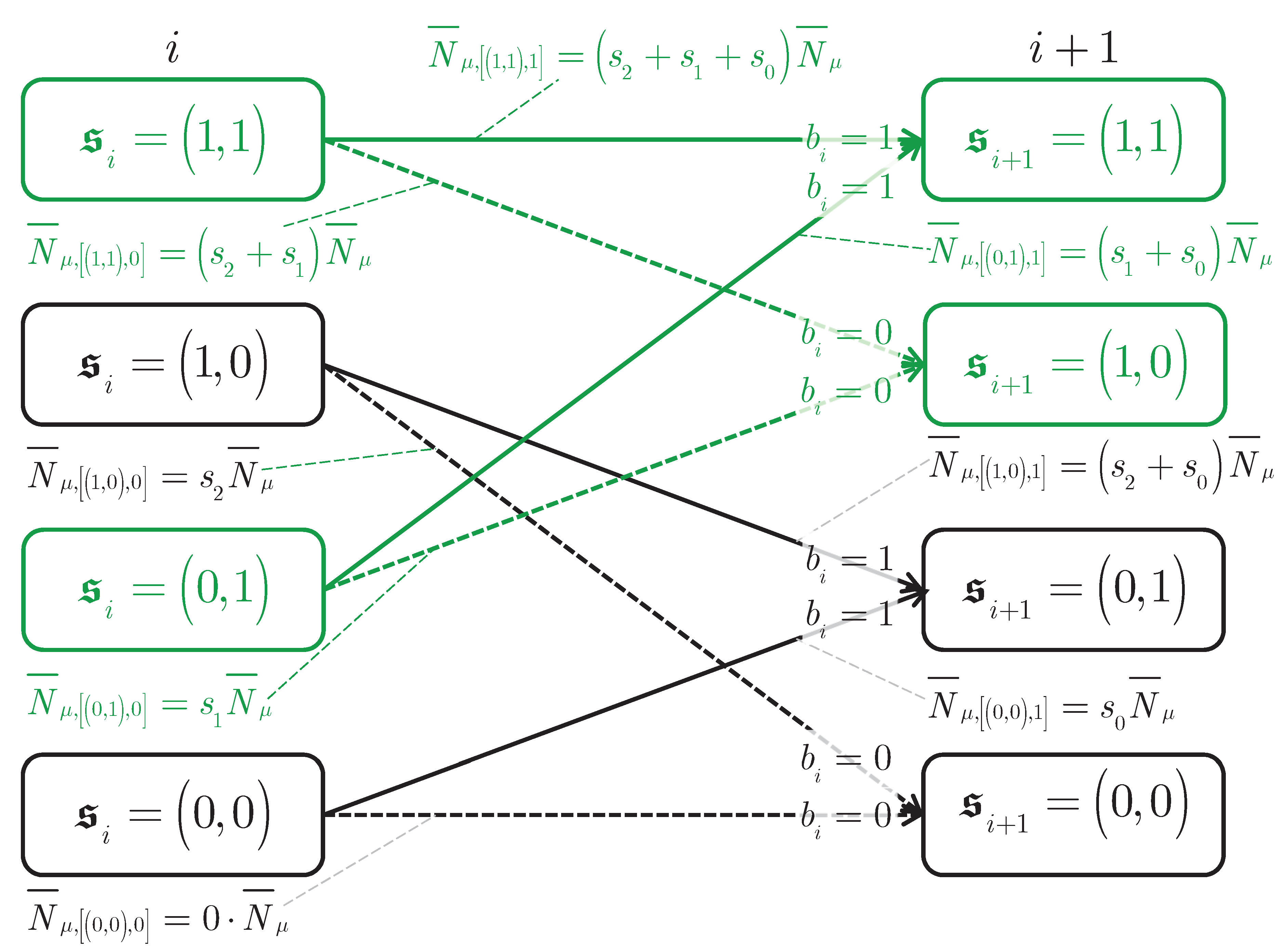
Figure 2 shows the detail of a trellis representing a quantum channel with equal to 3 possibly nonvanishing channel coefficients , and , thus, when applying Mealy modelling, having equal to 4 states at each time instant. The two states equal to and equal to at time instant i are connected to the two states equal to and equal to at time instant by a total of equal to four transitions. The said states and the aforementioned four transitions, all represented in black color, form the first of the two butterflies of the considered trellis. The two states equal to and equal to at time instant i are connected to the two states equal to and equal to at time instant by a total of equal to four transitions. These states and the associated four transitions, all represented in green color, form the second of the two butterflies of the considered trellis.
Figure 2.
Detail of a trellis representing a quantum channel with equal to 3 possibly nonvanishing channel coefficients , and , thus, when applying Mealy modelling, having equal to 4 states at each time instant; the two states equal to and equal to at time instant i are connected to the two states equal to and equal to at time instant by a total of equal to four transitions, forming the first of the two butterflies; the two states equal to and equal to at time instant i are connected to the two states equal to and equal to at time instant by a total of equal to four transitions, forming the second of the two butterflies; on-off keying (OOK) is assumed.
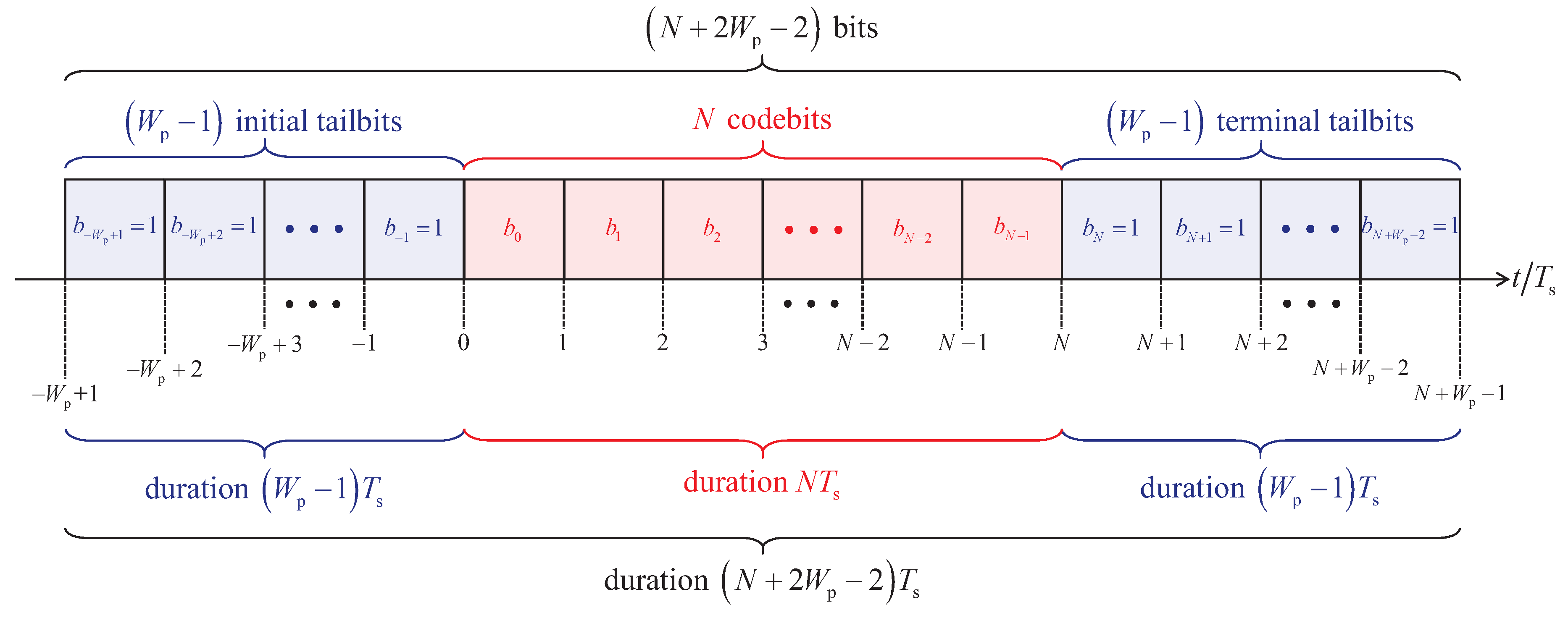
To support trellis initialization in the state equal to and trellis termination in the state equal to , a choice known to improve data detection performance, we introduce initial and terminal tailbits. Specifically, we set equal to 1 for all . All other codebits , for and , are assumed to be 0.
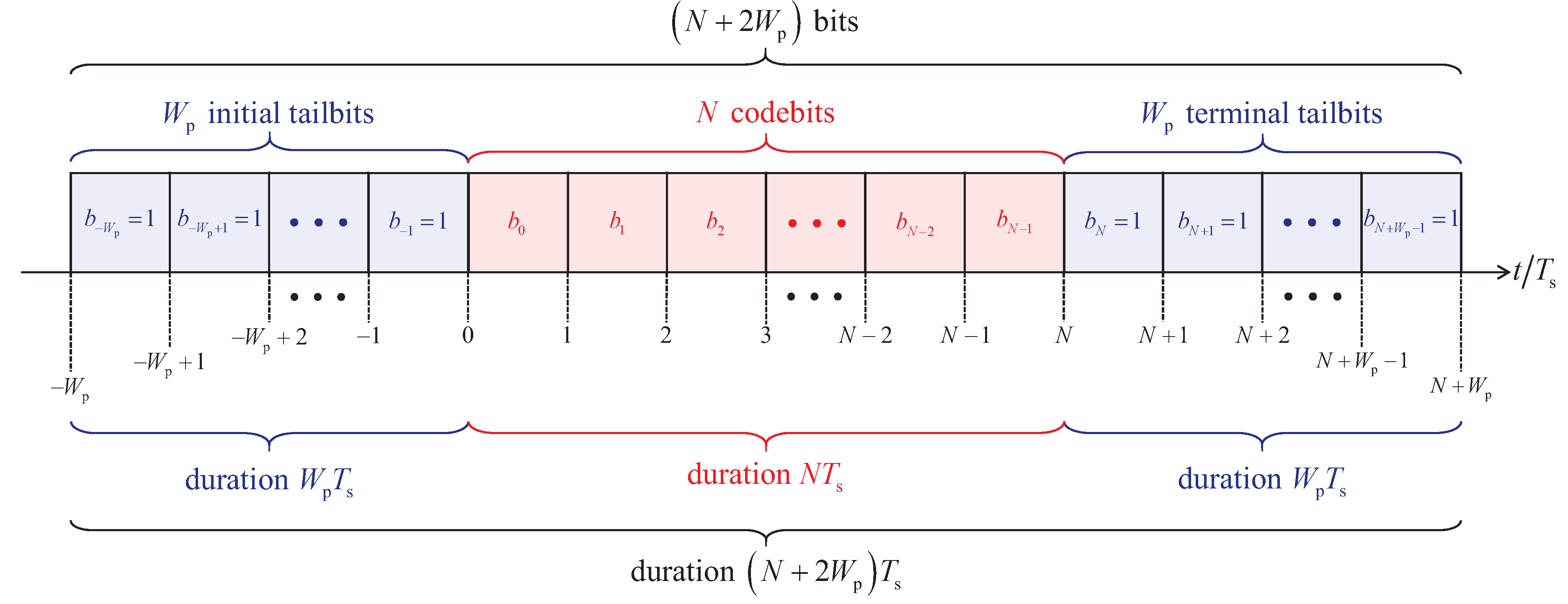
The schematic representation of the transmitted bit vector used when applying the trellis based quantum data detectors, which set out from the Mealy modelling of the FSM representing the multipath quantum channel, is depicted in Figure 3. As pointed out above, the said transmitted bit vector consists of N codebits, initial tailbits and terminal tailbits, hence, containing bits.
Figure 3.
Schematic representation of the transmitted bit vector used when applying the trellis based quantum data detectors, which set out from the Mealy modelling of the FSM representing the multipath quantum channel; the transmitted bit vector consists of N codebits, initial tailbits and terminal tailbits, hence, containing bits.
At the output of the quantum channel, the radiation field resulting from laser emission is linearly superimposed with the omnipresent thermal background radiation field, which is in a thermal state characterized by Bose-Einstein distributed thermal noise photons. As already mentioned above, denotes the average number of thermal noise photons and represents the complex amplitudes of the associated coherent states present in the thermal field. The said linear superposition is modelled by the map
Given
where is a zero phase angle, the corresponding statistical operator in Glauber’s “P-representation” with defined as [9, eqs. (4.6) and (4.10), pp. 134f.]
is denoted by
during the observation time interval , .
Since the function of (24) used in (25) is always nonnegative, the associated laser light is often referred to as “classical.” In contrast, light, for which takes on negative values in some regions is sometimes labelled “nonclassical” [29][p. 60]. However, this distinction may be misleading. For instance, a Fock state is entirely nonclassical by nature [29][p. 58], and, fundamentally, all states of light are governed by quantum mechanics [29][pp. 60, 150]. Thus, the binary classification of light as either “classical” or “nonclassical” may not be entirely appropriate. Considering that Max Planck’s treatment of thermal radiation on December 14, 1900, marked the beginning of quantum mechanics, cf. e.g. [30][pp. 217, 277], and that laser light was theoretically introduced by Albert Einstein in 1917 on the basis of quantum principles, it seems inconsistent not to regard both thermal radiation and laser light as “nonclassical”.
With the regular Laguerre polynomial of degree , we find
neglecting any phase coherence, see also [19][p. 2], [9][pp. 136f.]. Equation (26) is based on the assumption that the quantum receiver front-end essentially consists of a photon counting detector. This photon counting detector measures the number of photons present at the receiver during the observation time interval [19]. Using the trace operation, denoted by , and the projection operator defined as ,
is the conditional probability of detecting photons at the photon counting detector, given the transmission of the codeword . Equation (27) describes this probability as a Laguerre distribution, see also [5, eq. (4.71), p. 174]. Notably, coincides with the transition probability associated with the FSM introduced earlier [19]. It follows that equation (27) assumes the use of an ideal photon counting detector, such as the one discussed in [31][pp. 231f.], as the front-end component of the optimum quantum data detection scheme.
If the photon counting detector cannot precisely count the exact number of photons but is only able to differentiate among zero photons, one photon, or more than one photon, we may use , and equal to instead of for arbitrary [19]. Accounting for real-world effects such as dark counts with the mathematical expectation and quantum efficiency , in equation (27) should be replaced by and has to be replaced by [19].
Based on the above discussion, the actual number of received signal photons in the ith observation time interval results from a linear superposition of Poisson distributed random variables , each with mean . Consequently, itself follows a Poisson distribution [19,32]. It is important to note that Poisson distributed random variables are, by definition, mutually independent [32]. Moreover, the thermal noise photons, governed by the Bose-Einstein distribution, follow a memoryless geometric distribution [19,32]. As a result, measurements taken across any two disjoint observation time intervals are statistically independent. This insight aligns with Forney’s classical considerations [28].
With reference to, e.g., [33][pp. 100-104], the likelihood function , which denotes the conditional probability of observing the photon count vector
given the transmission of the codeword including the terminal tailbits, is defined as follows. Let represent the tensor product of the corresponding statistical operators , and the tensor product of the associated projection measurement operators . Then, the likelihood function is given by:
This expression reflects the joint probability of measuring the specific photon count sequence conditioned on the transmission of the bit sequence , via the tensor product structure of the quantum states and measurements across all observation intervals. We obtain
When the codebits are treated as outcomes of statistically independent random experiments, the a-priori probability of a specific codeword including the fixed-value terminal tailbits set to 1 is given by the regular product of the individual a-priori probabilities
Applying the definition of conditional probability as found in [Def. 3.25, p. 270 [17], the corresponding a-posteriori probability is obtained by
where denotes the total probability of observing the photon count vector , accounting for all possible codewords. Using the definition of the conditional probability [17,Def. 3.25, p. 270], [34, eq.
(5), p. 5], we yield
from (30) after multiplying by the joint a-priori probability of (31).
The likelihood function and its logarithmic counterpart
as well as the a-posteriori probability , or its logarithmic form
constitute the foundation of the quantum data detection process that directly follows photon counting and serves to mitigate ISI [19]. The term is referred to as the metric increment. In summary, optimum quantum data detection leverages either the likelihood function , as defined in (30), or the a-posteriori probability , see (33). Since classical channel decoding follows the quantum detection step, cf. Figure 1, producing LLRs at the quantum data detector output, assembled into the LLR vector , is advantageous.
Referring to optimum quantum data detection as first presented in e.g. [19,20,21], like in Section 2.3, we set out from the ith observation time interval . Again, with the Kronecker symbol , with the cost equal to of the decision in favor of hypothesis when the codebit with value m was transmitted, , and with the Hermitian measurement operator reflecting the hypothesis , in the case of the MAP concept [17, eq. (3.1181), p. 433] the average cost of the observational strategy in the said ith observation time interval is
which is a modified version of (36), replacing used in (36) by , hence taking the FSM related to the ISI into account explicitly.
Each is diagonal in the Fock basis, with the Fock state vectors acting as eigenkets, and the associated eigenvalues given by , which are equal to . As an example, consider the Hermitian detection operator in equation (36), corresponding to and given by
with the eigenvalues
Accordingly, the optimum measurement operators that minimize of (36) and are naturally realized by the ideal photon counter discussed in Section 2 are given by and given by [9].
At the conclusion of the measurement within the ith observation time interval , the exact Fock state of the received radiation field, as present in the ideal photon counter, is known. Consequently, only the projector within or contributes a nonzero eigenvalue . This nonzero eigenvalue is then evaluated using the conventional classical likelihood ratio test. Nonetheless, due to the presence of ISI, the decision made in the ith observation time interval not only depends on earlier transmitted codebits but also influences the decisions in following intervals. As a result, and as reflected in equation (33), the classical likelihood ratio test must be modified, accordingly, taking the following form
This result is an extended variant of Helstrom’s theory [9], as expressed in equation (33). Hence, the optimum MAP symbol by symbol quantum data detection strategy is expressed as
cf. e.g. [35][p. 216], being a classical likelihood ratio test, because we left the quantum regime at the end of the quantum measurement process. However, due to the occurrence of ISI, modelled by the FSM discussed above and, thus, by a Markov chain, (40) requires an appropriate detection scheme, e.g. the trellis based Bahl-Cocke-Jelinek-Raviv (BCJR) algorithm [17,19,35,36]. It seems that this approach has been first introduced by [19].
Correspondingly, also taking ISI and Markov chain modelling into account explicitly, with (33), the optimum MAP sequence quantum data detection strategy is presented by
cf. e.g. [35][p. 216], which can be implemented by the trellis based Viterbi algorithm [17,19,35].
Maximizing the likelihood function over all possibly transmitted codewords will yield the maximum-likelihood (ML) sequence detector, which can be realized by the soft output Viterbi algorithm (SOVA) [17,19,35]. Maximizing the a-posteriori probability over all possibly transmitted codewords will yield the MAP sequence detector. Since a-priori information is processed in the latter case, the corresponding variant of the SOVA is termed APRI-SOVA [35,37]. Both the SOVA and the APRI-SOVA are considered optimum because they maximize the probability of correct sequence detection, which is equivalent to minimizing the sequence error probability, provided that the metric increments discussed above are used. Details of the mode of operation of the SOVA and the APRI-SOVA have been well-known [17,19,28,35,37].
ML symbol by symbol detection focuses on maximizing the conditional probabilities of the observed data given the symbol, , while MAP symbol by symbol detection aims to maximize the posterior probabilities of the symbol given the observed data, [17,35]. To reduce computational complexity, both detection methods are typically implemented in the log domain, similar to optimum sequence detection. Accordingly, ML symbol by symbol detection employs metric increments , whereas MAP symbol by symbol detection uses metric increments of the form [17,19]. Both approaches can be efficiently realized using the BCJR algorithm [17,19,36], which is considered optimum as it maximizes the probability of correct symbol detection, equivalently, minimizing symbol error probability, when the metric increments are used. The operational details of the BCJR algorithm are well-established, see e.g. [17,36]. It is important to note that optimum symbol by symbol detection schemes implemented in the log domain apply the Jacobian logarithm [17][pp. 472f.], which leads to the so-called “log-ML” and “log-MAP” algorithms [17][p. 479]. Approximations of the Jacobian logarithm yield variants known as “max*-log-ML” and “max*-log-MAP”, as well as “max-log-ML” and “max-log-MAP”, respectively [17][pp. 472f., p. 479].
Optimum sequence quantum data detectors, as well as optimum symbol by symbol quantum data detectors, operate as “forward/backward” algorithms that conceptually consist of four key processing units. These are:
- 1.
- The transition metric unit, which computes the metric increments for ML detection, or for MAP detection.
- 2.
- The forward recursion unit, responsible for calculating the forward path metrics.
- 3.
- The backward recursion unit, which either computes the backward path metrics or performs traceback to identify the most likely path through the trellis.
- 4.
- The LLR generation unit, which produces the LLR vector mentioned earlier.
Importantly, only the computations within the transition metric unit differ from those in e.g. classical mobile radio, such as mobile radio detection. The other three units can be reused without modification.
For the SOVA and the APRI-SOVA algorithms, only approximate LLRs can be generated, using three distinct LLR computation methods known as the “SIMPLE RULE (SR)”, the “HUBER RULE (HR)”, and the “BATTAIL RULE (BR)” [17][pp. 463-475]. In contrast, all optimum symbol by symbol quantum data detectors produce LLR vectors containing exact LLRs when implemented as log-ML or log-MAP algorithms, and approximate, though very close to exact, LLRs in the cases of max*-log-ML, the max*-log-MAP, the max-log-ML and the max-log-MAP. implementations.
Trellis based reduced state quantum data detection sets out from the now well-known trellis based optimum sequence quantum data detection, respectively the trellis based optimum symbol by symbol quantum data detection discussed above. Like in the cases of these optimum data detection schemes, the reduced state quantum data detection continues until all LLRs to be determined and, consequently, all the corresponding data symbols have been detected. Trellis based reduced state quantum data detection requires small modifications and extensions of the transition metric unit and the forward recursion unit, which we will discuss in what follows. Since the said modifications and extensions only concern the transition metric unit and the forward recursion unit, which are identical in the case of the max-log-MAP symbol by symbol detection and the SOVA, the novelties presented are identically applicable to
- the trellis based reduced state sequence quantum data detection, which is formed by setting out from the SOVA, termed rsSOVA with the “prefix rs” indicating the reduced state version, respectively from the APRI-SOVA, termed rsAPRI-SOVA, and
- the trellis based reduced state symbol by symbol quantum data detection, which is formed by setting out from the max-log-MAP symbol by symbol detection, termed rsmax-log-MAP, the max-log-ML symbol by symbol detection, termed rsmax-log-ML, the max*>-log-MAP symbol by symbol detection, termed rsmax*-log-MAP, the max*-log-ML symbol by symbol detection, termed rsmax*-log-ML, the log-MAP symbol by symbol detection, termed rslog-MAP and the log-ML symbol by symbol detection, termed rslog-ML, the latter two differing from the max*-log-ML symbol by symbol detection and the max-log-MAP symbol by symbol detection only in the used version of Jacobi’s logarithm but not in the processing of the trellis states and the trellis transitions.
Suppose that we require reduced state quantum data detection with only trellis states, , , . Using explicitly, (21) can be written as follows
Reduced state data detection requires that the binary data symbols , ⋯, contained in the third term on the right side of (42) are known to the quantum data detector prior to the trellis transitions . This requirement calls for preliminary decisions , ⋯, needed for the transition metric computation and hence in the forward recursion. The said preliminary decisions can be accomplished by recursive processing and adds iteratively one single decision per forward recursion step. Therefore, reduced state quantum data detection requires the modification of the transition metrics computation by using of (42), which relies on the preliminary decided binary data symbols , ⋯, and the extension of the forward recursion by adding preliminary decision taking.
In the reduced state trellis, there are trellis transitions , which originate at those states
leading to the possible forward recursion path metrics
denoting the path metric of the state at the time instant i. Also, there are trellis transitions , which originate at those states
leading to the possible forward recursion path metrics
,
denoting the path metric of the state at the time instant i.
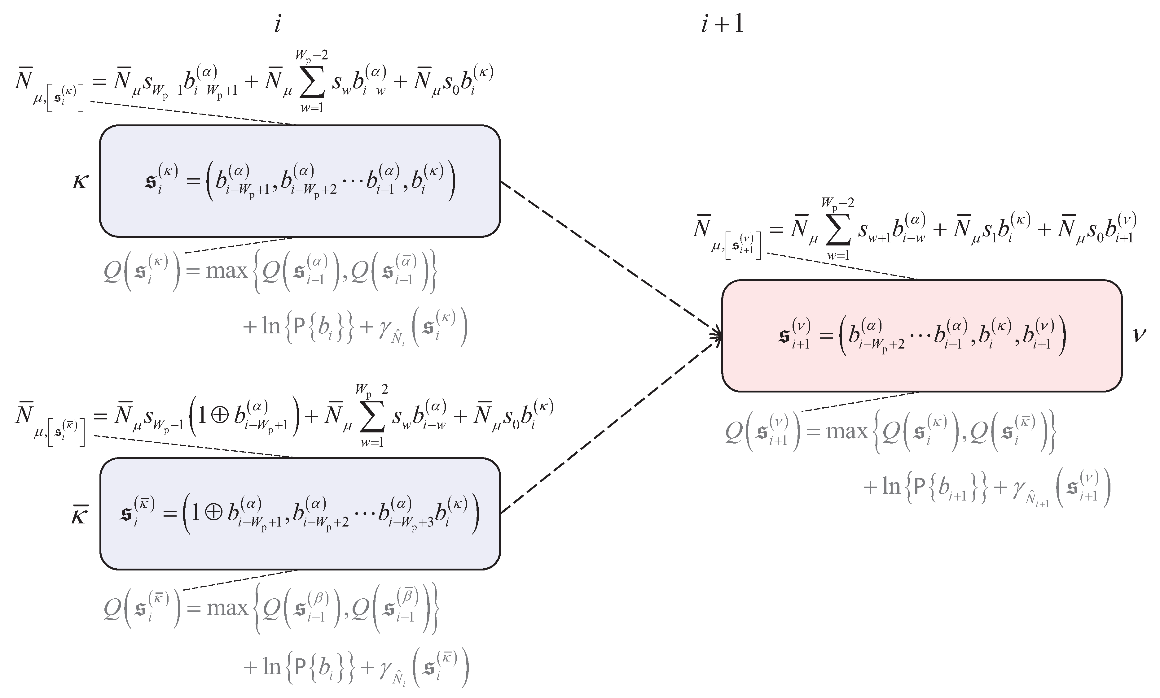
Figure 4 depicts a butterfly of the trellis with states per time instant, considered in trellis based reduced state quantum data detection, which comprises of the two states of (43) and of (44) at the time instant i and the two states equal to and equal to at the time instant . The butterfly consists of two transitions originating at the state at time instant i and two transitions originating at the state at time instant i. Two of these four transitions terminate at the state equal to at time instant and the remaining two of these four transitions terminate at the state equal to at time instant .
Figure 4.
Butterfly of the trellis with states per time instant considered in trellis based reduced state quantum data detection; on-off keying (OOK) is assumed.
Figure 4.
Butterfly of the trellis with states per time instant considered in trellis based reduced state quantum data detection; on-off keying (OOK) is assumed.
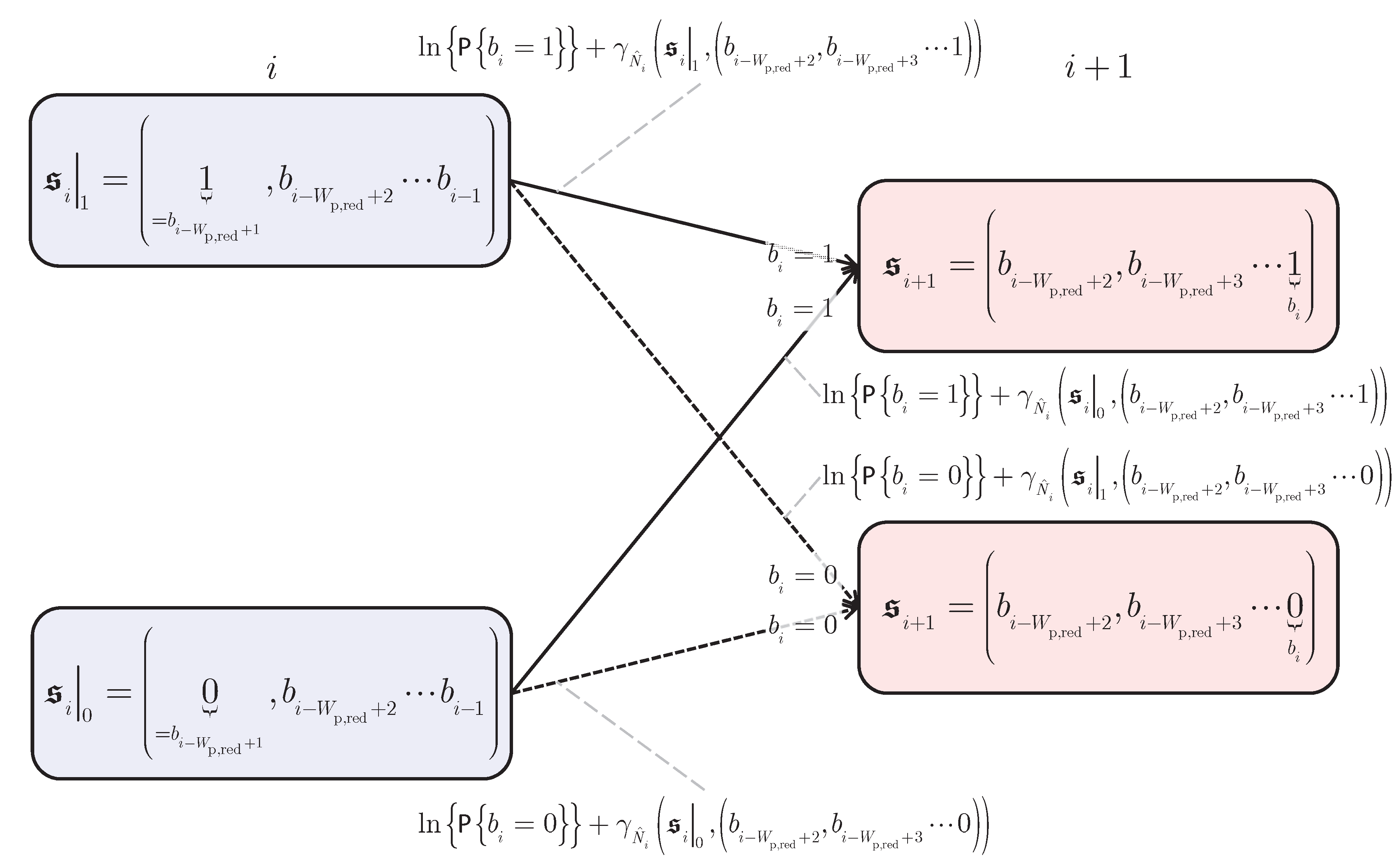
When summing up all the above-mentioned possible forward recursion path metrics by iteratively applying Jacobi’s logarithm, we yield the forward recursion estimate of the logarithmic probability . Next, when summing up all the possible forward recursion path metrics by iteratively applying Jacobi’s logarithm, we yield the forward recursion estimate of the logarithmic probability . Subtracting from yields the forward recursion LLR of , which is to be used for the preliminary decision . Since we now have the viable decision , we may continue with the next iteration step in the forward recursion.
Figure 5.
System design of the Kohonen maps based detector employing a neural network using variable neuron weights, cf. e.g. [22][Fig. 1].
Figure 5.
System design of the Kohonen maps based detector employing a neural network using variable neuron weights, cf. e.g. [22][Fig. 1].
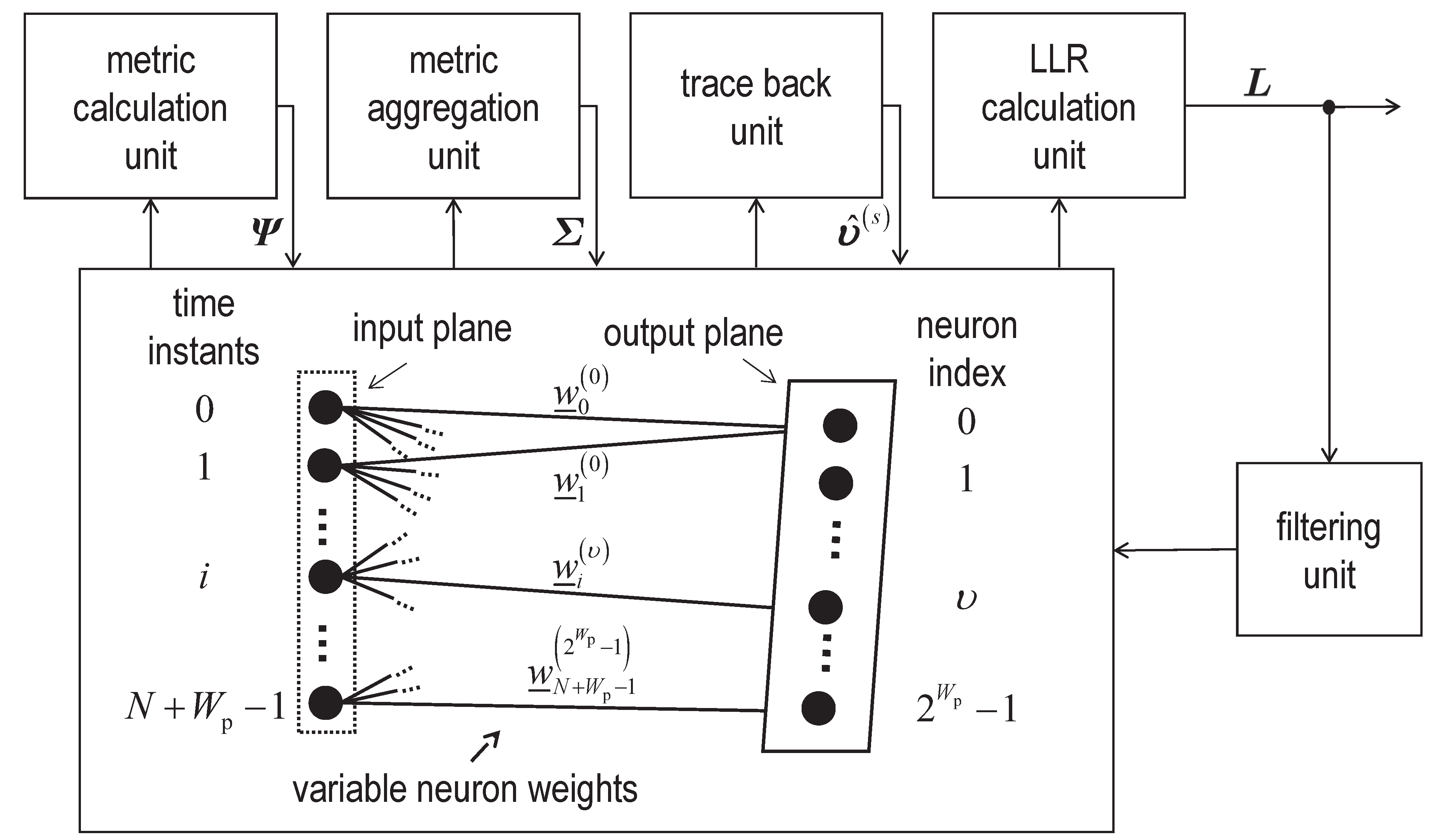
While state reduction is an advantageous strategy for managing detection complexity, Kohonen maps can be employed for resource-efficient implementations, and near optimum performance in classical mobile communication systems [22]. The Kohonen maps based sequence detector, also referred to as “Kohonen maps based detector” or “Kohonen detector”, is also applicable to quantum channels. It consists of four processing units, namely the metric calculation unit, the metric aggregation unit, the trace back unit and the LLR calculation unit [22]. The combination of these four units follows the signal processing principle of a APRI-SOVA by applying a neural network with a one-dimensional linear structure in both the input plane and the output plane using distinct features of the Kohonen map by appropriately adjusting the weights and the distance function [22]. More specifically, the neural network adopted by the Kohonen maps based detector is a hybrid of learning vector quantization (LVQ) and Kohonen maps, both belonging to the family of soft competitive learning clustering algorithms [38]. This approach enables leveraging neural networks to perform near optimum sequence detection by efficiently utilizing existing hardware resources [22]. Training the Kohonen map by incorporating LLR feedback has been shown to improve the overall performance of the Kohonen maps based detector [22].
In order for the Kohonen maps based detector to be applied in quantum communication channels, the aforementioned FSM has to be modelled by means of a Moore machine. In the case of Moore modelling, the FSM contains unique states equal to at each time instant . For this reason, we will use initial and terminal tailbits, setting equal to 1 for all .
The schematic representation of the transmitted bit vector used when applying the Kohonen map based quantum data detector, which sets out from the Moore modelling of the FSM representing the multipath quantum channel, is shown in Figure 6. As pointed out above, the said transmitted bit vector consists of N codebits, initial tailbits and terminal tailbits, hence, containing bits.
Figure 6.
Schematic representation of the transmitted bit vector, used when applying the Kohonen map based quantum data detector, which sets out from the Moore modelling of the FSM representing the multipath quantum channel; the transmitted bit vector consists of N codebits, initial tailbits and terminal tailbits, hence, containing bits.
Each possible state at a given time instant i is associated with a state number, i.e. a state index . Interpreting the FSM as a Moore machine involves a doubling of the number of states and a reinterpretation of the transition metrics, as they no longer depend on transitions, i.e., both the initial states and the target states, but solely on the target states. We further denote the set of possible states in the Mealy case by and the corresponding set in the Moore case by . The remodelling as a Moore machine necessitates the introduction of a mapping function in order to assign the previously determined transition metrics , for the Mealy case to transition metrics for the Moore case , respectively, , . We define a surjective mapping
to assign the transition of a Mealy state pair to a Moore state. For each the mapping is defined as
where denotes the floor function (in German “Gaußklammer”). Furthermore, denotes the state index of the initial state and the state index of the target state in the case of Mealy modelling.
Once the transition metrics according to Moore modelling are obtained and summarized in a matrix , the Kohonen detector operates similarly to the case of classical wireless communication systems. At this stage, the Kohonen map serves as a state mapper allowing for an adequate add-compare-select (ACS) operation for the permissible state transitions [22]. In what follows, denotes a possible predecessor state with its state index at the time instant i of the successor state with state index at the time instant . The output neuron for the state with state number at the time instant is configured with the weight vector
using
where denotes the path metric of the state with state number at the time instant i. Any state can be reached by two distinct predecessors, and say. In order to determine the path metrics at the time instant for each possible successor state , solely the weights of the Kohonen map must be examined. We obtain
which can be arranged in the path metrics row vectors
We will illustrate the above discussions of the soft output Kohonen maps based quantum data detection in what follows. Let the states with the state indices and refer to the predecessor states at time instant of the state with the state index at time instant i. Furthermore, let the state indices and refer to the predecessor states at time instant of the state with the state index at time instant i. As shown in Figure 7, the state
with the state index , , … and denoting the particular bit values associated with this state , and the state
with the state index , , … and denoting the particular bit values associated with the state , are the predecessor states at time instant i of the state
with the state index at time instant . The aforementioned states of (51), of (52) and of (53) are part of the trellis representing the multipath quantum channel with possibly nonvanishing channel coefficients , , setting out from the Moore modelling applied in the soft output Kohonen maps based quantum data detector. In Figure 7, the average numbers
and
of signal photons at the photon counter are associated with the appropriate states. Also, the recursive computation of the path metrics
by the soft output Kohonen map based quantum data detector is also illustrated.
The calculated path metrics are arranged in the matrix
for further processing. The optimum path is found in the trace back unit by again utilizing the Kohonen map as a state mapper, yet in a reverse-oriented manner. The weights of the neurons representing the possible predecessor states are configured with
Denoting the state index of the survivor state at time instant by , its predecessor state is found according to
The remaining predecessor states can be determined recursively. All predecessors along the survivor path can be arranged in the vector of length . Similarly to the case of SOVA, respectively the APRI-SOVA, approximate LLRs can be generated using the Kohonen detector [22].
Owing to its simplicity and promising performance, the authors choose to begin with the aforementioned “SIMPLE RULE” (SR). According to the SR, approximate LLRs are built based on the path metric differences of the survivor and concurrent predecessor states [p. 466 [17, p. 466]. In the case of Moore modelling of the FSM, the path metric difference at time instant is given by
where denotes the path metric of the concurrent predecessor at time instant i. The structure of the Kohonen map employed in the generation of LLRs mirrors that of the trace back unit, with the sole modification being the inversion of the sign of the concurrent predecessor state’s path metric and the insertion of zeros instead of for impermissible state transitions, i.e.
The path metric difference represents the distinct metric deviation that allows to distinguish between whether the FSM was in the predecessor state or in the concurrent predecessor state . Due to the structure of FSM modelling and the influence of ISI, these two states differ by only a single symbol, specifically, the one at time instant . Therefore, the path metric difference is interpreted as a reliability measure for that particular symbol at time instant . The LLRs are found recursively using
The updates according to the “HUBER RULE” (HR) and the “BATTAIL RULE” (BR) can be performed in accordance with [pp. 469, 474 [17, pp. 469, 474].
In order to improve the adaptability of the Kohonen map based detector, a novel updating procedure was also introduced, where, instead of investigating spatial distribution of FSM states, a probability based neighborhood function is calculated [22]. These probabilites are calculated based on the LLRs, which can be filtered and fed back in order to update the Kohonen map. Since Kohonen maps follow a “winner takes most” approach, not only the weights of the winning output neuron are updated, but also those within a defined “winning neighborhood” . The probability of each state at each time instant is governed by the a-priori probabilities of the most recently received codebits, which are supposed to be mutually independent. It is thus obtained by
Given the state probability (66) and the probability threshold , which must be exceeded if the weights of a neuron shall be updated, the neighborhood of the winning output neuron is given by
[22]. This purely local perspective can be improved by using a “forward/backward” approach to obtain the optimum state probabilities.
By combining two megatrends, namely artificial intelligence and quantum communications, soft output quantum data detectors using Kohonen maps may provide low-complexity, high-performance detection methods that enhance the scalability and efficiency of next-generation communication networks.
Figure 7.
Schematic representation of the connections between the states and with the state indices and at the time instant i with the state with the state index at the time instant , which are part of the trellis representing the multipath quantum channel with possibly nonvanishing channel coefficients , , setting out from the Moore modelling applied in the soft output Kohonen maps based quantum data detector; the average numbers , and of signal photons at the photon counter are associated with the appropriate states; also, the recursive computation of the path metrics , and by the soft output Kohonen map based quantum data detector is also illustrated.
3. Polar Coding for Wireless Quantum Optical Transmission
3.1. General Concept of Polar Codes
In 2009, Erdal Arikan introduced polar codes as a class of capacity-achieving error-correcting codes for binary memoryless symmetric channels [39]. The construction of polar codes is inspired by Reed-Muller codes and builds on the Plotkin construction proposed in 1960 [40], or alternatively, it can be described using a recursive formulation based on the Kronecker product [39].
Polar codes are notable for their deterministic construction and their ability to asymptotically achieve the capacity of binary memoryless symmetric channels under successive cancellation decoding. Understanding the polarization process requires some familiarity with information-theoretic concepts such as mutual information and entropy. For a more detailed theoretical background, the reader is referred to relevant literature, cf. e.g. [8, Chapter 4, pp. 336-388]. The key idea of channel polarization is the transformation of a set of identical channels into a set of virtual channels with split reliability levels, which allows a distinction between information bits and frozen bits.
For the construction of polar codes of even length
denotes the input vector to the encoder, containing information bits, and denotes the encoded codeword at the output of the encoder, consisting of the K information bits and the frozen bits. Let be the generator matrix. The polar code is then given by the linear transformation of using [39]
Setting out from the smallest code length, i.e. N equal to 2, the basic generator matrix becomes [41]
being capable of generating both parity and systematic codebits. The square generator matrix of the 3GPP polar code is recursively defined by the multiple Kronecker product [8, Sect. 1.16, pp.
224-233]
Arikan prefers to define the generator matrix in his work based on a permutation matrix, denoted here as , and the identity matrices and [8,39]
The two variants of the linear transformation using , as defined by 3GPP and by Arikan, each require a dedicated decoder structure to correctly decode the encoded message. For N equal to 4, Figure 8 illustrates the decoding scheme according to the 3GPP standard and Figure 9 shows the decoding structure according to Arikan.
Figure 8.
Illustration of the information flow in a successive cancellation decoder based on Arikan’s original construction for a polar code of length .
Figure 8.
Illustration of the information flow in a successive cancellation decoder based on Arikan’s original construction for a polar code of length .
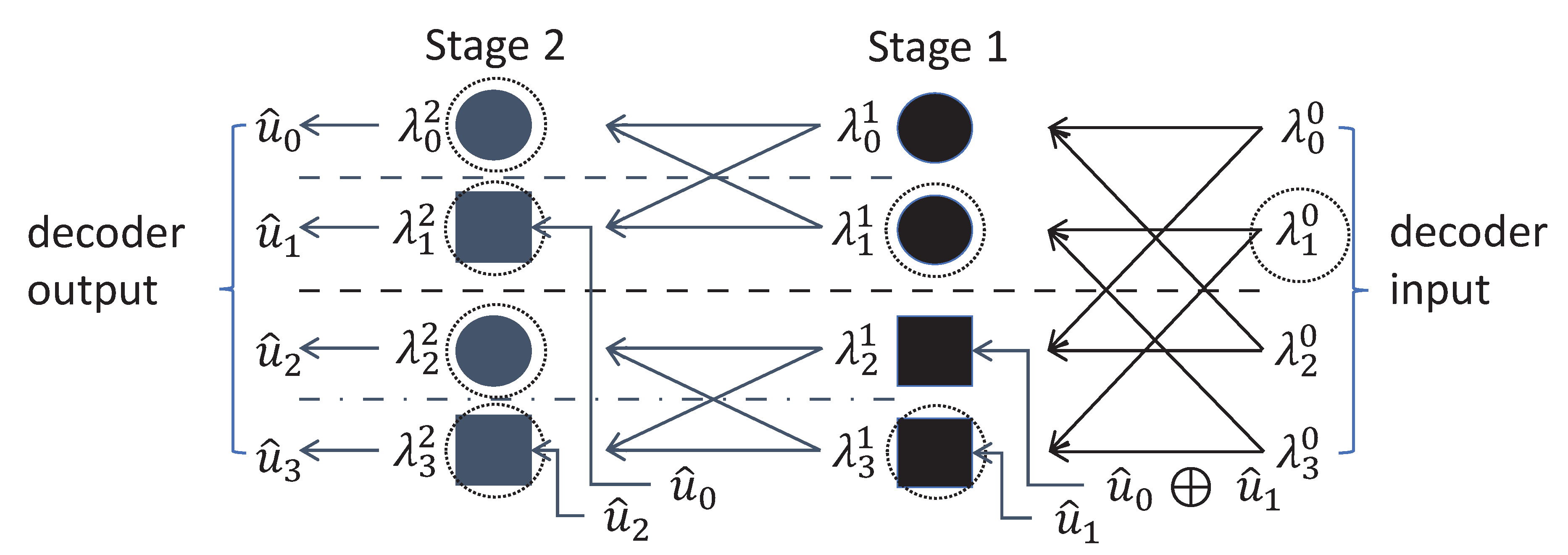
Figure 9.
Illustration of the information flow in a successive cancellation decoder based on Arikan’s original
construction for a polar code of length .
Figure 9.
Illustration of the information flow in a successive cancellation decoder based on Arikan’s original
construction for a polar code of length .
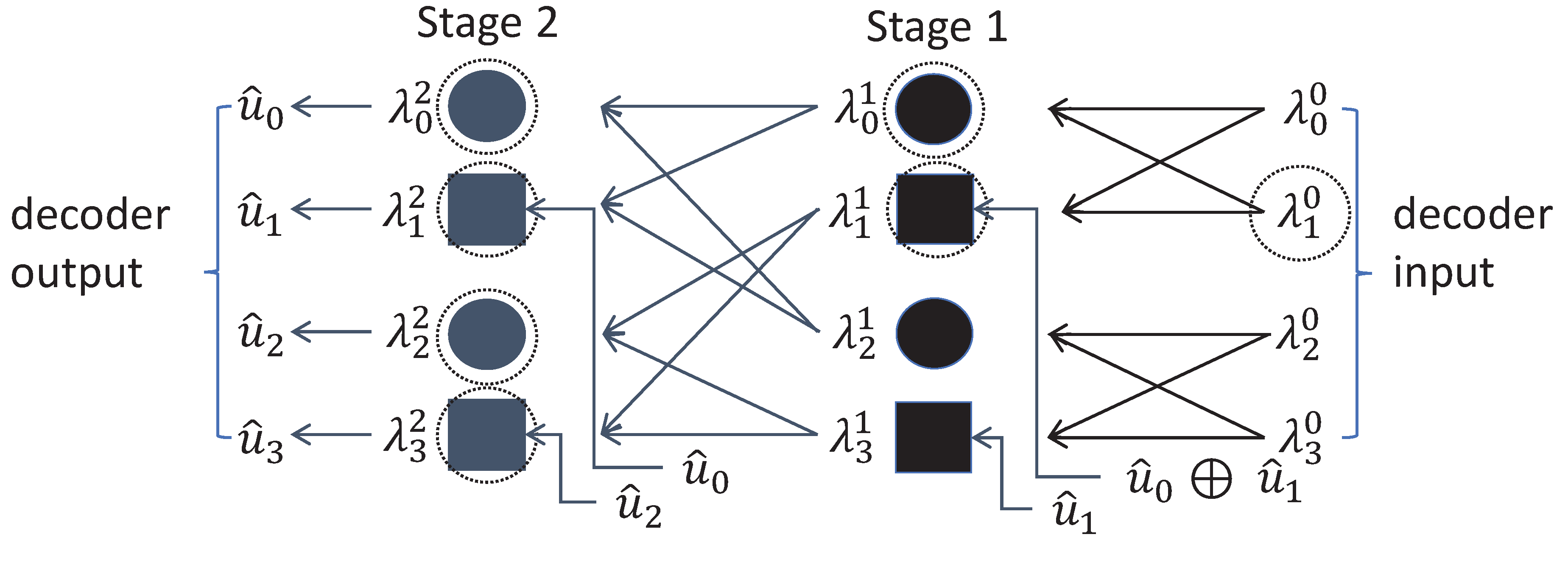
The values represent the LLRs. In each decoding stage, two functions are applied, namely, the f function, represented by circles in Figure 8, and the g function, represented by squares in Figure 8. These functions are used to recursively update the LLRs based on previously decoded bits. The f and g functions operate on two input LLR values, typically denoted as and , and in the case of the g function, also on previously decoded bits . These inputs correspond to values from nodes in the decoding tree. The f and g functions can be defined as follows [8, Eq. (3.114), p. 364; Eqs. (4.260) and (4.261), p. 386]:
The expression for the f function represents an approximation of the exact soft decoding rules using the arctanh [8, Eq. (4.260), p. 386]. After a total of stages, the message is fully decoded using recursive decoding. This process starts with the least significant bit and proceeds toward the most significant bit . Previously decoded bits are reused as intermediate results across the decoding stages.
A comparison of the 3GPP and the Arikan constructions of the polar code reveals that the indexing must be handled differently in the implementation of the respective decoder structures. This is due to the fact that the generator matrices used in the 3GPP and Arikan constructions are not identical and transform the message in different ways through linear operations. Another key difference between the 3GPP and the Arikan constructions lies in the structural symmetry present in every stage in the 3GPP decoder, as indicated by the horizontal dashed lines in Figure 8, which is not present in the Arikan construction. Furthermore, it becomes evident that a decoding error, e.g. at the position of , highlighted as dashed circles in Figure 8 and Figure 9, effects the decoding process differently in each structure. The error propagation paths diverge between the two constructions, as illustrated by the dashed circled elements in the figures. Even under identical channel conditions, the decoders may produce similar but not identical results.
3.2. Design of Polar Codes: Finding the Polar Sequence
Even though the generator matrices are known, constructing the strongest possible polar code for a given code rate equal to remains a laborious task. It requires identifying those virtual channels that should be frozen and thus excluded from carrying information [8,39]. This identification leads to a ranking list of all virtual channels, often referred to as the reliability sequence [8][pp. 347, 364, 378, 380], polar sequence [41], or reliability order [42]. The process of constructing this polar sequence is commonly known as polar code definition [39] or polar code construction [42].
For a combined channel of length N, the process of channel combining and splitting results in a set of polarized subchannels [8, Chapter 4, pp. 336-388]. The task of polar code construction is to select the most reliable subchannels from this set, i.e., to determine an appropriate subset of virtual channels that will be used to carry the information bits. As Arikan has shown in his original work, the polar sequence depends on the transmission channel. For the binary erasure channel, he suggested the Bhattacharyya parameter to determine the polar sequence [39]. Since the Bhattacharyya parameter of a binary erasure channel is equal to the erasure probability , the channel capacity C of a virtual channel approaches 1 when approaches 0 [8].
Arikan’s Bhattacharyya parameter based approach is clearly dependent on the particular channel and its actual quality. Regrettably, it does not seem that the Bhattacharyya parameter can be determined in analytic closed form for the quantum channels considered here. Therefore, other methods for determining the polar sequence when considering transmission channels other than the binary erasure channel must be used such as the Monte Carlo simulation approach [39] and the density evolution method [43]. In all these cases, the definition of the polar sequence will involve lengthy and cumbersome analyses and is likely not to yield a single optimum polar sequence for all circumstances.
The likelihood of never being able to define the optimum polar sequence in a closed form analytic expression and thus at the lowest possible cost has led to the abandonment of the strict requirement for an optimum solution. Instead, the focus has shifted toward a sufficiently good, best possible solution for the time being. In the case of 5G/New Radio (5G/NR), 3GPP delegates have succeded in defining such a polar sequence [41][Table 5.3.1.2-1, pp. 17-19], which enables an impressively low block error ratio (BLER) performance in all required cases. The approach chosen in the 3GPP standardization of 5G/NR sets out from a closed form expression, which to the best of the authors’ knowledge was first suggested in the technical document R1-167209 presented at the TSG RAN WG1 Meeting #86. We will briefly summarize this approach in what follows:
- 1)
- Set out from the virtual channel with index being a nonnegative integer and having the binary representation given by the values beginning from the least significant bit j equal to 0, i.e.
- 2)
-
Then, by replacing 2 by being approximately equal to in (75), define the quality factors called polar weights [42, Eq. (4), p. 2]Comparing (75) with (76), we immediately realize that (76) represents the generalization of the binary representation of (75).
- 3)
- Since a virtual channel with high quality is associated with a large value of the polar weight given by (76), establish the polar sequence as that particular sequence of the indices of in ascending order of the polar weights .
The authors believe that the suggested approach of the technical document R1-167209 presented at the TSG RAN WG1 Meeting #86 presents a promising start. However, owing to the considerable difference between the mobile radio channel and the quantum channel faced in the case of wireless quantum optical communications, it must be studied whether there may exist better polar sequences for wireless quantum optical communications than the existing 3GPP 5G/NR polar sequence published in [41][Table 5.3.1.2-1, pp. 17-19]. In a first step, we will replace (76) by the following definition
of the quality of the virtual channel with index i. The base p chosen in (77) determines the polar weights of the N virtual channels. Nota bene that the representation of (77) is sometimes attributed to Alfréd Rényi as a number theoretical concept published in 1957. However, its roots are more than half a century older as we will see in a moment.
Equation (77) is based on the p-adic expansion of integers illustrated in [45, p. VI; Eq. (2), pp. 49f.], for a finite number of n equal to terms and only nonnegative exponents , a concept well-known in number theory first introduced in 1897 by the German mathematician Kurt Hensel [44], see also [46], yielding a unique result for any nonnegative integer. In the p-adic expansion, the base p is a prime number, however, it is straight-forward and trivial to relax this requirement in favor of any base (in German “Grundzahl”) g[45, p. VI], such as e.g. g equal to 10, leading to the more general g-adic expansion [45, Eq. (7), p. 54]. In the case of the p-adic as well as the g-adic expansions, the coefficients are taken modulo p, respectively, g [45, p. 54]. Hensel also investigated the case of the general base g being a power of the prime number p [45, p. 73]. Setting out from these insights, it is an immediate approach to obtain (77), neglecting the number theoretic burden of this step. Supposing p to be a general, preferrably nonnegative, real number, the said p-adic expansion based approach (77), although according to the above discussion being suboptimum, is channel independent and provides a solution in analytic closed form.
The definition of the polar sequence by a closed expression of the type shown in (77) is elegant, efficient and implementation-friendly. Setting out from these facts, the authors will present further results on the selection of suitable polar sequences for quantum optical communication systems in what follows, proposing distinct polar sequences for wireless quantum optical communications with carrier phase knowledge versus random carrier phase scenarios as such a distinction facilitates a lowest possible BLER for the considered applications. In other words, the authors suggest using channel adaptive polar sequences in future applications, in particular, for wireless quantum optical communication systems.
In wireless quantum optical communications, the transmission is predominantly governed by unknown, random carrier phase most of the time, cf. e.g. Section 2.3 and [20]. In the absence of any channel state information (CSI) at the transmitters and the receivers, the polar sequences corresponding to
and
are found to be good choices. Furthermore, if the transmission preserves the carrier phase, using (79) leads to the preferable polar sequences for any code rate . These observations show that the suggested base p equal to used in the technical document R1-167209 presented at the TSG RAN WG1 Meeting #86 differs from the choice of p in the case of wireless quantum optical communications. The following Algorithm 1 summarizes the approach.
| Algorithm 1 Computation of Polar Sequences |
Require: Code length N, positive real , e.g. , 2, , ; exponent , e.g. the code rate
|
Since standardized implementations typically prefer a single, channel-independent polar sequence, the authors propose a polar sequence suitable for both coherent and incoherent transmission. This new polar sequence is derived from the combination of the two previously considered polar sequences found for p equal to and . To the best of the authors’ knowledge, the approach of constructing a new polar sequence by combining multiple sequences has not been previously published and therefore seems to be novel in the context of constructing new polar sequences.
This work considers two analytical approaches for combining multiple reliability sequences. The first approach considers, at each position of the polar sequence, only the largest channel index i among the available sequences. Therefore, the largest channel index i at that position is selected as the winner. The second approach evaluates a data set consisting of at least three predefined reliability sequences. In this case, the selection is based on the absolute frequency of each channel index i at the position . If no clear winner can be determined on the basis of frequency, the decision falls back to the selection of the larger channel index i according to Algorithm 1. In this manuscript, the first approach is preferred as it is more resource-efficient and easier to implement. The procedure to generate the aforementioned combined polar sequence is summarized in the novel Algorithm 2. The central idea of this algorithm is to resolve conflicts incrementally, position by position, by giving preference to the channel with the higher channel index i and filling the remaining gaps with unused indices, sorted by ascending weight. It is almost needless to mention that the iterative application of Algorithm 2 will facilitate to combine a multitude of available polar sequences.
| Algorithm 2 Combination of Two Polar Sequences |
|
Require: Two polar sequences , , each of length N Ensure: Combined polar sequence of length N
|
3.3. Turbo Equalization with Polar Codes
Turbo equalization is an iterative scheme, which involves both data detection and channel decoding, striving for the iterative reduction of errors contained in the decoded message . Turbo equalization was first introduced in 1995 [47] in the case of additive white Gaussian noise (AWGN) channels with ISI and with as well as without fading. Both the data detector and the channel decoder applied in [47] were using the SOVA. A similar concept for source-controlled channel decoding was used in [37,48], which clearly demonstrates the necessity of providing soft information like LLRs from the source decoder to the channel decoder. None of these concept has yet been applied to polar coded wireless quantum optical communications via multipath quantum channels with uncorrelated scattering and ISI.
The principle of turbo equalization in polar coded wireless quantum optical communications via multipath channels with uncorrelated scattering and ISI is depicted in Figure 10. The generic receiver consists of the quantum data detector, the polar code decoder, the block error iteration control unit and the extrinsic information computer. Since in wireless communication systems interleaving is widely deployed and since the authors suggest the inclusion of quantum optics in future wireless communication systems, the optional introduction of an interleaver with the interleaver (permutation) matrix Π and its corresponding deinterleaver with the matrix is also depicted in Figure 10. In this work, a simple square block interleaver will be considered when analyzing turbo equalization for wireless quantum optical communications. Suppose the square interleaver matrix , yielding the interleaver size . Using the ceiling function (in German “obere Gaußklammer”) , choose equal to and form the extended codeword
of length . The said extended codeword of (80) is then entered into the square block interleaver from left to right in a row by row fashion, beginning with the first row and the first column and the interleaved extended codeword is determined from top to bottom in a column by column fashion, beginning with the first row and the first, i.e. leftmost, column. The deinterleaving is accomplished by the reversed operation.
Figure 10.
Generic receiver structure for data transmission in polar coded wireless quantum optical communications via multipath channels with uncorrelated scattering and intersymbol interference (ISI) including the turbo equalization concept.
Figure 10.
Generic receiver structure for data transmission in polar coded wireless quantum optical communications via multipath channels with uncorrelated scattering and intersymbol interference (ISI) including the turbo equalization concept.
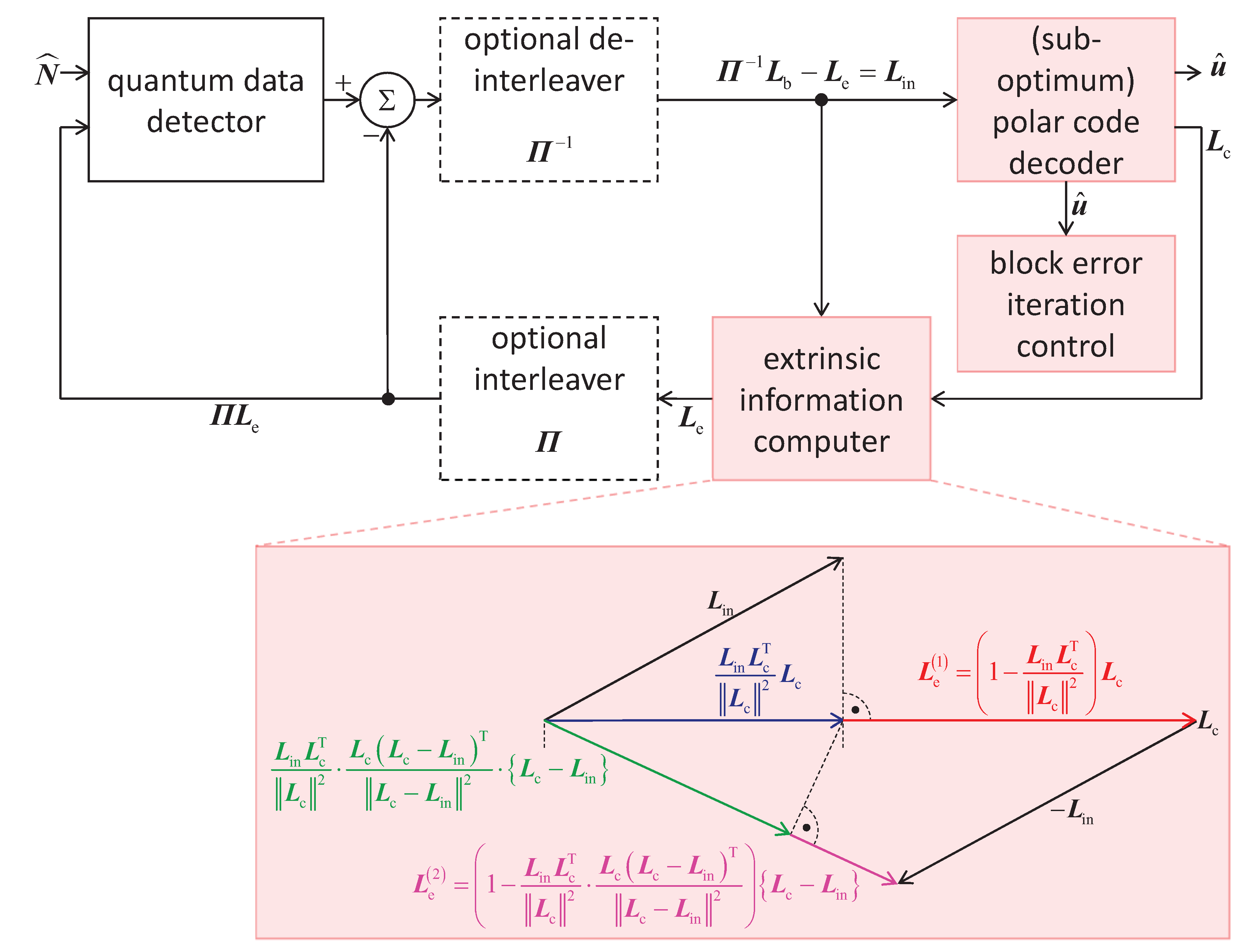
Turbo equalization is only possible when the quantum data detector is capable of processing a-priori information. Regrettably, the said a-priori information is not known to the receiver prior to the quantum data detection. This fact requires the generation and continuous updating of some sort of information, which can serve as “a-priori information”, while the turbo equalization iterations are ongoing. Hence, there is no true a-priori information but some sort of an estimate. This estimate must be delivered by some receiver unit, which cannot be located in front of the input of the quantum data detector due to the above-mentioned prerequisite. In fact, a modified channel decoder, which in addition to providing the decoded message is capable of determining the soft output vector corresponding to the , codebits , , provides the basis for the said estimate of the aforementioned “a-priori information”, which we will call the interleaved extrinsic soft output vector denoted by . In the context of the turbo equalization considered here, the expression “extrinsic” means “generated during the channel decoding in addition to the input vector ”. In other words, the extrinsic soft output vector has not been part of the input to the channel decoder prior to the channel decoding.
According to Figure 10, after processsing the photon count vector introduced in (28) and the “a-priori information” , the quantum data detector delivers the soft output vector corresponding to the , codebits , . In order to optimize the mutual information governing the turbo equalization process just as in the case of turbo code decoding, the “a-priori information” is subtracted from prior to the optional deinterleaving. At the output of the deinterleaver, the input vector
prevails, which is obtained from e.g. (88) for equal to 1 and represents the input to the polar code decoder. Besides the decoded message , the polar code decoder generates the vector , which is composed of soft outputs associated with the , codebits , . In the block error iteration control unit, the decoded message is analyzed in order to identify block errors. If a block error is detected by e.g. evaluating a cyclic redundancy check (CRC) code, which is supposed to be part of and, consequently, of , according to the 5G/NR specification [Sect. 6.13.2.1, pp. 140-142 [49], a further turbo equalization iteration is carried out. In the case successfully passes the analysis in the block error iteration control unit without any detected block error, the turbo equalization is terminated for the inspected message . As illustrated, the authors deploy adapative iteration control of the turbo equalization, which facilitates considerable savings of processing efforts and, consequently, power consumption.
In the case of a required turbo equalization iteration, the soft output vector is processed in the extrinsic information computer, generating the extrinsic soft output vector at its output by exploiting the input vector of (81). After the optional interleaving, which yields , the quantum data detection process can start again.
The success of turbo equalization based on polar coding relies on two prerequisites, namely
- 1)
- the availability of soft information per codebit , collected in the soft output vector and
- 2)
- the availability of extrinsic information of good quality, collected in the extrinsic soft output vector .
With respect to the first item, two alternative approaches have been mentioned in the open literature. The first concept is based on the sum product algorithm (SPA) [8, Sect. 3.2.3, pp. 332-335] used for the decoding of LDPC (low density parity check) codes when computing the LLRs of the check nodes, cf. e.g. [8, Sect. 3.2.2, pp. 327-332]. The second concept was suggested by Fayyaz and Barry as part of their soft cancellation (SCAN) polar decoding scheme [50]. Since the first concept provides correct LLRs, the authors do not pursue the second approach [50] further in this manuscript.
Nota bene that, although claimed, [50] does not provide any turbo equalization. It is merely a clever adaptation of the SPA to polar codes.
Furthermore, the rather little performance improvement of the SCAN polar code decoding reported by Fayyaz and Barry [50] demonstrates the strong correlation of the soft inputs vectors and the corresponding soft output vectors of the SCAN polar code decoder, which is governed by the code structure.
Regrettably, it seems that no one has explicitly stated the chosen approach in the context of polar codes. Hence, the authors are now making up for this omission in what follows:
Suppose that in the nth, , column of the generator matrix of the polar code of length N only the elements in the rows denoted by with taken from a subset of are equal to one.
Let us denote the said subset by , having the cardinal number .
Define
Denoting the soft output associated with the Nth message bit by , for every n, initialize by
Denoting the “box plus” operation by ⊞, which realizes
either exactly or by some approximation, cf. e.g. [51][pp. 357-366] and the references given therein, while iterate
The final output is
Probably the most critical part of turbo equalization lies in the determination of the extrinsic soft output vector , cf. the second item mentioned above. According to Douillard’s seminal paper [47, Fig. 5, p. 510], we obtain
Although Douillard et al. do not explicitly give the range of the coefficient , the reference to the variance on page 509 of [47] implicitly suggests that is nonnegative and real. It is also plausible to suppose that (89) implies . In 1997, Hagenauer [52, Fig. 4, p. 7 ] illustrated that (87) is optimum in the case of MAP based symbol by symbol data detection and MAP based channel decoding. A third known approach appeared in 1993 in the seminal paper [53, p. 1096] by Berrou et al. introducing turbo codes for the first time, suggesting the ith component of the extrinsic soft output vector to be
although all constituent decoders applied in [53] are MAP symbol by symbol decoders.
Since optimum polar code decoders, which can be efficiently realized, are not known, the authors suppose that deployed polar code decoders are and will probably always be suboptimum. Therefore, one must raise the question, whether the above-mentioned schemes (87)-(90) are applicable. In what follows this concern will be addressed and the authors will suggest a viable solution for turbo equalization using polar codes.
The treatment of the availability of extrinsic information of good quality, collected in the extrinsic soft output vector , seems still to be in its infancy as far as turbo equalization using polar codes is concerned. In fact, it seems that turbo equalization using polar codes has not been addressed explicitly prior to a paper [54] published in 2024 by Eltohamy, Hofmann, Knopp and Korb. Although not discussed in detail in [54], Eltohamy et al. either use the above stated approach for the generation of the soft output vector or an equivalent one. With respect to the generation of the extrinsic soft output vector , Eltohamy et al. apply [54, Fig. 6, pp. 146f.]
using the real nonnegative scaling factor , which is “empirically optimized”, leaving a certain feeling of discomfort. Surprisingly, may be arbitrarily chosen [54, Fig. 8, p. 147], which suggests a certain degree of novelty in comparison to (87)-(90). Although the number of turbo equalization iterations was not stated in [54], the authors are convinced that this number was fixed in all cases, not being adapative to the actual transmission. Furthermore, the performance gains reported in [54, Figs. 8 and 9, pp. 147f.] seem to be limited. This is a clear hint to the fact that notable correlations between and exist.
Regarding the availability of extrinsic information of good quality, collected in the extrinsic soft output vector , the authors propose the following two realizations of the extrinsic soft output vector, shown as and in Figure 10. The said solutions proposed by the authors present an analytic way forward, avoiding any empirical optimizations. Correlations vanish when the vectors and are mutually orthogonal, at least on average. The demanded orthogonality is however unlikely, which yields a nonvanishing inner product , supposing that and are row vectors and denoting transposition by . Therefore, when subtracting that particular component of , which is collinear to , from , the remainder may serve as extrinsic information of desirable quality. The authors therefore propose the following first version of the extrinsic soft output vector
illustrated by in Figure 10.
The second version of the extrinsic soft output vector, identified by in Figure 10, sets out from the assertion that the extrinsic soft output vector should be collinear with , which has been considered traditionally, cf. e.g. (87)-(90), and is also assumed in (91). As it was already observed by Eltohamy et al. [54], the real nonnegative scaling factor cannot be left equal to 1, hence (87) and its direct descendants do not seem viable. Extending the above derivation leading to (92) yields
cf. the geometrical illustration depicted in Figure 10. With (93), the real nonnegative scaling factor of (91) becomes
Nota bene that both approaches (92) and (93) suggested by the authors are fully adaptive with a clear theoretical foundation and without any empirical optimization. Furthermore, as opposed to the approaches presented in (87)-(91), the novel solutions (92) and (93) suggested by the authors use the real coefficients
- and
- ,
respectively.
4. Selected Simulation Results
4.1. Uncoded Transmission and Reception
First, we will consider the short range transmission via a single path quantum channel, cf. Section 2.3. Consequently, the channel impulse response of the said quantum channel called CIR#1 in what follows has one single nonzero channel coefficient equal to 1, cf. Table 1. Both the scenario without decoherence and, thus, with known carrier phase as well as the scenario subject to decoherence and, hence, with unknown carrier phase, the phase being a uniformly distributed random variable, have been evaluated by simulations in terms of the uncoded bit error ratio (BER) , i.e. the BER obtained before the channel decoding. The obtained uncoded BER curves are depicted in Figure 11. In any of the two scenarios, the uncoded BER decreases monotonically with increasing for a given value of . Similar to e.g. [6][Fig. 3, p. 1590], the average number of thermal noise photons was chosen from . Furthermore, the uncoded BER increases with increasing thermal noise, i.e. with increasing , for a given value of . Also, the steepness of the uncoded BER curves seems to decrease with increasing thermal noise, i.e. with increasing . Remarkably, the uncoded BER is always lower in the case of known carrier phase than in the case of unknown carrier phase for given values of and .

Table 1.
Channel coefficients , of the selected channel impulse responses [55, Tab. 3.7, p. 662].
Table 1.
Channel coefficients , of the selected channel impulse responses [55, Tab. 3.7, p. 662].
| channel impulse response |
number of paths |
channel coefficient |
channel coefficient |
channel coefficient |
|
|---|---|---|---|---|---|
| CIR#1 | 1 | 1 | 0 | 0 | 1 |
| CIR#4 | 2 | 0 | 1 | ||
| CIR#5 | 3 | 1 |
Figure 11.
Detail of simulation results of the uncoded bit error ratio (BER) performance versus the average number of signal photons per message bit with the average number of thermal photons as the curve parameter for the transmission via the single path quantum channel CIR#1 with ; the dashed curves refer to the case of unknown carrier phase, cf. e.g. [6][p. 1590], [9][pp. 171-174], [17][pp. 435-446] while the solid curves refer to the case of known carrier phase, cf. [5][pp. 390f.] for a similar result.
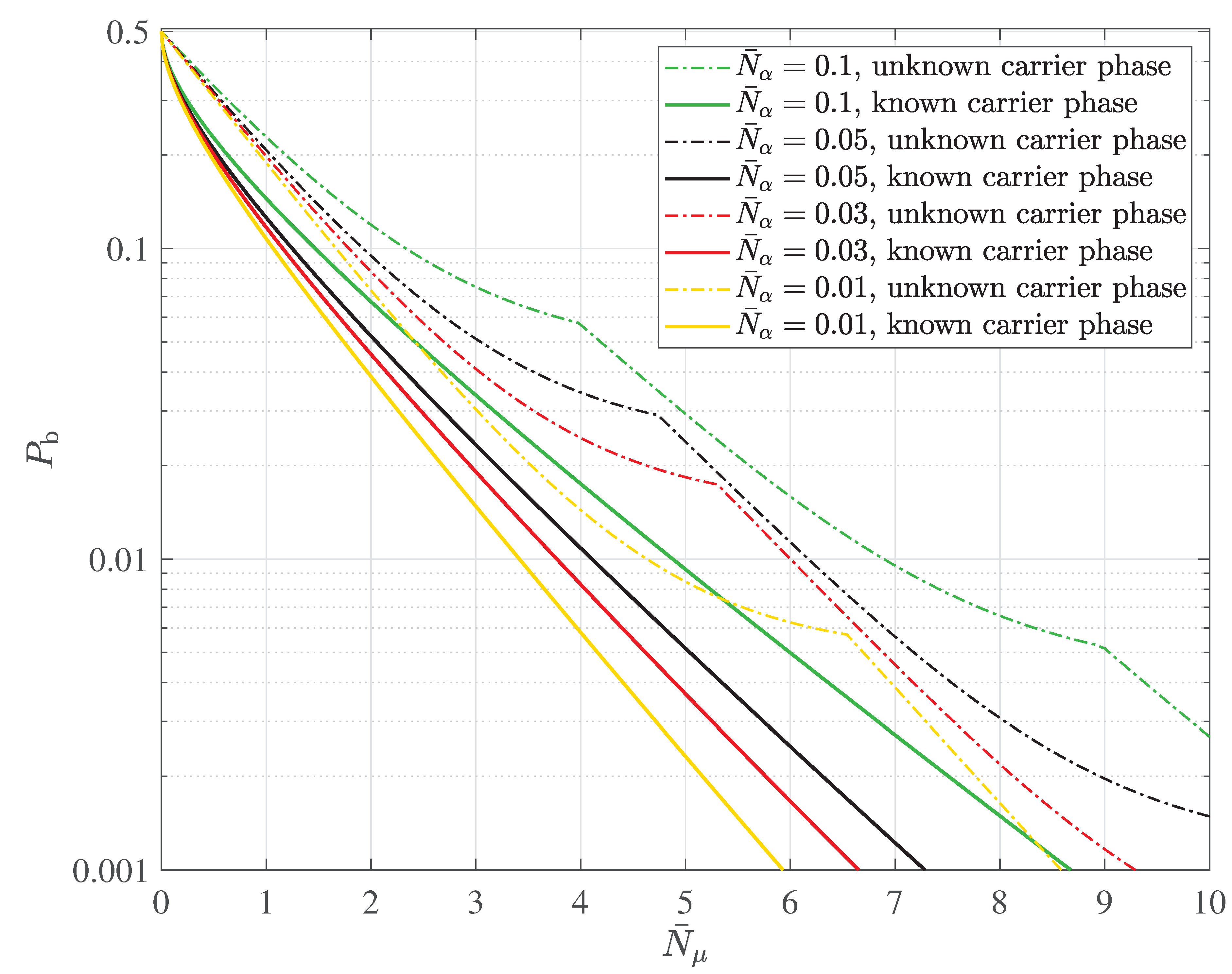
Next, we consider multipath transmission and reception under the presence of decoherence, see Section 2.4. The standardization of mobile radio systems has necessitated the development of widely accepted channel models, cf. e.g., [35,56,57]. Unfortunately, quantum communication systems, such as those discussed here, have not yet reached a comparable level of standardization. Consequently, commonly accepted multipath quantum channel models are not yet available. To proceed, we adopt multipath quantum channels with time-invariant channel impulse responses (CIRs), as first introduced in [55, Tab. 3.7, p. 662]. Specifically, we consider two distinct multipath quantum channels, referred to as CIR#4 and CIR#5 [55, Tab. 3.7, p. 662]. The corresponding CIR coefficients , , are listed in Table 1 [55, Tab. 3.7, p. 662]. The selected multipath quantum channels are assumed to be energy-preserving, that is, they neither amplify nor attenuate the transmitted signals. The CIRs of both CIR#4 and CIR#5 are normalized accordingly by ensuring
This guarantees that all depicted results are comparable in terms of average received energy. Consequently, if the laser remains continuously on, the average number of received signal photons is , regardless of the chosen channel model, see, e.g., (21).
Figure 12 shows a detail of simulation results of the uncoded BER performance versus the average number of signal photons per message bit with the average number of thermal photons as the curve parameter in the case of the transmission via the multipath quantum channel CIR#4, which has the two channel coefficients equal to and equal to . Similar to e.g. [6][Fig. 3, p. 1590], the average number of thermal noise photons was chosen from . Furthermore, Figure 13 illustrates a detail of simulation results of the uncoded BER performance versus the average number of signal photons per message bit with the average number of thermal photons as the curve parameter in the case of the transmission via the multipath quantum channel CIR#5, which has the three channel coefficients equal to , equal to and equal to . In both cases, the optimum quantum data detection schemes log-ML and SOVA are used. The uncoded BER curves obtained in the case of the log-ML are shown as solid lines while the uncoded BER curves determined in the case of the SOVA are depicted as dashed lines. As expected, the uncoded BER decreases monotonically with increasing for a given value of . Furthermore, the uncoded BER increases with increasing thermal noise, i.e. with increasing , for a given value of . Also, the steepness of the uncoded BER curves seems to decrease with increasing thermal noise, i.e. with increasing . Remarkably, for given values of and , the log-ML and the SOVA perform almost identically. In addition, compared with the multipath quantum channel CIR#4, the multipath quantum channel CIR#5 has a greater multipath spread. For given values of and , this leads to an increased uncoded BER in the case of the multipath quantum channel CIR#5 versus the multipath quantum channel CIR#4.
Figure 12.
Detail of simulation results of the uncoded bit error ratio (BER) performance versus the average number of signal photons per message bit with the average number of thermal photons as the curve parameter for the transmission via the multipath quantum channel CIR#4 with ; the optimum quantum data detection schemes log-ML (solid lines) and SOVA (dashed lines) are considered.
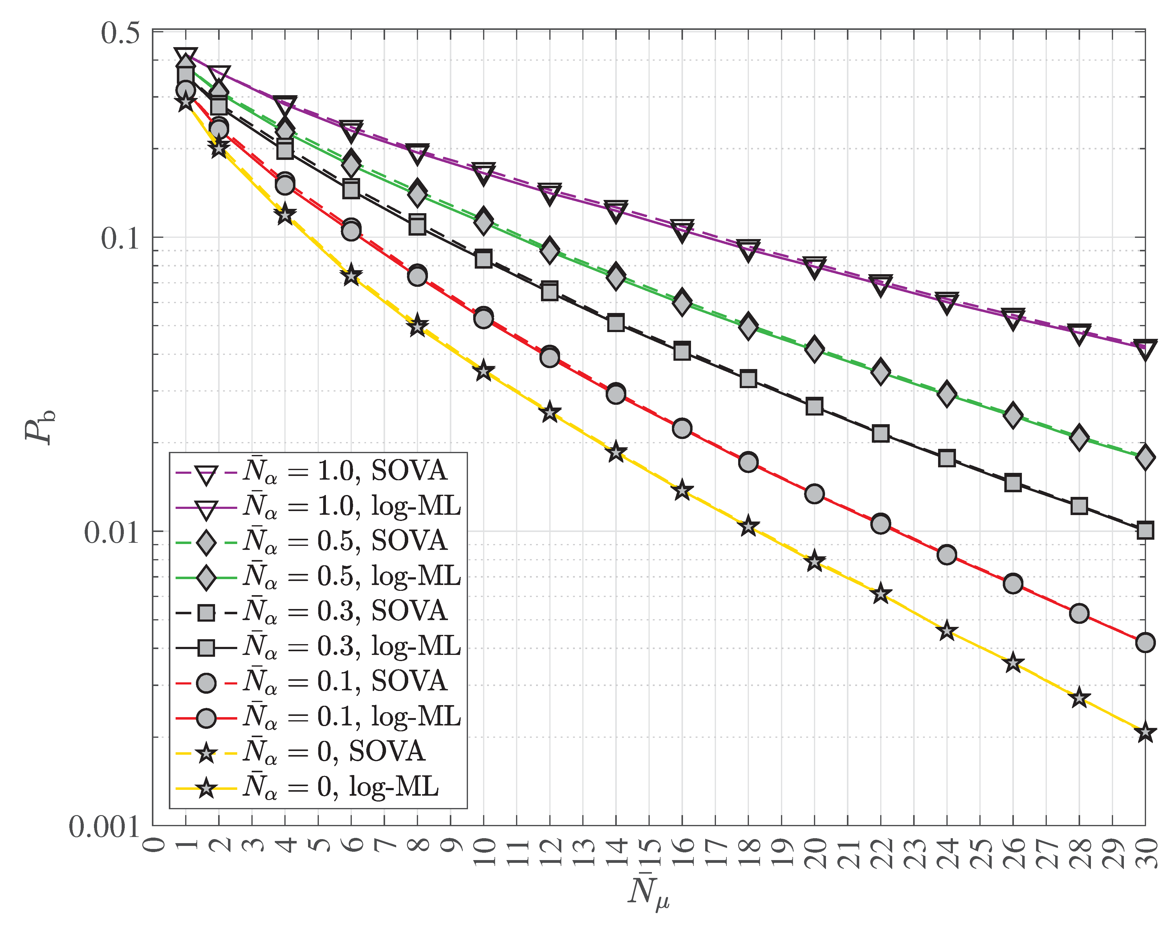
Figure 13.
Detail of simulation results of the uncoded bit error ratio (BER) performance versus the average number of signal photons per message bit with the average number of thermal photons as the curve parameter for the transmission via the multipath quantum channel CIR#5 with ; the optimum quantum data detection schemes log-ML (solid lines) and SOVA (dashed lines) are considered.
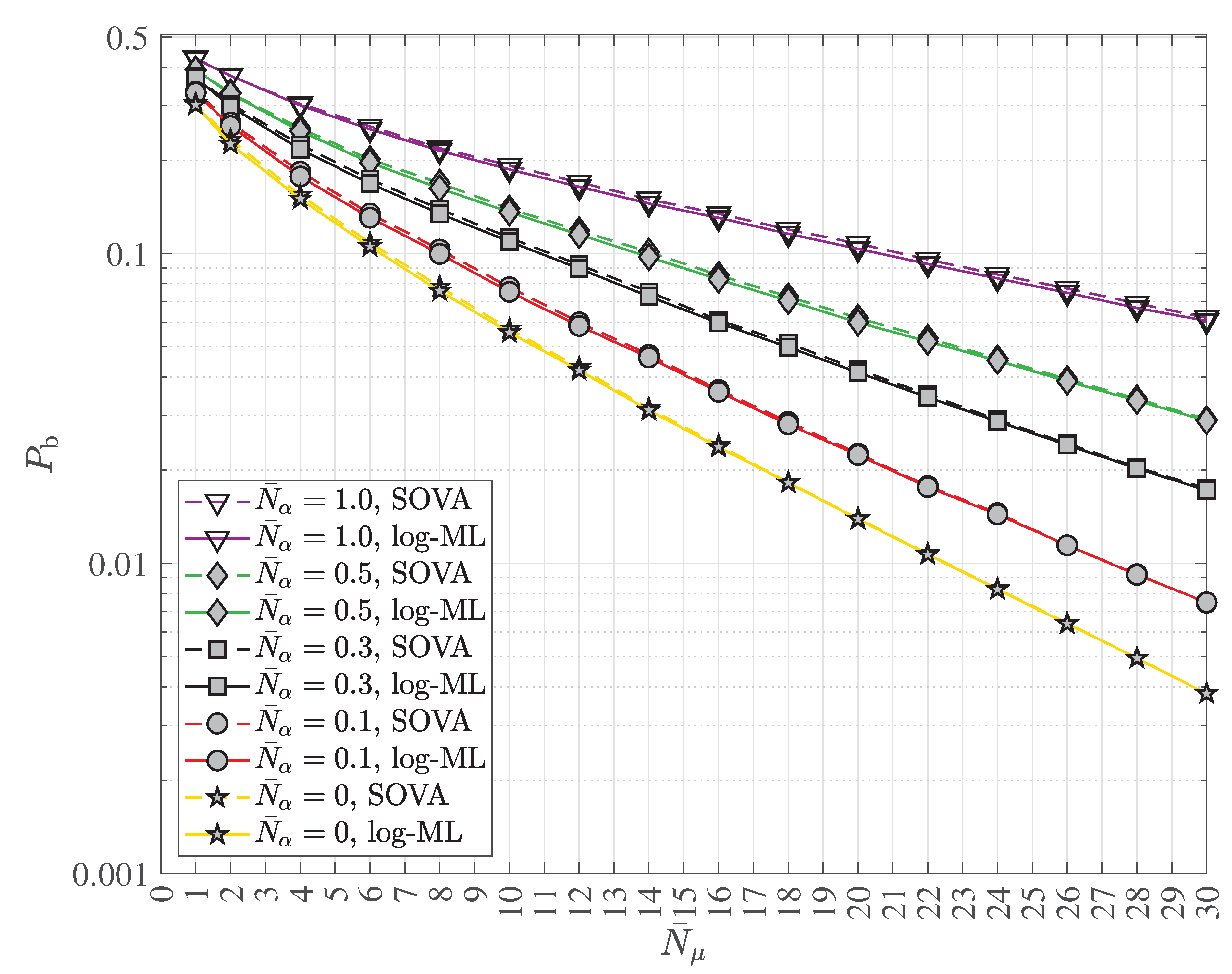
Figure 14 shows a detail of simulation results of the uncoded BER performance versus the average number of signal photons per message bit with the average number of thermal photons as the curve parameter in the case of the transmission via the multipath quantum channel CIR#5, having equal to 3 nonzero channel coefficients equal to , equal to and equal to , hence, three distinct paths. The reduced state quantum data detection schemes rslog-ML with equal to 2 and rsSOVA with equal to 2 are applied. The uncoded BER curves obtained in the case of the rslog-ML are shown as solid lines while the uncoded BER curves determined in the case of the rsSOVA are depicted as dashed lines. As expected, the uncoded BER decreases monotonically with increasing for a given value of . Furthermore, the uncoded BER increases with increasing thermal noise, i.e. with increasing , for a given value of . Also, the steepness of the uncoded BER curves seems to decrease with increasing thermal noise, i.e. with increasing . Remarkably, for given values of and , the rslog-ML and the rsSOVA perform almost identically. When comparing the Figure 13 and Figure 14, we realize that the performance degradation of the reduced state versions of the log-ML and the SOVA is small compared to the more complex log-ML and SOVA quantum data detectors.
Figure 14.
Detail of simulation results of the uncoded bit error ratio (BER) performance versus the average number of signal photons per message bit with the average number of thermal photons as the curve parameter for the transmission via the multipath quantum channel CIR#5 with ; the reduced state quantum data detection schemes rslog-ML with (solid lines) and rsSOVA with (dashed lines) are considered.
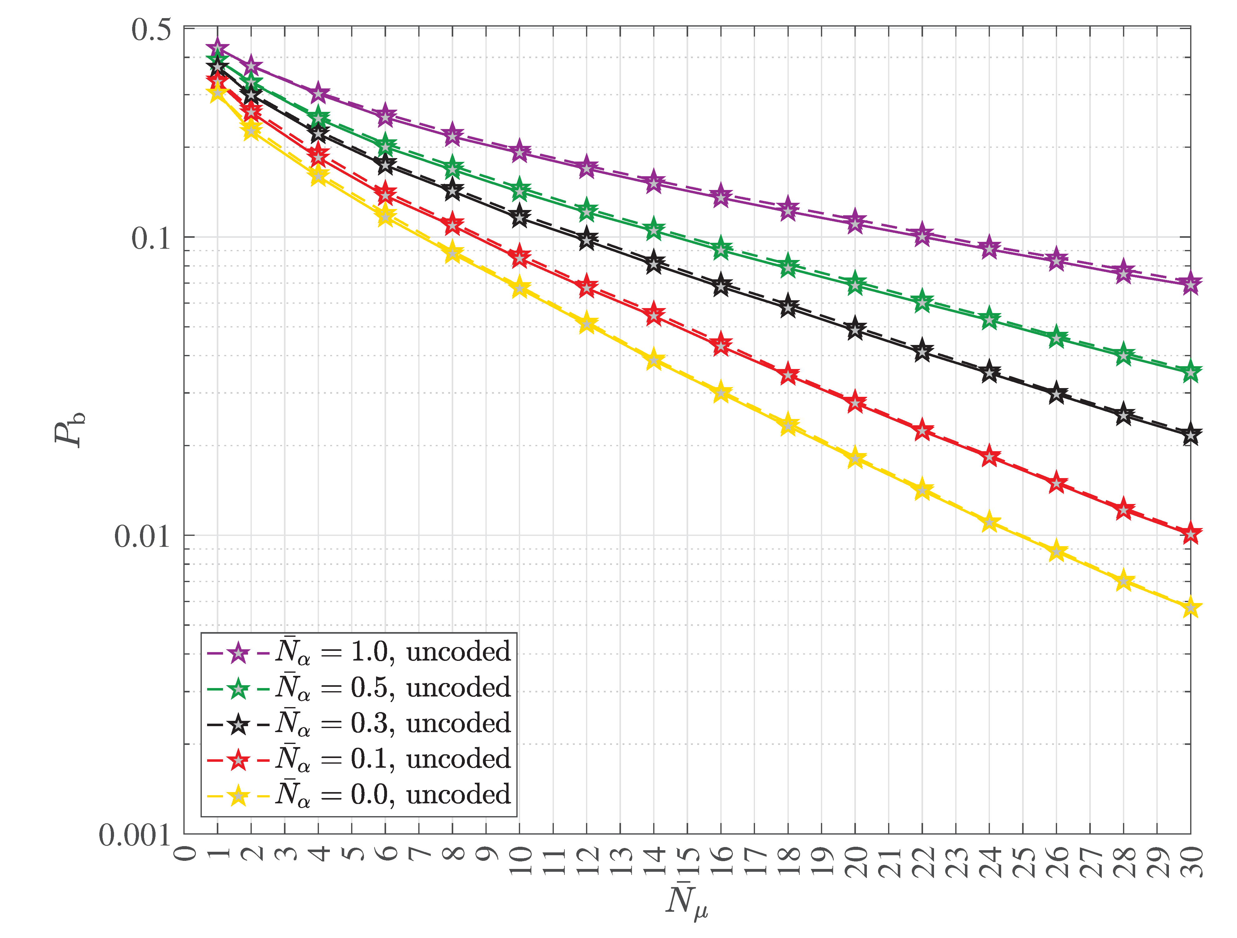
Figure 15 illustrates a detail of simulation results of the uncoded BER performance versus the average number of signal photons per message bit with the average number of thermal photons as the curve parameter for the transmission via the multipath quantum channel CIR#5 having equal to 3 nonzero channel coefficients equal to , equal to and equal to , hence, three distinct paths. The reduced state quantum data detection scheme decision feedback equalizer (DFE), obtained for equal to 1 from the rslog-ML, the rslog-MAP, the rsAPRI-SOVA or the rsSOVA, is used. As expected, the uncoded BER decreases monotonically with increasing for a given value of . Furthermore, the uncoded BER increases with increasing thermal noise, i.e. with increasing , for a given value of . Also, the steepness of the uncoded BER curves seems to decrease with increasing thermal noise, i.e. with increasing . The DFE has the least implementation complexity, however, suffers from some performance degradation in comparison with the more elaborate log-ML, SOVA, rslog-ML with equal to 2 and rsSOVA with equal to 2, cf. Figure 13 and Figure 14.
Figure 15.
Detail of the simulation results of the uncoded bit error ratio (BER) performance versus the average number of signal photons per message bit with the average number of thermal photons as the curve parameter for the transmission via the multipath quantum channel CIR#5 with ; the reduced state quantum data detection scheme decision feedback equalizer (DFE) with is considered.
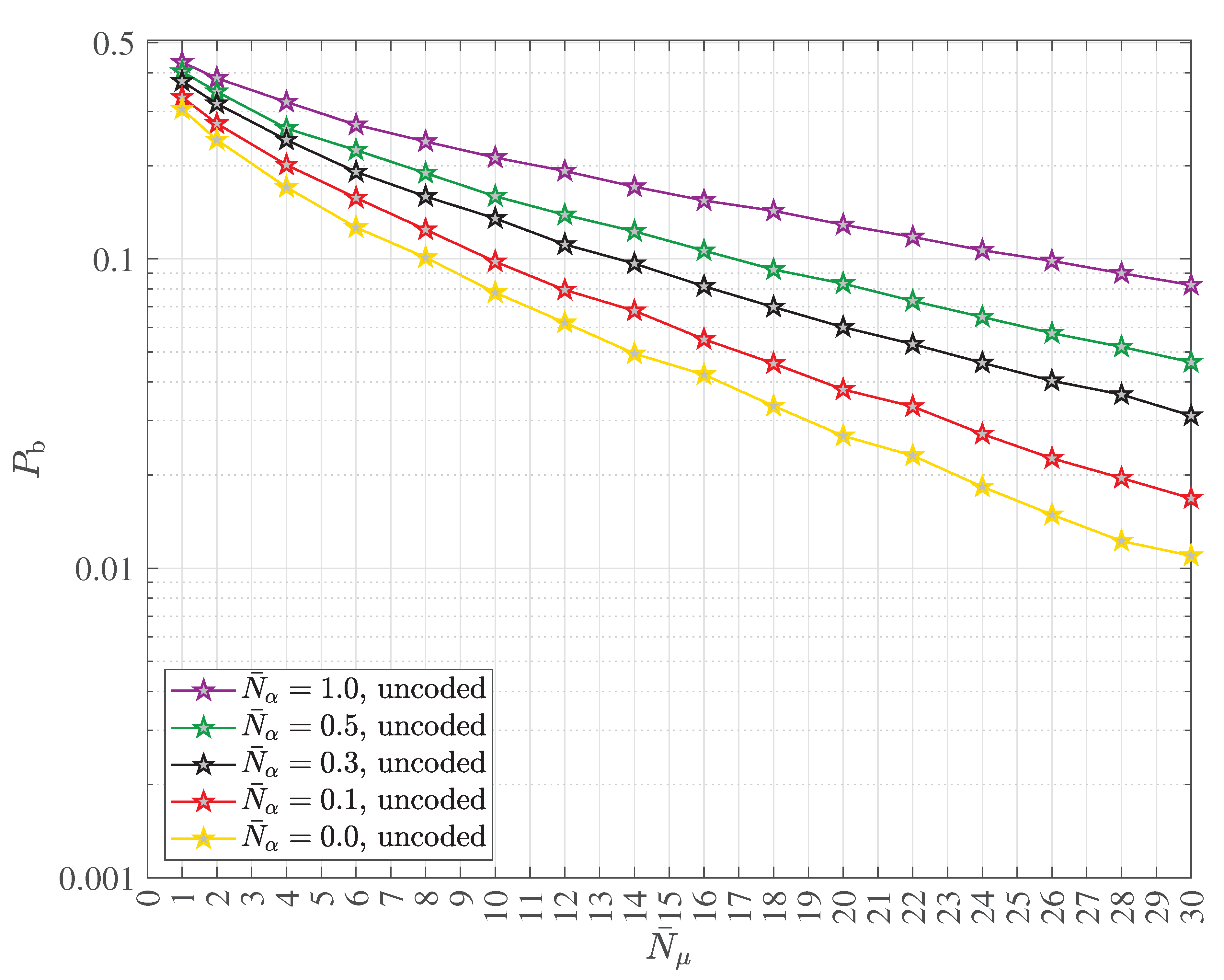
Figure 16 shows a detail of simulation results of the uncoded BER performance versus the average number of signal photons per message bit with the average number of thermal photons as the curve parameter for the transmission via the multipath quantum channel CIR#5 with is equal to 3. The performance of the log-ML quantum data detector (solid lines), the SOVA quantum data detector (dashed lines) and the Kohonen map based quantum data detector (solid lines with marker x) are shown for comparison. Obviously, for a given average number of thermal photons, the uncoded BER performance of the three considered quantum data detectors are almost identical.
Figure 16.
Detail of the simulation results of the uncoded bit error ratio (BER) performance versus the average number of signal photons per message bit with the average number of thermal photons as the curve parameter for the transmission via the multipath quantum channel CIR#5 with , comparing the performance of the log-ML quantum data detector (solid lines), the SOVA quantum data detector (dashed lines) and the Kohonen map based quantum data detector (solid lines with marker x).
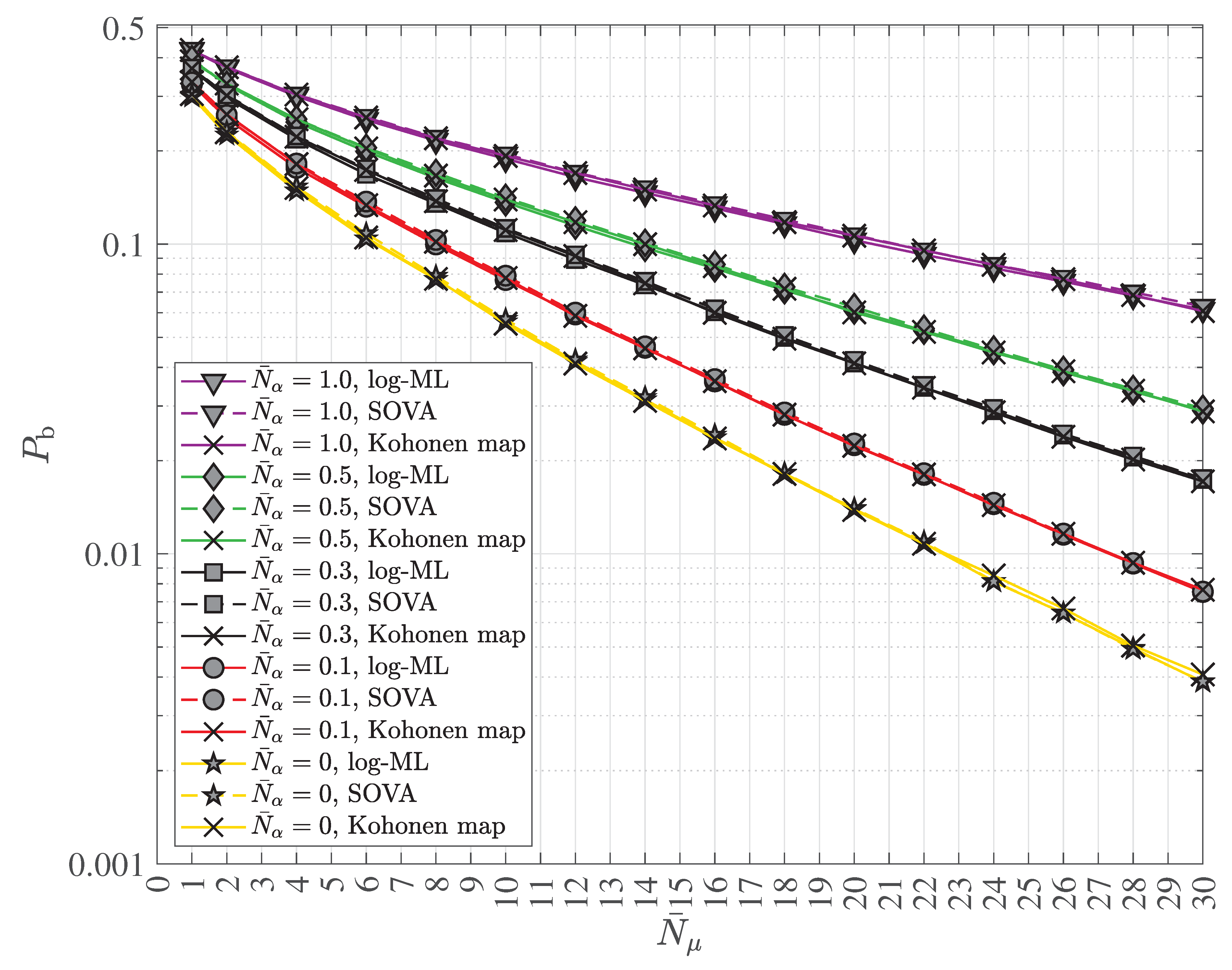
4.2. Coded Transmission and Reception Using the 3GPP Polar Code and Arikan’s Polar Code
Like in Section 4.1 we begin with the consideration of the short range transmission via a single path quantum channel CIR#1, cf. Table 1. Both the scenario without decoherence and, thus, with known carrier phase as well as the scenario subject to decoherence and, hence, with unknown carrier phase, the phase being a uniformly distributed random variable, have been evaluated by simulations in terms of
- the coded BER , i.e. the BER obtained after the channel decoding, and
- the BLER determined after the channel decoding.
The BLER is used as the performance measure because it has become one of the most important figures of merit in mobile communications systems and, in addition, the considered 5G/NR polar code protects control channels, which require the least possible BLER. The obtained detail of the coded BER performance is depicted in Figure 17 versus the average number of signal photons per message bit with the average number of thermal photons as the curve parameter. The obtained detail of the coded BLER performance versus the average number of signal photons per message bit with the average number of thermal photons as the curve parameter, corresponding to Figure 17, is shown in Figure 18. The dashed curves refer to the case of unknown carrier phase while the solid curves refer to the case of known carrier phase. We applied the 3GPP 5G/NR polar code with the generator matrix of (71) and the polar sequence of [41][Table 5.3.1.2-1, pp. 17-19], relying on 24 CRC bits generated with polynomial “24C”, code dimension K equal to 128, code length N equal to 256 and code rate equal to , i.e. . The average number of signal photons per message bit includes the code rate explicitly: is hence times greater than the average number of signal photons per codebit. The polar code decoding is accomplished with a CRC aided successive cancellation list (CA-SCL) decoder with list length L equal to 8. Interleaving between the channel encoder and the quantum mechanical harmonic oscillator is not deployed. The observations made are similar to those stated in the context of Figure 11, cf. Section 4.1. In any of the two scenarios, the coded BER , respectively the BLER , decreases monotonically with increasing for a given value of . Furthermore, the coded BER , respectively the BLER , increases with increasing thermal noise, i.e. with increasing , for a given value of . Remarkably, the coded BER , respectively the BLER , is always lower in the case of known carrier phase than in the case of unknown carrier phase for given values of and . Table 2 summarizes the estimated average number of signal photons per message bit required to obtain equal to and equal to associated with the results shown in Figure 17 and Figure 18.
Table 2.
Estimated average number of signal photons per message bit required to obtain and associated with the results shown in Figure 16 and Figure 17.
| BER, unknown | ||||
| BER, known carrier phase | ||||
| BLER, unknown | ||||
| BLER, known carrier phase |
Figure 17.
Detail of simulation results of the coded bit error ratio (BER) performance versus the average number of signal photons per message bit with the average number of thermal photons as the curve parameter; the dashed curves refer to the case of unknown carrier phase while the solid curves refer to the case of known carrier phase; the 3GPP 5G/NR polar code with the generator matrix of (71) and the polar sequence of [41][Table 5.3.1.2-1, pp. 17-19] is used with 24 CRC bits, code dimension , code length and code rate ; the code rate is explicitly included in ; the polar code decoding is accomplished with the CA-SCL decoder with list length ; interleaving is not deployed.
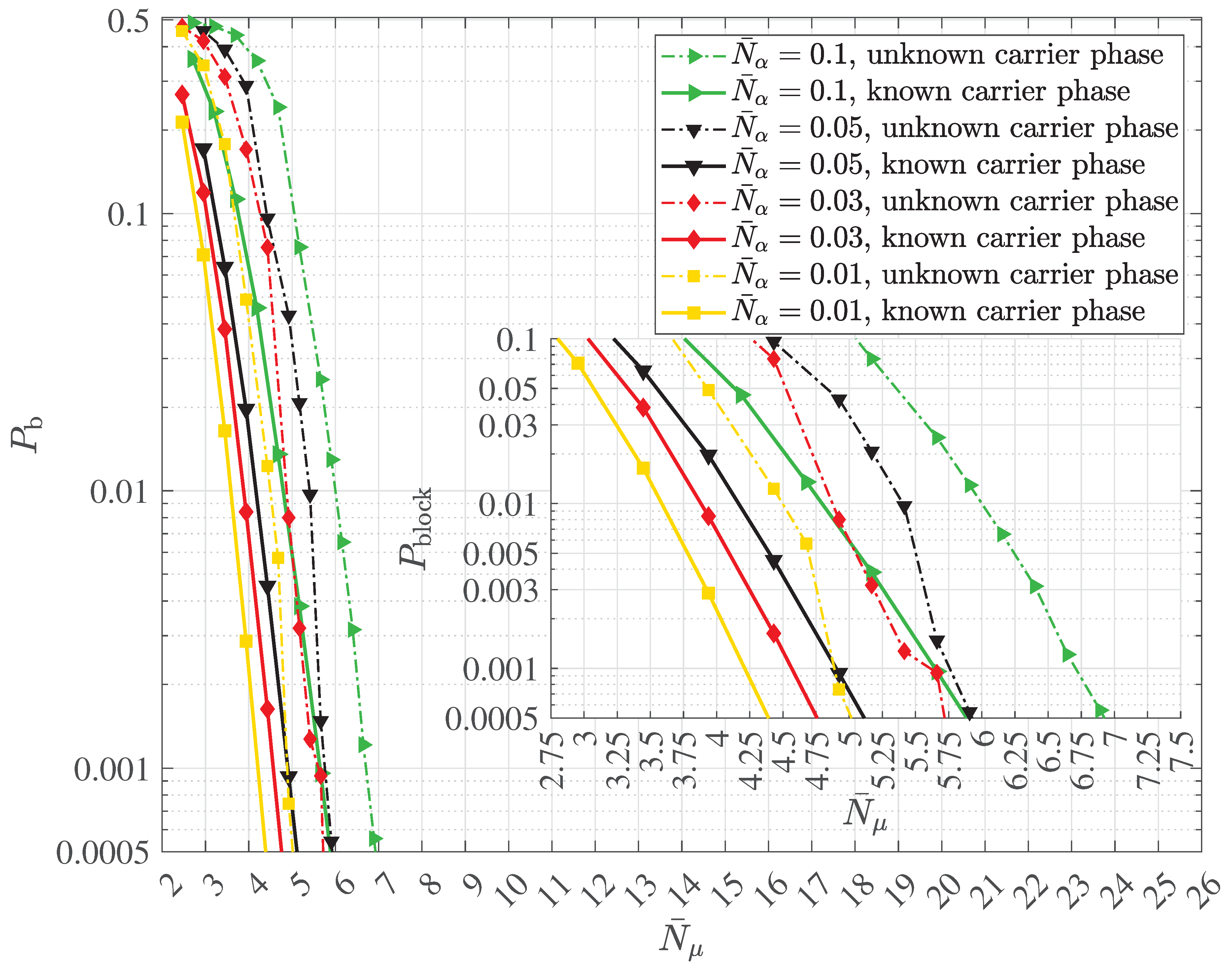
Figure 18.
Detail of simulation results of the block error ratio (BLER) performance versus the average number of signal photons per message bit with the average number of thermal photons as the curve parameter; the dashed curves refer to the case of unknown carrier phase while the solid curves refer to the case of known carrier phase; the 3GPP 5G/NR polar code with the generator matrix of (71) and the polar sequence of [41][Table 5.3.1.2-1, pp. 17-19] is used with 24 CRC bits generated using the polynomial “24C”, code dimension , code length and code rate ; the code rate is explicitly included in ; the polar code decoding is accomplished with the CA-SCL decoder having the list length ; interleaving is not deployed.
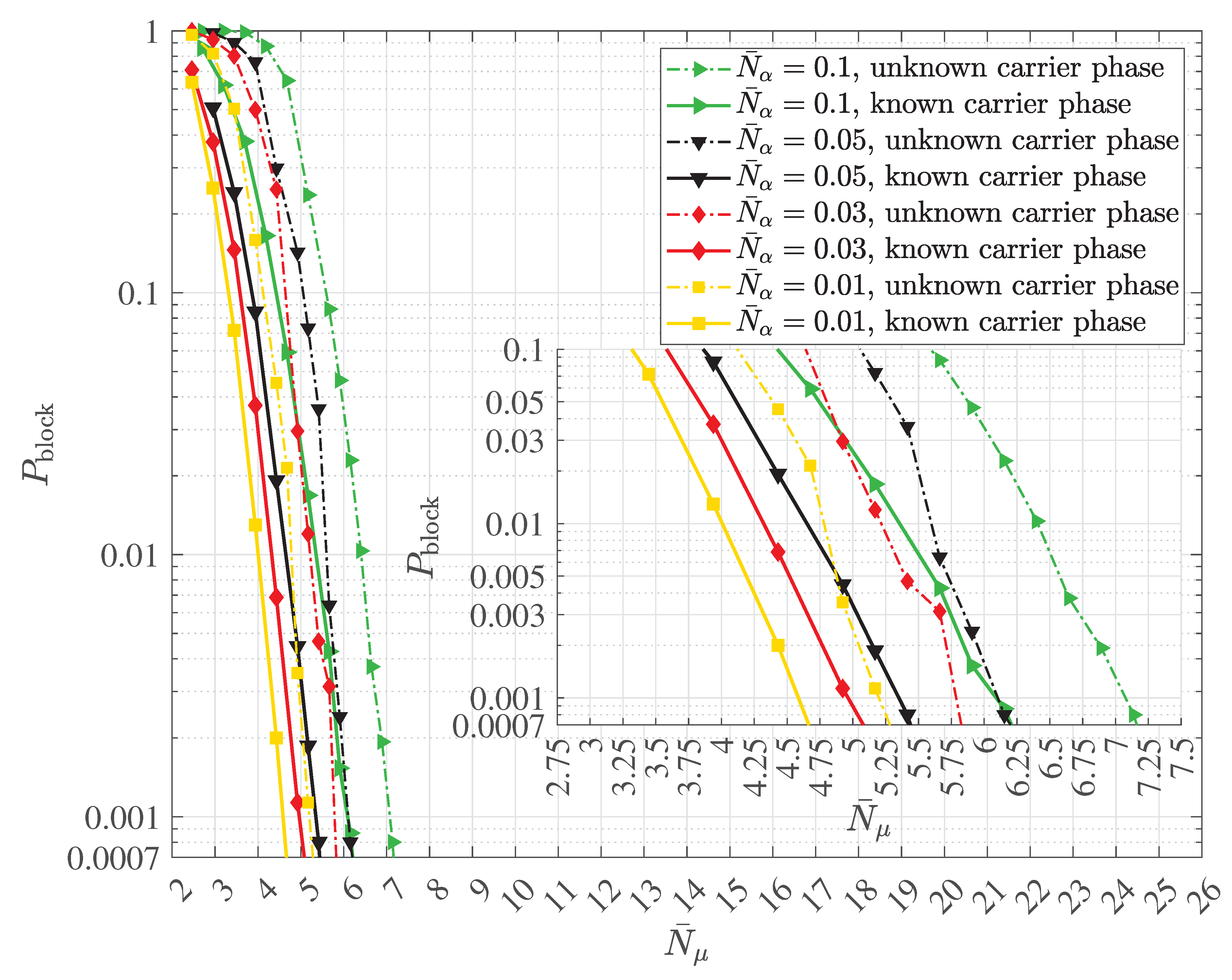
Figure 19 shows a detail of simulation results of the coded BER performance and Figure 20 shows a detail of simulation results of the BLER performance versus the average number of signal photons per message bit with the average number of thermal photons as the curve parameter for the transmission via the multipath quantum channel CIR#4 when the 3GPP 5G/NR polar code with the generator matrix of (71) and the polar sequence of [41][Table 5.3.1.2-1, pp. 17-19] is used. Figure 21 shows a detail of simulation results of the coded BER performance and Figure 22 shows a detail of simulation results of the BLER performance versus the average number of signal photons per message bit with the average number of thermal photons as the curve parameter for the transmission via the multipath quantum channel CIR#4 when the Arikan-style polar code with the generator matrix of (72) and the associated polar sequence generated by Arikan’s Bhattacharyya parameter based approach setting out from the binary erasure channel with erasure probability equal to , is used.
Figure 19.
Detail of simulation results of the coded bit error ratio (BER) performance versus the average number of signal photons per message bit with the average number of thermal photons as the curve parameter for the transmission via the multipath quantum channel CIR#4; log-ML quantum data detection is applied; the 3GPP 5G/NR polar code with the generator matrix of (74) and the polar sequence of [41][Table 5.3.1.2-1, pp. 17-19] is used; 24 CRC bits generated with polynomial “24C” are used; the polar code decoding is accomplished with the SC decoder, hence, CRC bits are not processed by the SC decoder; the code length N is 512; three choices of the code dimension, (—■—), (- - -▴- - -) and (- · -★- · -), leading to the three code rates = (171 - 24)/512 (—■—), = (256 - 24)/512 (- - -▴- - -) and = (410 - 24)/512 (- · -★- · -) are considered; the code rate is explicitly included in ; interleaving is deployed.
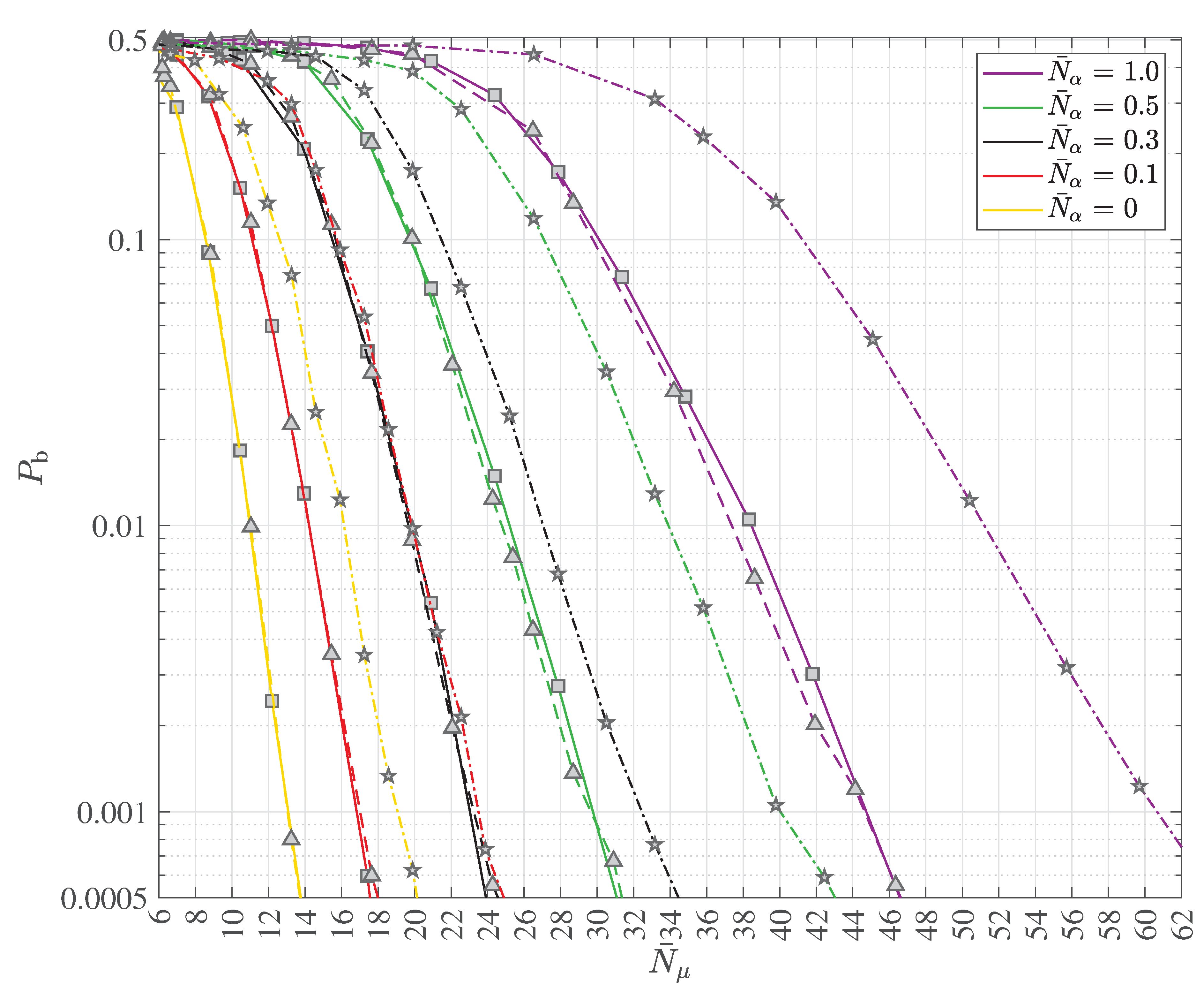
Figure 20.
Detail of simulation results of the block error ratio (BLER) performance versus the average number of signal photons per message bit with the average number of thermal photons as the curve parameter for the transmission via the multipath quantum channel CIR#4; log-ML quantum data detection is applied; the 3GPP 5G/NR polar code with the generator matrix of (71) and the polar sequence of [41][Table 5.3.1.2-1, pp. 17-19] is used; 24 CRC bits generated with polynomial “24C” are used; the polar code decoding is accomplished with the SC decoder, hence, CRC bits are not processed by the SC decoder; the code length N is 512; three choices of the code dimension, (—■—), (- - -▴- - -) and (- · -★- · -), leading to the three code rates = (171 - 24)/512 (—■—), = (256 - 24)/512 (- - -▴- - -) and = (410 - 24)/512 (- · -★- · -) are considered; the code rate is explicitly included in ; interleaving is deployed.
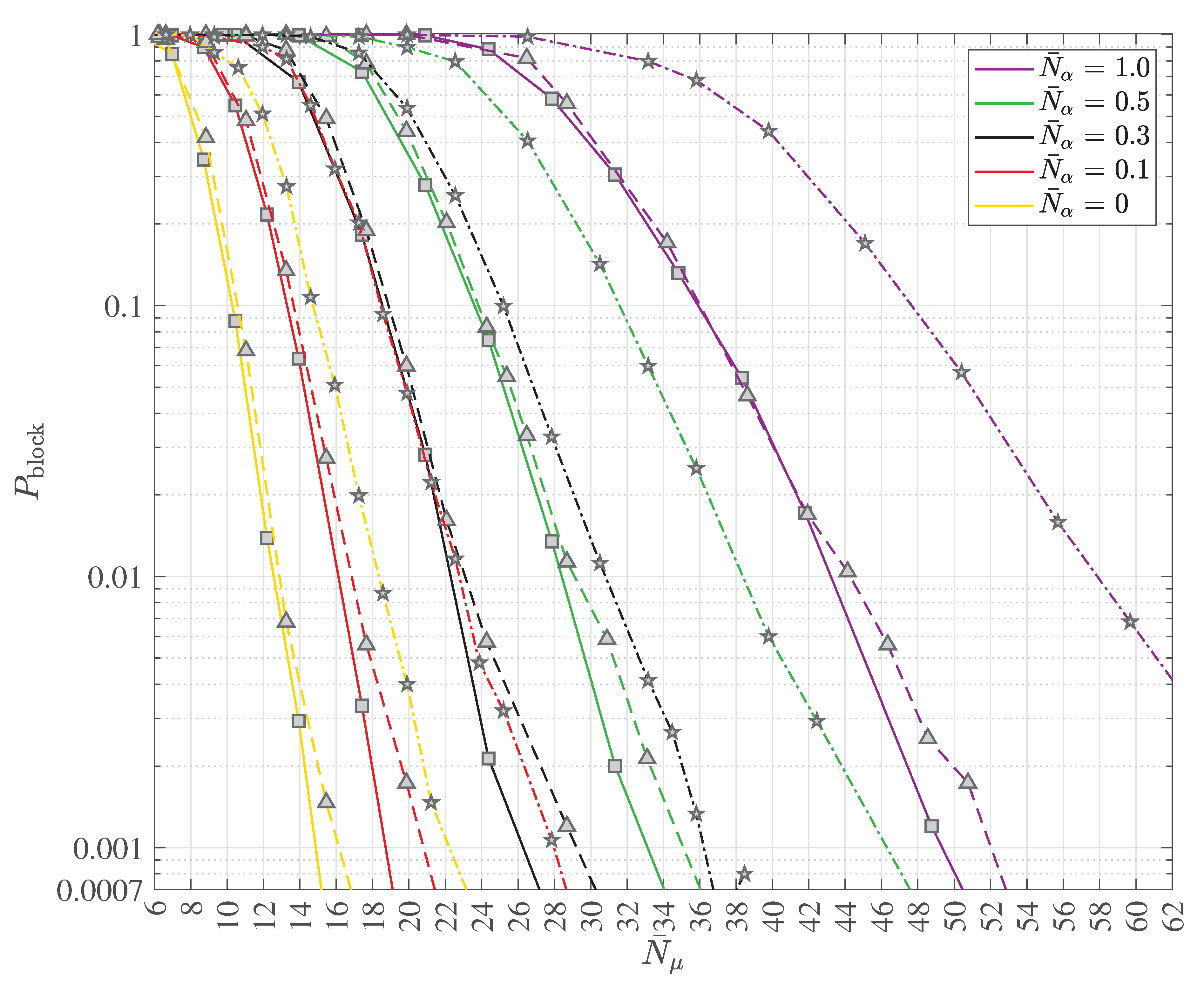
Figure 21.
Detail of simulation results of the coded bit error ratio (BER) performance versus the average number of signal photons per message bit with the average number of thermal photons as the curve parameter for the transmission via the multipath quantum channel CIR#4; log-ML quantum data detection is applied; the Arikan-style polar code with the generator matrix of (72) and the associated polar sequence generated by Arikan’s Bhattacharyya parameter based approach setting out from the binary erasure channel with erasure probability is used; 24 CRC bits generated with polynomial “24C” are used; the polar code decoding is accomplished with the SC decoder, hence, CRC bits are not processed by the SC decoder; the code length N is 512; three choices of the code dimension, (—■—), (- - -▴- - -) and (- · -★- · -), leading to the three code rates = (171 - 24)/512 (—■—), = (256 - 24)/512 (- - -▴- - -) and = (410 - 24)/512 (- · -★- · -) are considered; the code rate is explicitly included in ; interleaving is deployed.
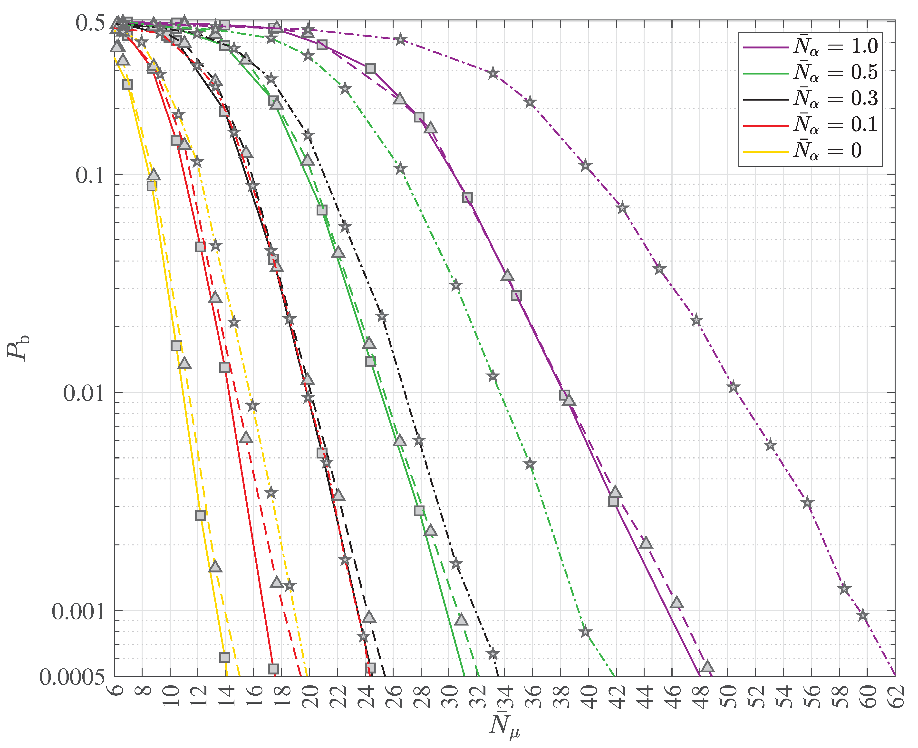
Figure 22.
Detail of simulation results of the block error ratio (BLER) performance versus the average number of signal photons per message bit with the average number of thermal photons as the curve parameter for the transmission via the multipath quantum channel CIR#4; log-ML quantum data detection is applied; the Arikan-style polar code with the generator matrix of (72) and the associated polar sequence generated by Arikan’s Bhattacharyya parameter based approach setting out from the binary erasure channel with erasure probability is used; 24 CRC bits generated with polynomial “24C” are used; the polar code decoding is accomplished with the SC decoder, hence, CRC bits are not processed by the SC decoder; the code length N is 512; three choices of the code dimension, (—■—), (- - -▴- - -) and (- · -★- · -), leading to the three code rates = (171 - 24)/512 (—■—), = (256 - 24)/512 (- - -▴- - -) and = (410 - 24)/512 (- · -★- · -) are considered; the code rate is explicitly included in ; interleaving is deployed.
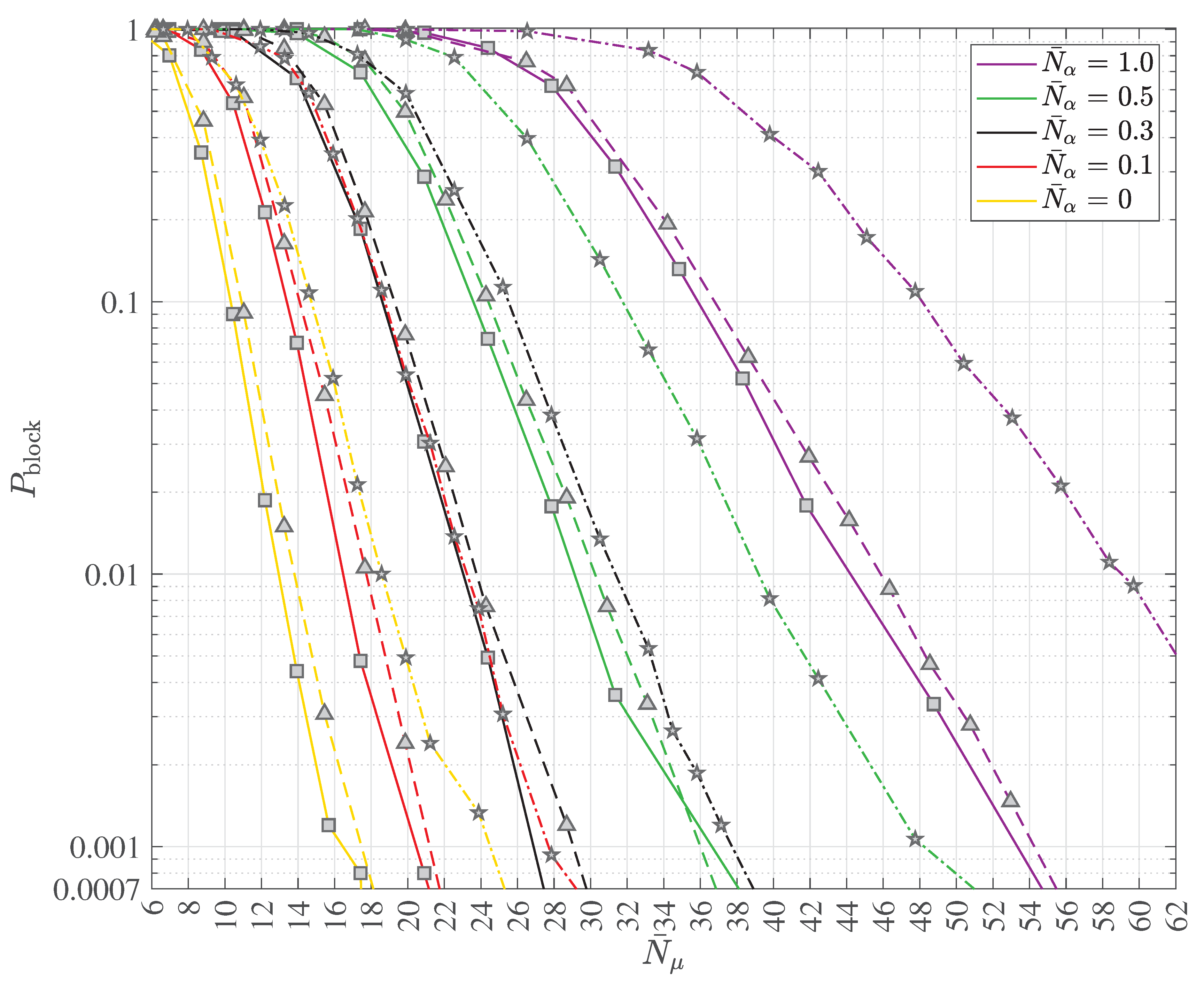
Similar to e.g. [6][Fig. 3, p. 1590], the average number of thermal noise photons was chosen from . In all cases, log-ML quantum data detection is applied. 24 CRC bits generated with polynomial “24C” are used. The polar code decoding is accomplished with the SC decoder, hence, CRC bits are not processed by the SC decoder. The code length N is equal to 512. Furthermore, three choices of the code dimension, K equal to 171 (—■—), K equal to 256 (- - -▴- - -) and K equal to 410 (- · -★- · -), leading to the three code rates equal to , i.e. (—■—), equal to , i.e. (- - -▴- - -) and equal to , i.e. (- · -★- · -) are considered. Of course, the code rate is explicitly included in . Interleaving according to the illustration in Section 3.3 was deployed. Both the coded BER , respectively the BLER , decreases monotonically with increasing for a given value of . Furthermore, the coded BER , respectively the BLER , increases with increasing thermal noise, i.e. with increasing , for a given value of . It can be seen that the considered polar code performs almost identical for code rates lower than or equal to . However, for higher code rates an increasing number of virtual channels with low channel capacity are used, which leads to considerable performance degredations. The said degradations increase with increasing . Table 3 summarizes the estimated average number of signal photons required to obtain equal to and equal to associated with the results shown in Figure 19, Figure 20, Figure 21 and Figure 22.
Table 3.
Estimated average number of signal photons per message bit required to obtain and associated with the results shown in Figure 18, Figure 19, Figure 20 and Figure 21.
| polar code | |||||||
|---|---|---|---|---|---|---|---|
| BER | 3GPP 5G/NR | ||||||
| BER | Arikan | ||||||
| BER | 3GPP 5G/NR | ||||||
| BER | Arikan | ||||||
| BER | 3GPP 5G/NR | ||||||
| BER | Arikan | ||||||
| BLER | 3GPP 5G/NR | ||||||
| BLER | Arikan | ||||||
| BLER | 3GPP 5G/NR | ||||||
| BLER | Arikan | ||||||
| BLER | 3GPP 5G/NR | ||||||
| BLER | Arikan |
Like in Section 4.1, let us concentrate on multipath transmission and reception under the presence of decoherence, see Section 2.4. Again, we consider the two distinct multipath quantum channels CIR#4 and CIR#5 of Table 1 [55, Tab. 3.7, p. 662]. Figure 23 and Figure 24 illustrate the details of simulation results of the BLER performance versus the average number of signal photons with the average number of thermal photons as the curve parameter for the transmission via the multipath quantum channels CIR#4 and CIR#5. Again, the 3GPP 5G/NR polar code with the generator matrix of (71) and the polar sequence of [41][Table 5.3.1.2-1, pp. 17-19] was used with 24 CRC bits generated with polynomial “24C”, having the code dimension K equal to 164, the code length N equal to 512 and, hence, the code rate equal to , i.e. . The code rate is explicitly included in , see above. Again, the polar code decoding is accomplished with the CA-SCL decoder having the list length L equal to 8. Interleaving between the channel encoder and the quantum mechanical harmonic oscillator is not deployed. The quantum data detectors log-ML (—■—), max*-log-ML (—▴—), max-log-ML (—★—), SOVA with the BATTAIL RULE (BR) (- - -•- - -), SOVA with the HUBER RULE (HR) (- - -▾- - -) and SOVA with the SIMPLE RULE (SR) (- - -*- - -) are considered.
Figure 23.
Detail of simulation results of the block error ratio (BLER) performance versus the average number of signal photons per message bit with the average number of thermal photons as the curve parameter for the transmission via the multipath quantum channel CIR#4; the 3GPP 5G/NR polar code with the generator matrix of (71) and the polar sequence of [41][Table 5.3.1.2-1, pp. 17-19] is used with 24 CRC bits generated with polynomial “24C”, code dimension , code length , code rate ; the code rate is explicitly included in ; the polar code decoding is accomplished with the CA-SCL decoder having the list length ; interleaving is not deployed; associating the curves with the quantum data detectors is as follows: —▪—: log-ML; —▴—: max*-log-ML; —★—: max-log-ML; - - -•- - -: SOVA w/ BATTAIL RULE (BR); - - -▾- - -: SOVA w/ HUBER RULE (HR); - - -*- - -: SOVA w/ SIMPLE RULE (SR).
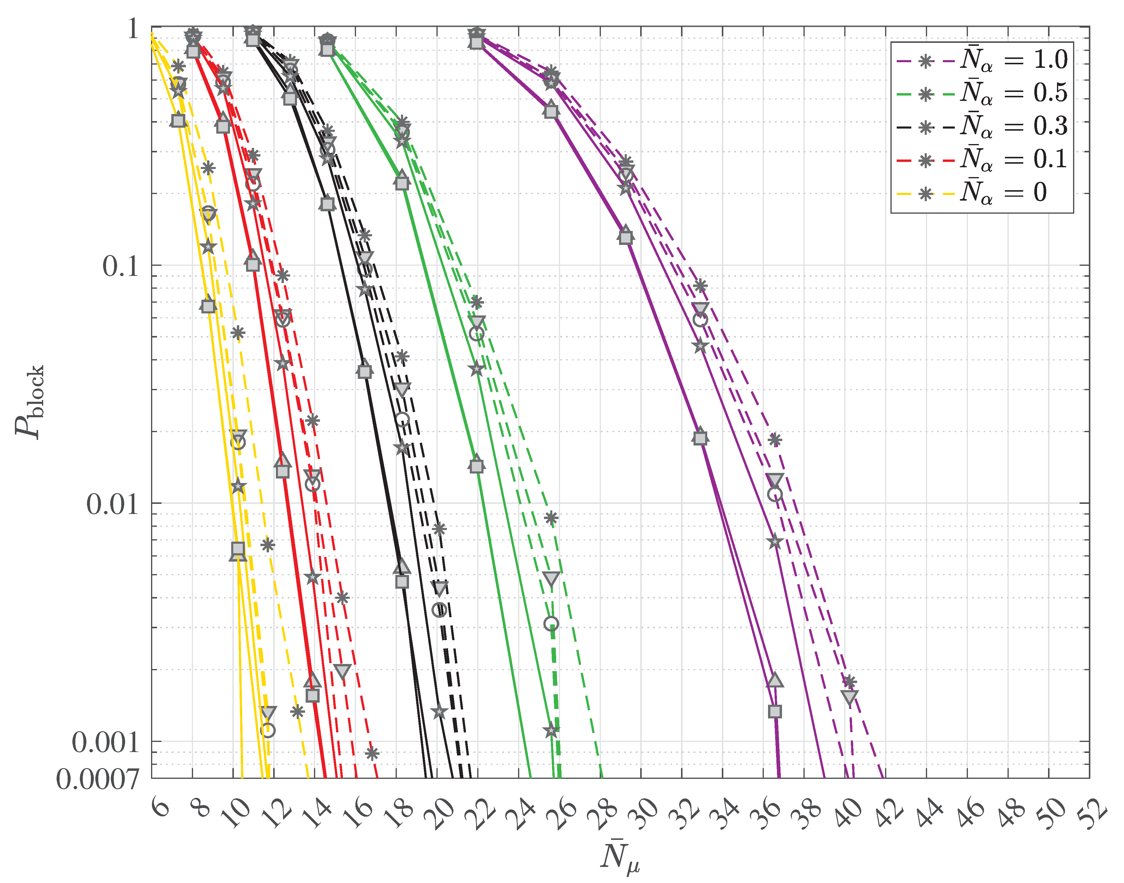
Figure 24.
Detail of simulation results of the block error ratio (BLER) performance versus the average number of signal photons per message bit with the average number of thermal photons as the curve parameter for the transmission via the multipath quantum channel CIR#5; the 3GPP 5G/NR polar code with the generator matrix of (71) and the polar sequence of [41][Table 5.3.1.2-1, pp. 17-19] is used with 24 CRC bits generated with polynomial “24C”, code dimension , code length , code rate ; the code rate is explicitly included in ; the polar code decoding is accomplished with the CA-SCL decoder having the list length ; interleaving is not deployed; associating the curves with the quantum data detectors is as follows: —■—: log-ML; —▴—: max*-log-ML; —★—: max-log-ML; - - -•- - -: SOVA w/ BATTAIL RULE (BR); - - -▾- - -: SOVA w/ HUBER RULE (HR); - - -*- - -: SOVA w/ SIMPLE RULE (SR).
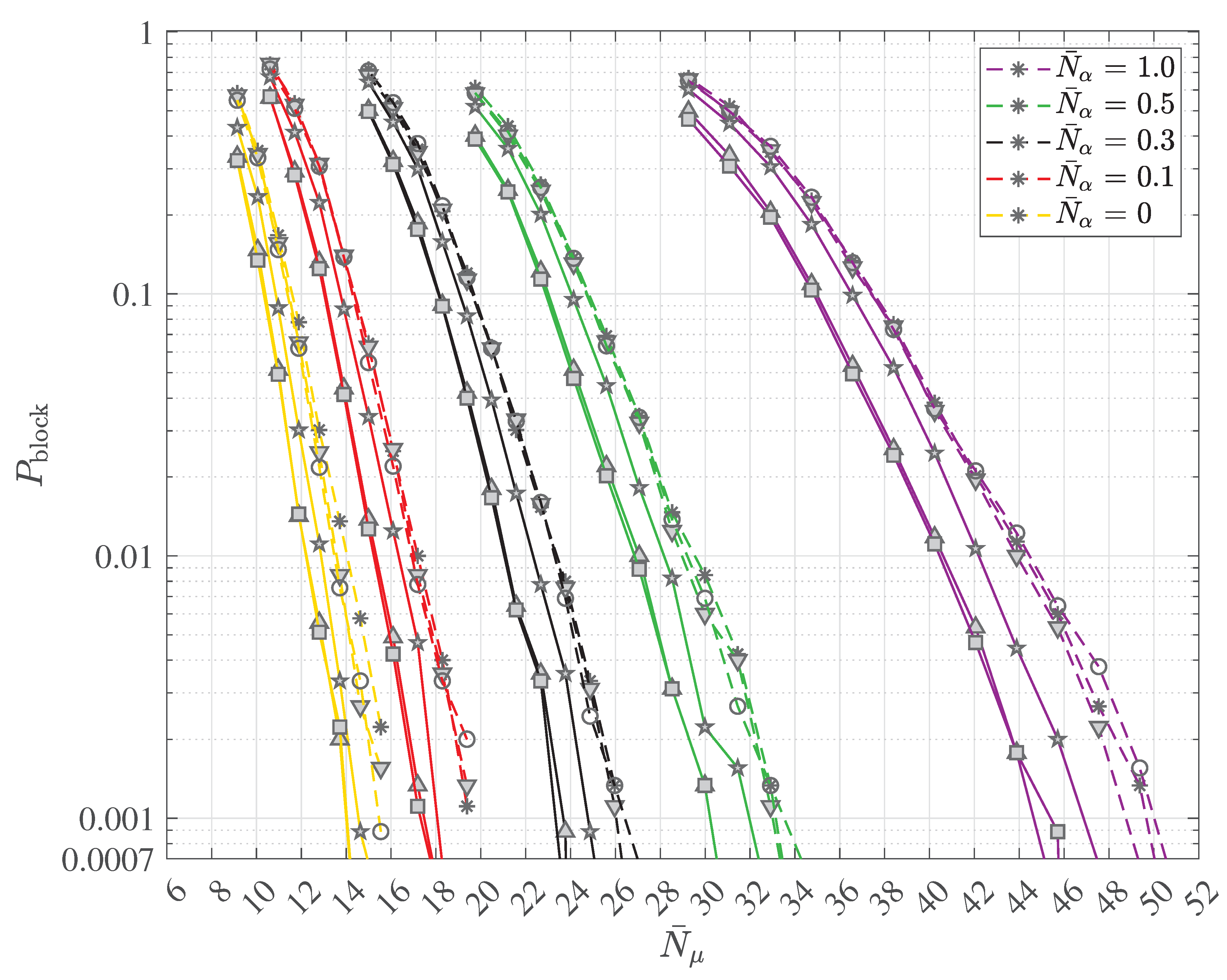
Similar to e.g. [6][Fig. 3, p. 1590], the average number of thermal noise photons was chosen from . The BLER performance obtainable with the six optimum quantum data detectors discussed in Section 2.4 for equal to is compared. It can be seen that for a given value of , the log-ML usually performs best and the max*-log-ML exploiting [17][Fig. 3.83, p. 473] provides nearly the same performance. Next comes the max-log-ML. As expected, the three SOVA variants are worse than the log-ML quantum data detectors. Table 4 summarizes the estimated average number of signal photons required to obtain equal to associated with the results shown in Figure 23 and Figure 24.
Table 4.
Estimated average number of signal photons per message bit required to obtain associated with the results shown in Figure 22 and Figure 23; the code rate is approximately equal to ; the symbol ≲ is used to indicate extrapolated values.
| channel | detector | |||||
|---|---|---|---|---|---|---|
| CIR#4 | SOVA, SR | |||||
| CIR#4 | SOVA, HR | |||||
| CIR#4 | SOVA, BR | |||||
| CIR#4 | max-log-ML | |||||
| CIR#4 | max*-log-ML | |||||
| CIR#4 | log-ML | |||||
| CIR#5 | SOVA, SR | |||||
| CIR#5 | SOVA, HR | |||||
| CIR#5 | SOVA, BR | |||||
| CIR#5 | max-log-ML | |||||
| CIR#5 | max*-log-ML | |||||
| CIR#5 | log-ML |
Figure 25 and Figure 26 illustrate selected simulation results showing the viability of the soft output Kohonen map based quantum data detection scheme (-·-x-·-) in comparison with the quantum data detectors log-ML (—■—), max*-log-ML (—▴—), max-log-ML (—★—), SOVA with the BATTAIL RULE (BR) (- - -•- - -), SOVA with the HUBER RULE (HR) (- - -▾- - -) and SOVA with the SIMPLE RULE (SR) (- - -*- - -). It is obvious that the soft output Kohonen map based quantum data detection scheme, which relies on the SR also applied in the SOVA with the SR, performs almost identical to this SOVA with the SR. Clearly, the soft output Kohonen map based quantum data detection scheme is an interesting alternative to the other quantum data detectors considered in this manuscript.
Figure 25.
Detail of simulation results of the block error ratio (BLER) performance versus the average number of signal photons per message bit with the average number of thermal photons equal to 0 for the transmission via the multipath quantum channel CIR#5; the 3GPP 5G/NR polar code with the generator matrix of (71) and the polar sequence of [41][Table 5.3.1.2-1, pp. 17-19] is used with 24 CRC bits generated with polynomial “24C”, code dimension , code length , code rate ; the code rate is explicitly included in ; the polar code decoding is accomplished with the CA-SCL decoder having the list length ; interleaving is not deployed; associating the curves with the quantum data detectors is as follows: -·-x-·-: Kohonen map; —■—: log-ML; —▴—: max*-log-ML; —★—: max-log-ML; - - -•- - -: SOVA w/ BATTAIL RULE (BR); - - -▾- - -: SOVA w/ HUBER RULE (HR); - - -*- - -: SOVA w/ SIMPLE RULE (SR).
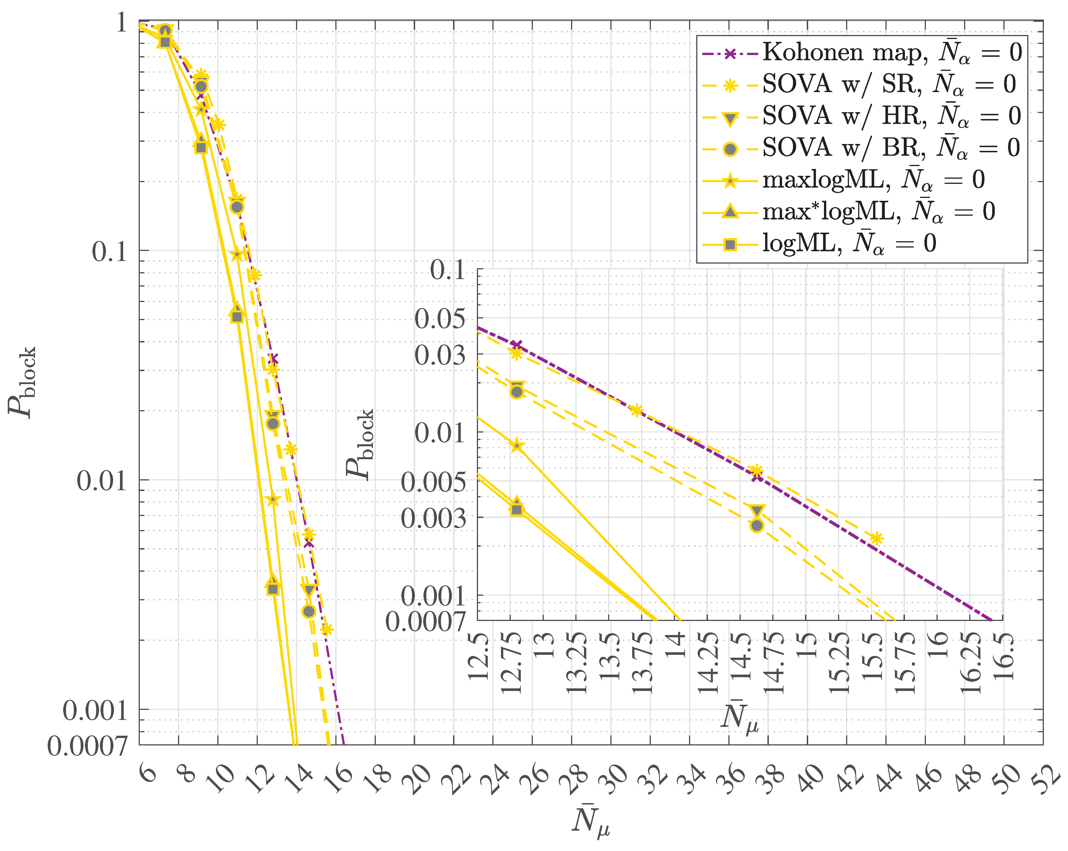
Figure 26.
Detail of simulation results of the coded bit error ratio (BER) performance versus the average number of signal photons per message bit with the average number of thermal photons equal to 0 for the transmission via the multipath quantum channel CIR#5; the 3GPP 5G/NR polar code with the generator matrix of (71) and the polar sequence of [41][Table 5.3.1.2-1, pp. 17-19] is used with 24 CRC bits generated with polynomial “24C”, code dimension , code length , code rate ; the code rate is explicitly included in ; the polar code decoding is accomplished with the CA-SCL decoder having the list length ; interleaving is not deployed; associating the curves with the quantum data detectors is as follows: -·-x-·-: Kohonen map; —■—: log-ML; —▴—: max*-log-ML; —★—: max-log-ML; - - -•- - -: SOVA w/ BATTAIL RULE (BR); - - -▾- - -: SOVA w/ HUBER RULE (HR); - - -*- - -: SOVA w/ SIMPLE RULE (SR).
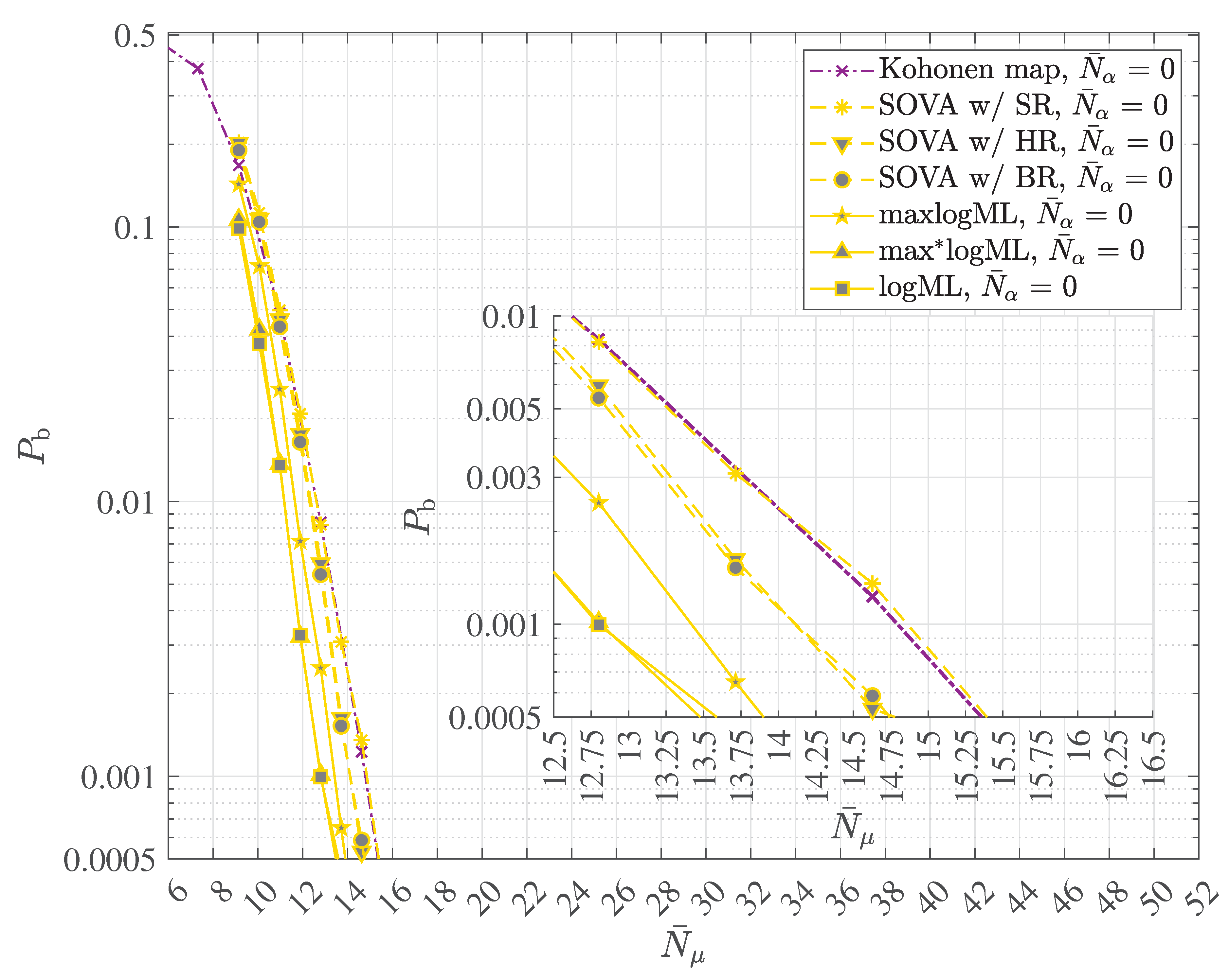
4.3. Optimzed Polar Sequence
Table 5 presents the estimated average number of signal photons per message bit received via the single path quantum channel CIR#1 required to obtain the BLER equal to . The 3GPP 5G/NR polar code with the generator matrix of (71) and either the 3GPP 5G/NR polar sequence of [41][Table 5.3.1.2-1, pp. 17-19], the polar sequence using p equal to , the newly generated polar sequence using p equal to (- - -▴- - -), cf. Algorithm 1, the newly generated polar sequence using p equal to (- · -★- · -), cf. Algorithm 1, or the newly generated polar sequence combining the polar sequences using p equal to and p equal to (), cf. Algorithm 2, is used. Since SC decoding is applied, no CRC bits are required. The code length was N equal to 256. The three code dimensions K equal to 86, K equal to 128 and K equal to 205, yielding the three code rates equal to , i.e. , equal to , i.e. , and equal to , i.e. are selected. Of course, the code rate is explicitly included in . We find that although the 3GPP polar sequence of [41][Table 5.3.1.2-1, pp. 17-19] facilitates an excellent BLER performance, already, improvements are still possible.
Table 5.
Estimated average number of signal photons per message bit received via the single path quantum channel CIR#1 required to obtain ; the 3GPP 5G/NR polar code with the generator matrix of (71) is used.
Table 5.
Estimated average number of signal photons per message bit received via the single path quantum channel CIR#1 required to obtain ; the 3GPP 5G/NR polar code with the generator matrix of (71) is used.
| carrier | |||||||
|---|---|---|---|---|---|---|---|
| phase | polar sequence | ||||||
| known | 3GPP 5G/NR | ||||||
| known | |||||||
| known | |||||||
| known | |||||||
| known | & | ||||||
| known | 3GPP 5G/NR | ||||||
| known | |||||||
| known | |||||||
| known | |||||||
| known | & | ||||||
| known | 3GPP 5G/NR | ||||||
| known | |||||||
| known | |||||||
| known | |||||||
| known | & | ||||||
| unknown | 3GPP 5G/NR | ||||||
| unknown | |||||||
| unknown | |||||||
| unknown | |||||||
| unknown | & | ||||||
| unknown | 3GPP 5G/NR | ||||||
| unknown | |||||||
| unknown | |||||||
| unknown | |||||||
| unknown | & | ||||||
| unknown | 3GPP 5G/NR | ||||||
| unknown | |||||||
| unknown | |||||||
| unknown | |||||||
| unknown | & |
4.4. Turbo Equalization with Polar Codes
In this Section 4.4, the performance that can be achieved by applying turbo equalization discussed in Section 3.3 will be illustrated.
Figure 27 shows the detail of simulation results of the coded BER performance and Figure 28 illustrates the detail of simulation results of the BLER performance versus the average number of signal photons per message bit with the average number of thermal photons equal to 0 for the transmission via the multipath quantum channel CIR#5 when turbo equalization with at most 20 iterations is taken into account, alternatively using the extrinsic soft output vector of (92), denoted by in the legend of Figure 27, respectively Figure 28, and according to (93), denoted by in the legend of Figure 27, respectively Figure 28. The expression “1st iteration“ in the legends of Figure 27 and Figure 28 refers to a single pass beginning at the quantum data detector via the optional deinterleaver and terminating at the polar code decoder, decoding the message , which is passed on to later receiver stages, cf. Figure 10. The polar code decoding is accomplished with the original SC decoder proposed by Arikan [39], hence, no CRC bits are required for the decoding. However, the CRC bits are used for the termination control of the turbo equalization. The original Arikan polar code is applied with the generator matrix of (71) and the polar sequence generated by applying Arikan’s Bhattacharyya parameter based approach, setting out from the binary erasure channel with erasure probability equal to . The code dimension K equals 88, the code length N is equal to 128, thus, the code rate equals , i.e. . In addition, block interleaving according to the illustration in Section 3.3 was deployed. As usual, the code rate is explicitly included in . As expected, the coded BER , respectively the BLER , decreases monotonically with increasing for a given value of . Remarkably, the coded BER , respectively the BLER , after at most 20 turbo equalization iterations is always lower than in the case of a single pass. In addition, it becomes obvious that both approaches (92) and (93) show an almost identical performance. Therefore, in what follows, the authors will concentrate on the application of (92), which is less computationally demanding than (93).
Figure 27.
Detail of simulation results of the coded bit error ratio (BER) performance versus the average number of signal photons per message bit with the average number of thermal photons equal to 0 for the transmission via the multipath quantum channel CIR#5 when turbo equalization with at most 20 iterations is taken into account, alternatively using the extrinsic soft output vector of (92), denoted by in the legend of this Figure 27, and according to (93), denoted by in the legend of this Figure 27; the polar code decoding is accomplished with the original SC decoder proposed by Arikan, hence, no CRC bits are required for the decoding but only for the termination control of the turbo equalization; the original Arikan polar code is applied with the generator matrix of (72) and the polar sequence generated by applying Arikan’s Bhattacharyya parameter based approach, setting out from the binary erasure channel with erasure probability , code dimension , code length , code rate ; the code rate is explicitly included in ; block interleaving according to the illustration in Section 3.3 is deployed.
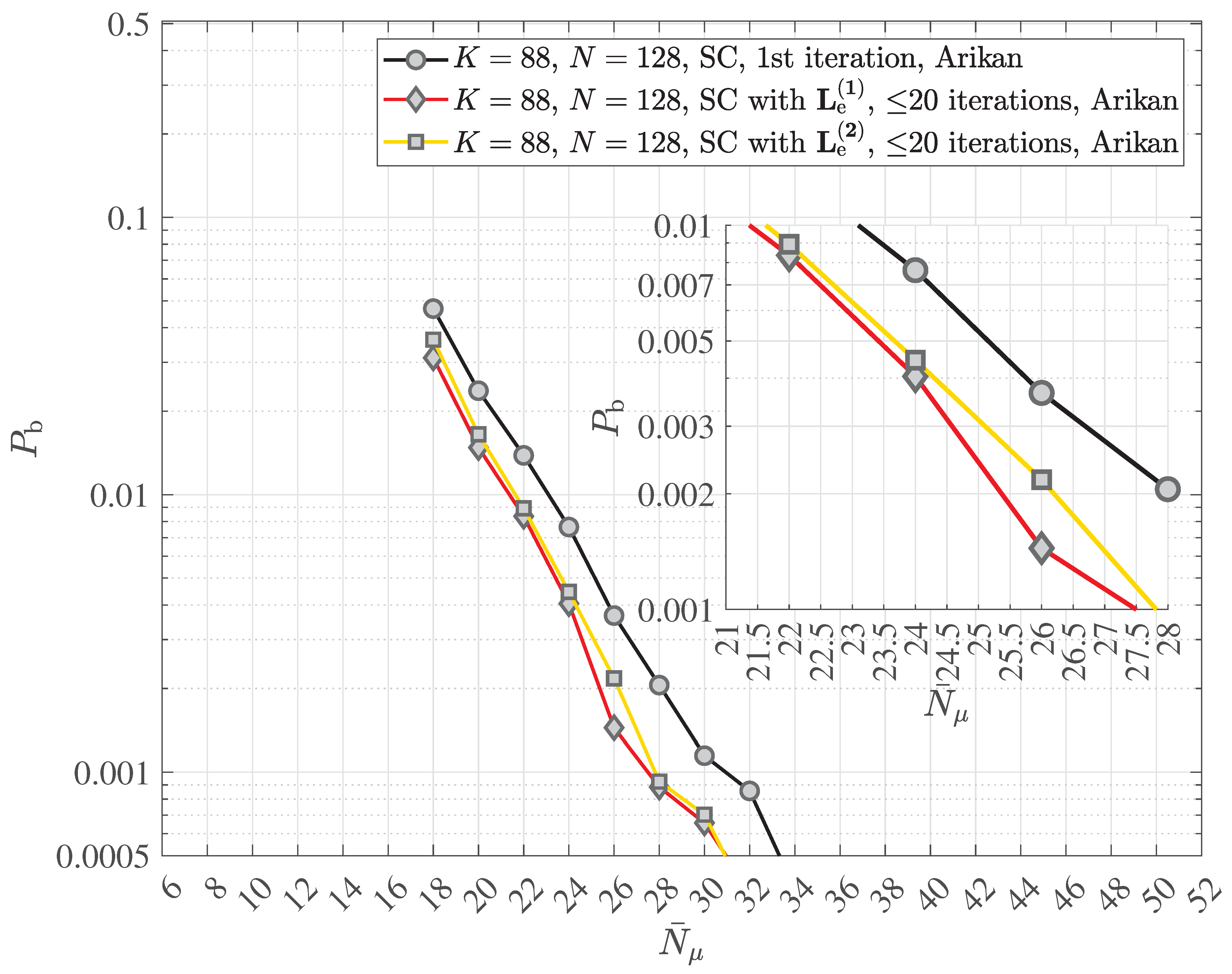
Figure 28.
Detail of simulation results of the block error ratio (BLER) performance versus the average number of signal photons per message bit with the average number of thermal photons equal to 0 for the transmission via the multipath quantum channel CIR#5 when turbo equalization with at most 20 iterations is taken into account, alternatively using the extrinsic soft output vector of (92), denoted by in the legend of this Figure 28, and according to (93), denoted by in the legend of this Figure 28; the polar code decoding is accomplished with the original SC decoder proposed by Arikan, hence, no CRC bits are required for the decoding but only for the termination control of the turbo equalization; the original Arikan polar code is applied with the generator matrix of (72) and the polar sequence generated by applying Arikan’s Bhattacharyya parameter based approach, setting out from the binary erasure channel with erasure probability , code dimension , code length , code rate ; the code rate is explicitly included in ; block interleaving according to the illustration in Section 3.3 is deployed.
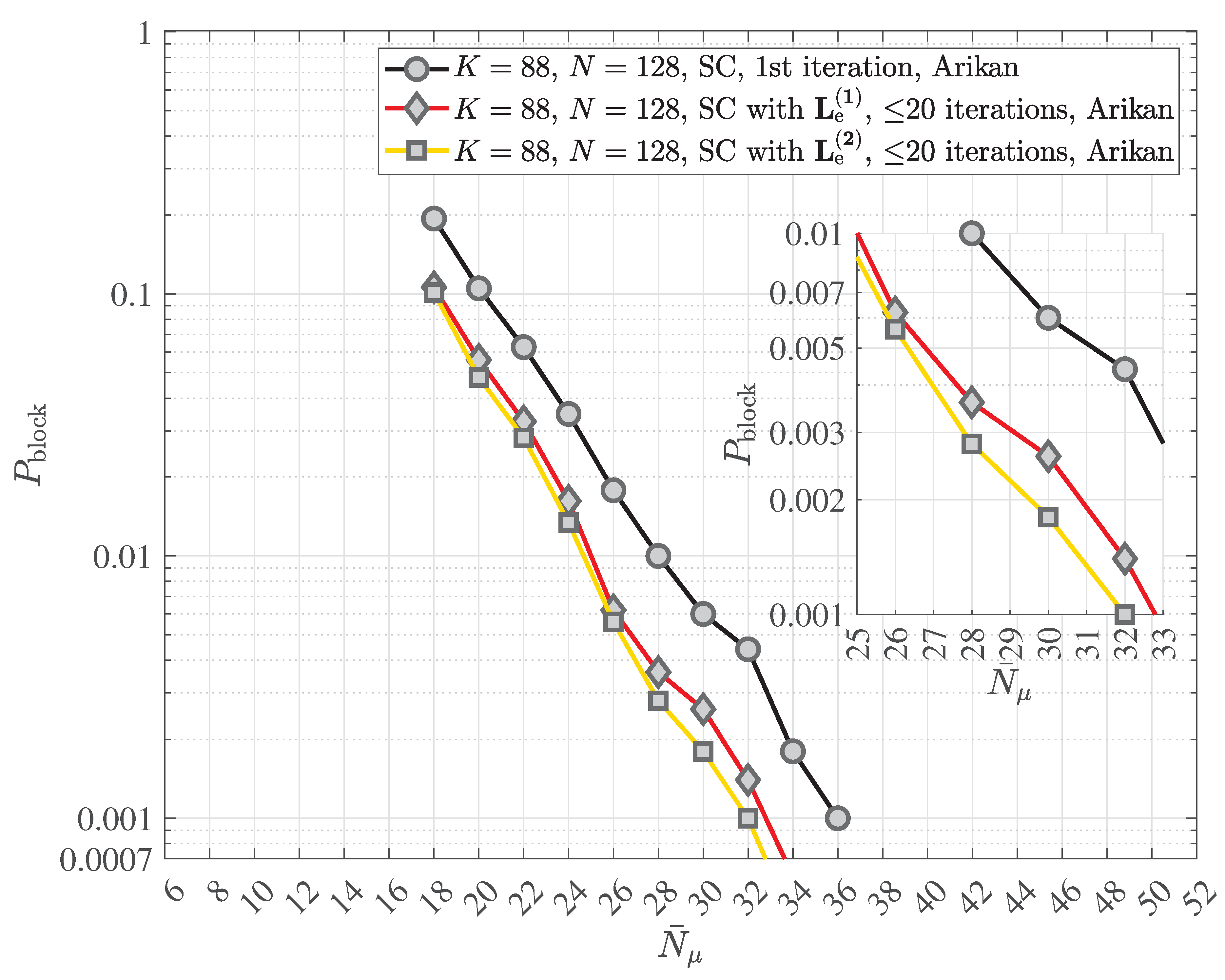
Figure 29 depitcs the average number of turbo equalization iterations versus the average number of signal photons per message bit required to obtain the simulation results shown in Figure 27 and Figure 28. In the considered scenario, on average, fewer than two turbo equalization iterations are sufficient to achieve the coded BER of less than , cf. Figure 27, and, correspondingly, the BLER of less than , cf. Figure 28, which occurs for .
As expected, the real nonnegative scaling factor of (94) varies adaptively. Moreover, the real nonnegative scaling factor depends on the average number of signal photons per message bit required to obtain the simulation results shown in Figure 27 and Figure 28. In the case of , the average real nonnegative scaling factor assumes values around or below .
Figure 29.
Average number of turbo equalization iterations versus the average number of signal photons per message bit required to obtain the simulation results shown in Figure 27 and Figure 28; the error bars indicate the estimated standard deviation in both the positive and negative directions.
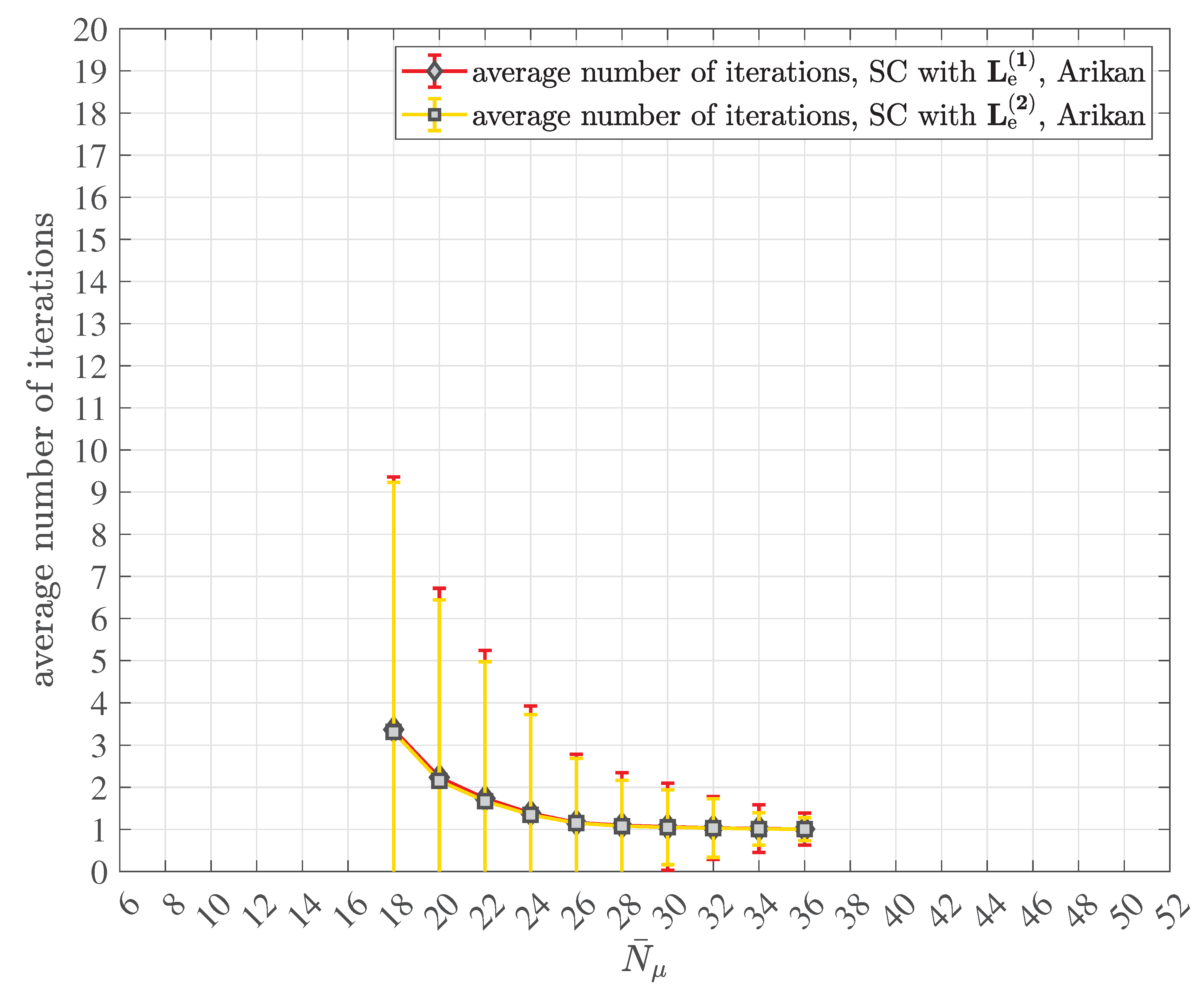
Figure 30.
Real nonnegative scaling factor of (94) versus the average number of signal photons per message bit required to obtain the simulation results shown in Figure 27 and Figure 28; the error bars indicate the estimated standard deviation in both the positive and negative directions.
Figure 31 illustrates the detail of simulation results of the BLER performance versus the average number of signal photons per message bit with the average number of thermal photons equal to 0 for the transmission via the multipath quantum channel CIR#4 when turbo equalization with at most 16 iterations is taken into account. In the case of curves labelled by “Arikan”, the polar code decoding is accomplished with the original SC decoder proposed by Arikan [39] or the soft cancellation (SCAN) decoder introduced by Fayyaz and Barry [50], hence, no CRC bits are required for the decoding. However, the CRC bits are used for the termination control of the turbo equalization. The original Arikan polar code was applied with the generator matrix of (72) and the polar sequence generated by applying Arikan’s Bhattacharyya parameter based approach, setting out from the binary erasure channel with erasure probability equal to . In the case of the curve labelled by “5G Polar Code”, the 3GPP 5G/NR polar code with the generator matrix of (71) and the polar sequence of [41][Table 5.3.1.2-1, pp. 17-19] was used with 24 CRC bits generated with polynomial “24C”. The code dimension K is equal to 64, the code length N is equal to 128 and the code rate is equal to , i.e. . The polar code decoding is accomplished with the CA-SCL decoder with the list length L equal to 8. In all cases, the code rate is explicitly included in . Block interleaving according to the illustration in Section 3.3 was deployed.
Figure 31.
Detail of simulation results of the block error ratio (BLER) performance versus the average number of signal photons per message bit with the average number of thermal photons equal to 0 for the transmission via the multipath quantum channel CIR#4 when turbo equalization with at most 16 iterations is taken into account; in the case of curves labelled by “Arikan”, the polar code decoding is accomplished with the original SC decoder proposed by Arikan [39] or the soft cancellation (SCAN) decoder introduced by Fayyaz and Barry [50], hence, no CRC bits are required for the decoding but only for the termination control of the turbo equalization; the original Arikan polar code was applied with the generator matrix of (72) and the polar sequence generated by applying Arikan’s Bhattacharyya parameter based approach, setting out from the binary erasure channel with erasure probability ; in the case of the curve labelled by “5G Polar Code”, the 3GPP 5G/NR polar code with the generator matrix of (71) and the polar sequence of [41][Table 5.3.1.2-1, pp. 17-19] is used with 24 CRC bits generated with polynomial “24C”; code dimension , code length , code rate ; the polar code decoding is accomplished with the CA-SCL decoder with the list length ; the code rate is explicitly included in ; block interleaving according to the illustration in Section 3.3 is deployed.
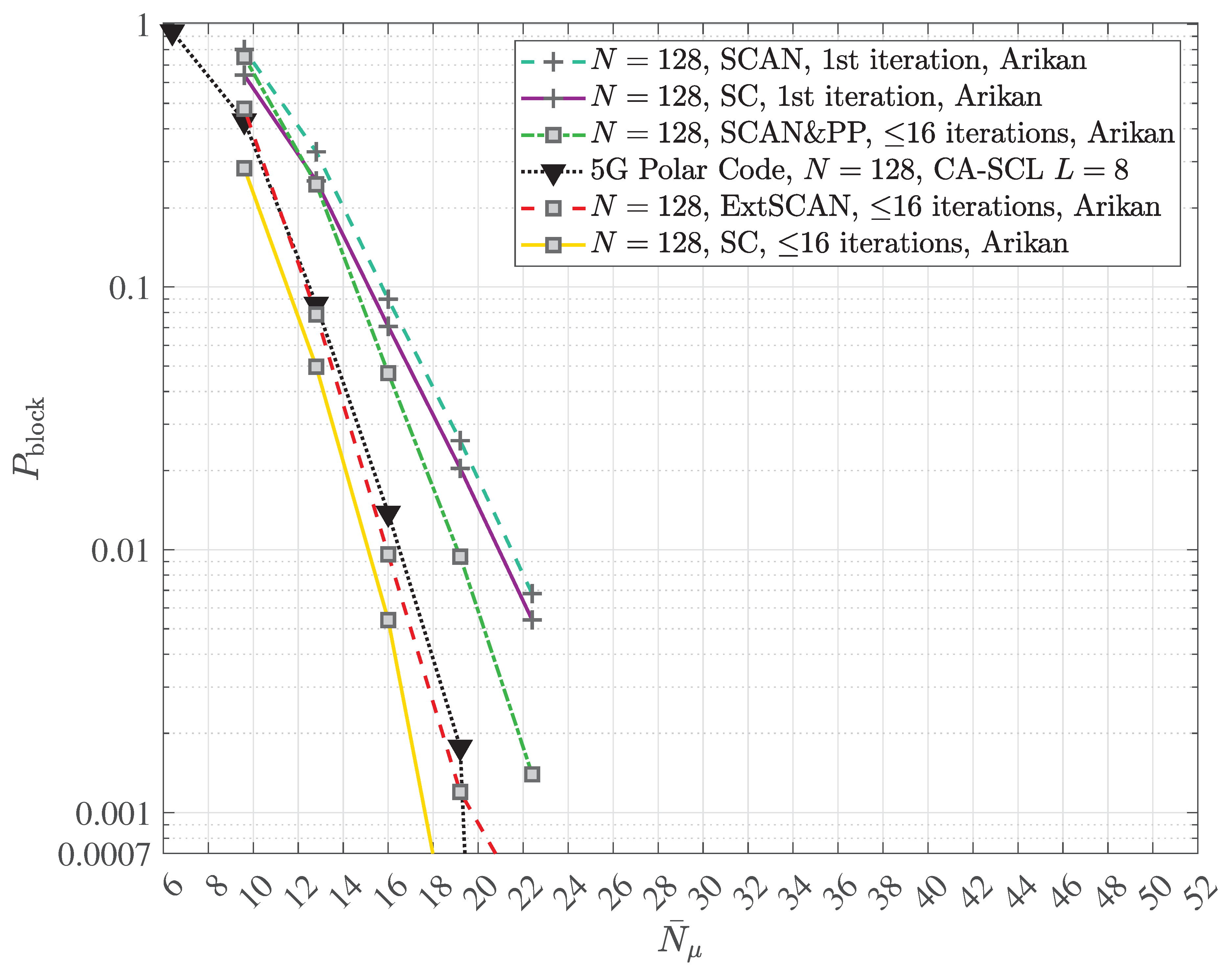
In Figure 31 “SCAN&PP” (SCAN and post processing) refers to the application of the SCAN decoder combined with the generation of the extrinsic soft output vector of (92). In the case of “ExtSCAN”, the extrinsic soft output vector is generated natively by the SCAN decoder as described in [50]. As expected, the BLER decreases monotonically with increasing for a given value of . Remarkably, the BLER after at most 16 turbo equalization iterations is always lower than in the case of a single pass. The SC decoder always provides an improved performance over the SCAN decoder. Furthermore, turbo equalization is capable of outperforming the 5G/NR polar code scheme using the CA-SCL decoder with the list length L equal to 8. In order to obtain the BLER , the required average number of signal photons is lower than 12.
Finally, Figure 32 shows the average number of turbo equalization iterations versus the average number of signal photons per message bit required to obtain the simulation results labelled by “, SC, iterations, Arikan” depicted in Figure 31. On average fewer than 5 turbo equalization iterations are required for .
Figure 32.
Average number of turbo equalization iterations versus the average number of signal photons per message bit required to obtain the simulation results labelled by “, SC, iterations, Arikan”, shown in Figure 31; the error bars indicate the estimated standard deviation in both the positive and negative directions.

Figure 33 and Figure 34 depict the details of simulation results of the coded BER performance, respectively, the BLER performance versus the average number of signal photons per message bit with the average number of thermal photons as the curve parameter for the transmission via the multipath quantum channel CIR#4, cf. the Figure 19 and Figure 20, when turbo equalization with at most 16 iterations is taken into account and the 3GPP 5G/NR polar code with the generator matrix of (71) associated with the polar sequence of [41][Table 5.3.1.2-1, pp. 17-19] is used. Figure 35 and Figure 36 depict the details of simulation results of the coded BER performance, respectively, the BLER performance versus the average number of signal photons per message bit with the average number of thermal photons as the curve parameter for the transmission via the multipath quantum channel CIR#4, cf. the Figure 19 and Figure 20, when turbo equalization with at most 16 iterations is taken into account and the Arikan-style polar code with the generator matrix of (72) associated with the polar sequence generated by Arikan’s Bhattacharyya parameter based approach, setting out from the binary erasure channel with erasure probability equal to , is used.
Figure 33.
Detail of simulation results of the coded bit error ratio (BER) performance versus the average number of signal photons per message bit with the average number of thermal photons as the curve parameter for the transmission via the multipath quantum channel CIR#4, cf. Figure 19, when turbo equalization with at most 16 iterations is taken into account; log-MAP quantum data detection is applied; the 3GPP 5G/NR polar code with the generator matrix of (71) and the polar sequence of [41][Table 5.3.1.2-1, pp. 17-19] is used; 24 CRC bits generated with polynomial “24C” are used; the polar code decoding is accomplished with the SC decoder, hence, CRC bits are not processed by the SC decoder; the code length N is 512; three choices of the code dimension, (—■—), (- - -▴- - -) and (- · -★- · -), leading to the three code rates (—■—), (- - -▴- - -) and (- · -★- · -) are considered; the code rate is explicitly included in ; interleaving is deployed.
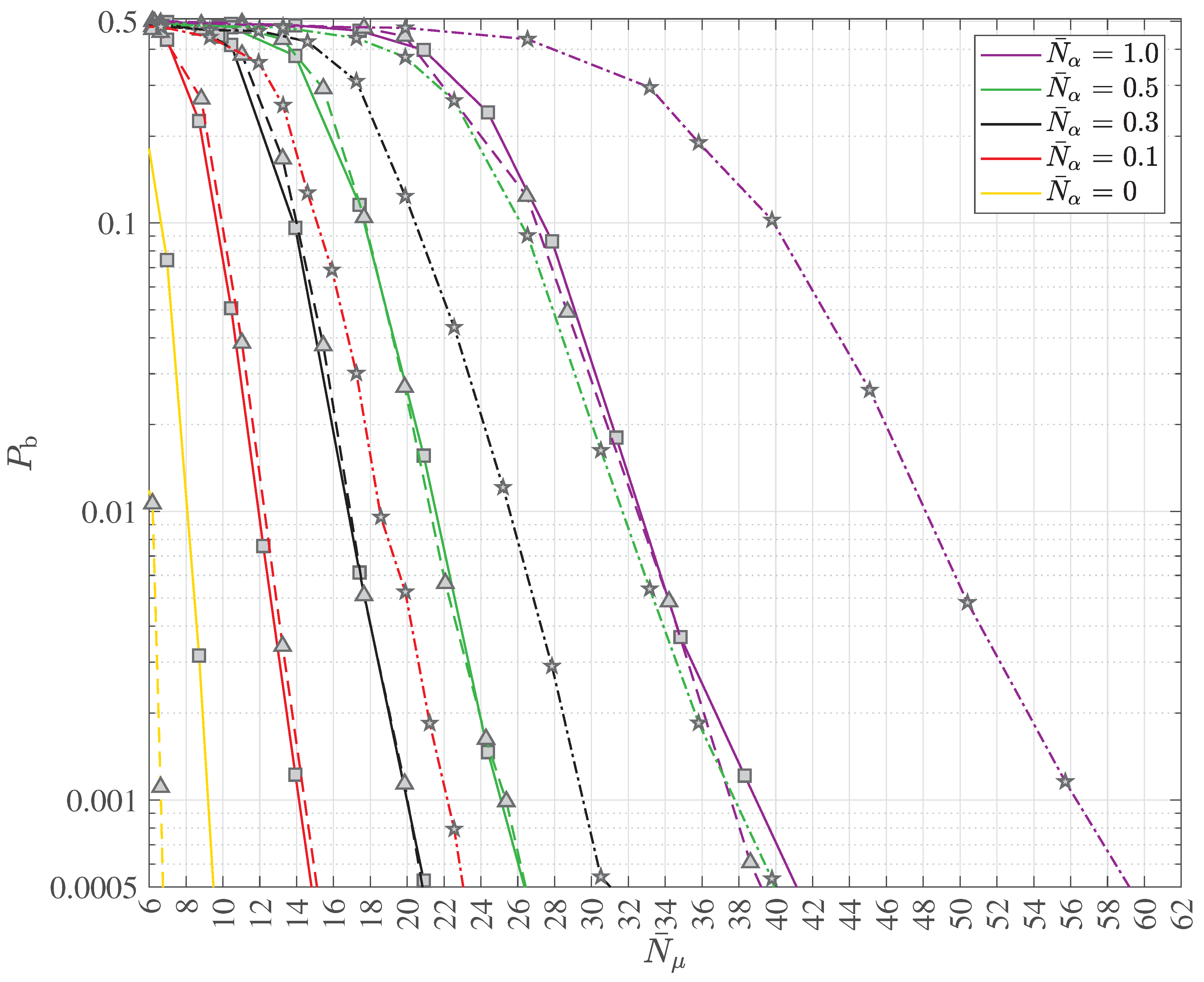
Figure 34.
Detail of simulation results of the block error ratio (BLER) performance versus the average number of signal photons per message bit with the average number of thermal photons as the curve parameter for the transmission via the multipath quantum channel CIR#4, cf. Figure 20, when turbo equalization with at most 16 iterations is taken into account; log-MAP quantum data detection is applied; the 3GPP 5G/NR polar code with the generator matrix of (71) and the polar sequence of [41][Table 5.3.1.2-1, pp. 17-19] is used; 24 CRC bits generated with polynomial “24C” are used; the polar code decoding is accomplished with the SC decoder, hence, CRC bits are not processed by the SC decoder; the code length N is 512; three choices of the code dimension, (—■—), (- - -▴- - -) and (- · -★- · -), leading to the three code rates (—■—), (- - -▴- - -) and (- · -★- · -) are considered; the code rate is explicitly included in ; interleaving is deployed.
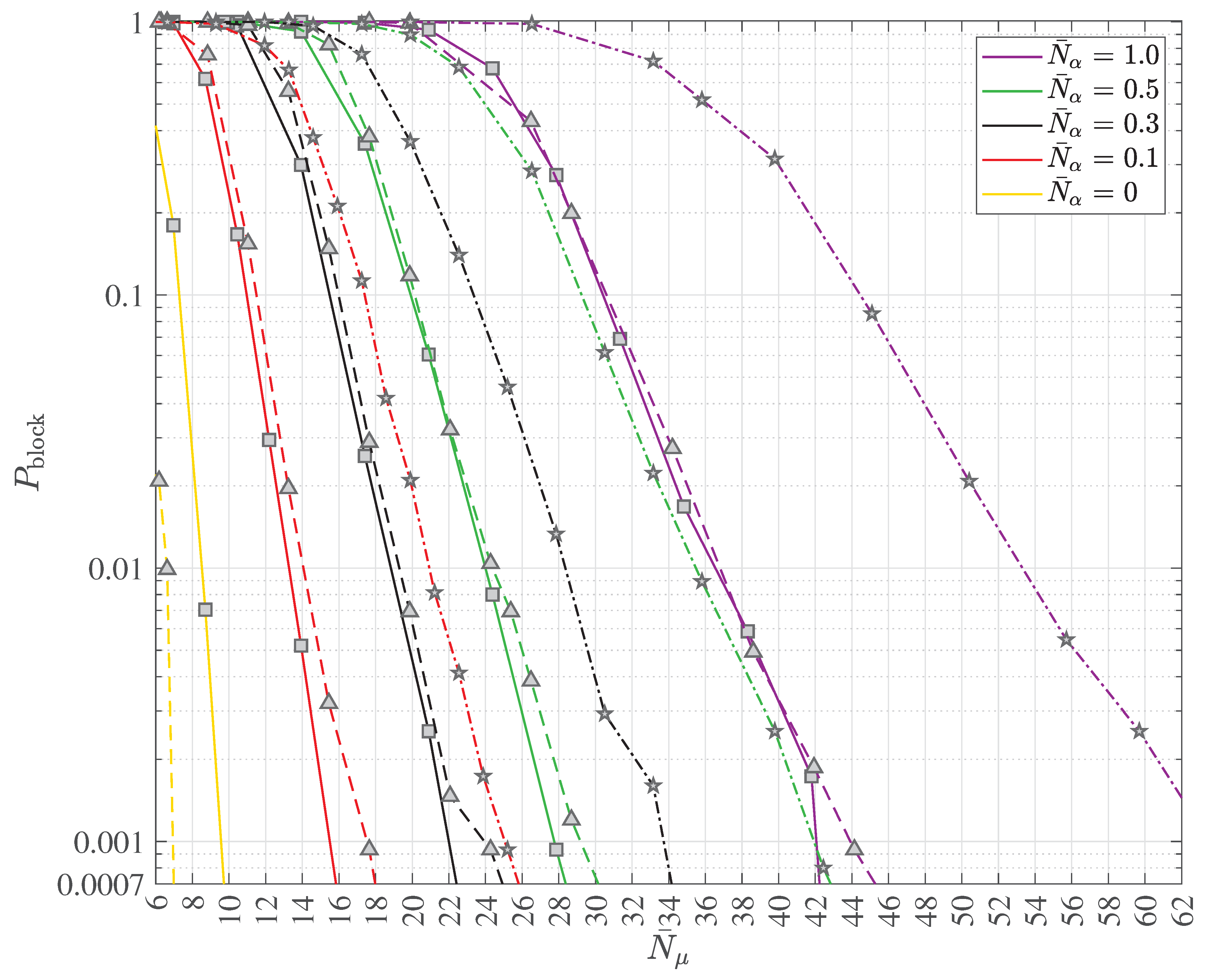
Figure 35.
Detail of simulation results of the coded bit error ratio (BER) performance versus the average number of signal photons per message bit with the average number of thermal photons as the curve parameter for the transmission via the multipath quantum channel CIR#4, cf. Figure 19, when turbo equalization with at most 16 iterations is taken into account; log-MAP quantum data detection is applied; the Arikan-style polar code with the generator matrix of (72) and the associated polar sequence generated by Arikan’s Bhattacharyya parameter based approach setting out from the binary erasure channel with erasure probability is used; 24 CRC bits generated with polynomial “24C” are used; the polar code decoding is accomplished with the SC decoder, hence, CRC bits are not processed by the SC decoder; the code length N is 512; three choices of the code dimension, (—■—), (- - -▴- - -) and (- · -★- · -), leading to the three code rates (—■—), (- - -▴- - -) and (- · -★- · -) are considered; the code rate is explicitly included in ; interleaving is deployed.
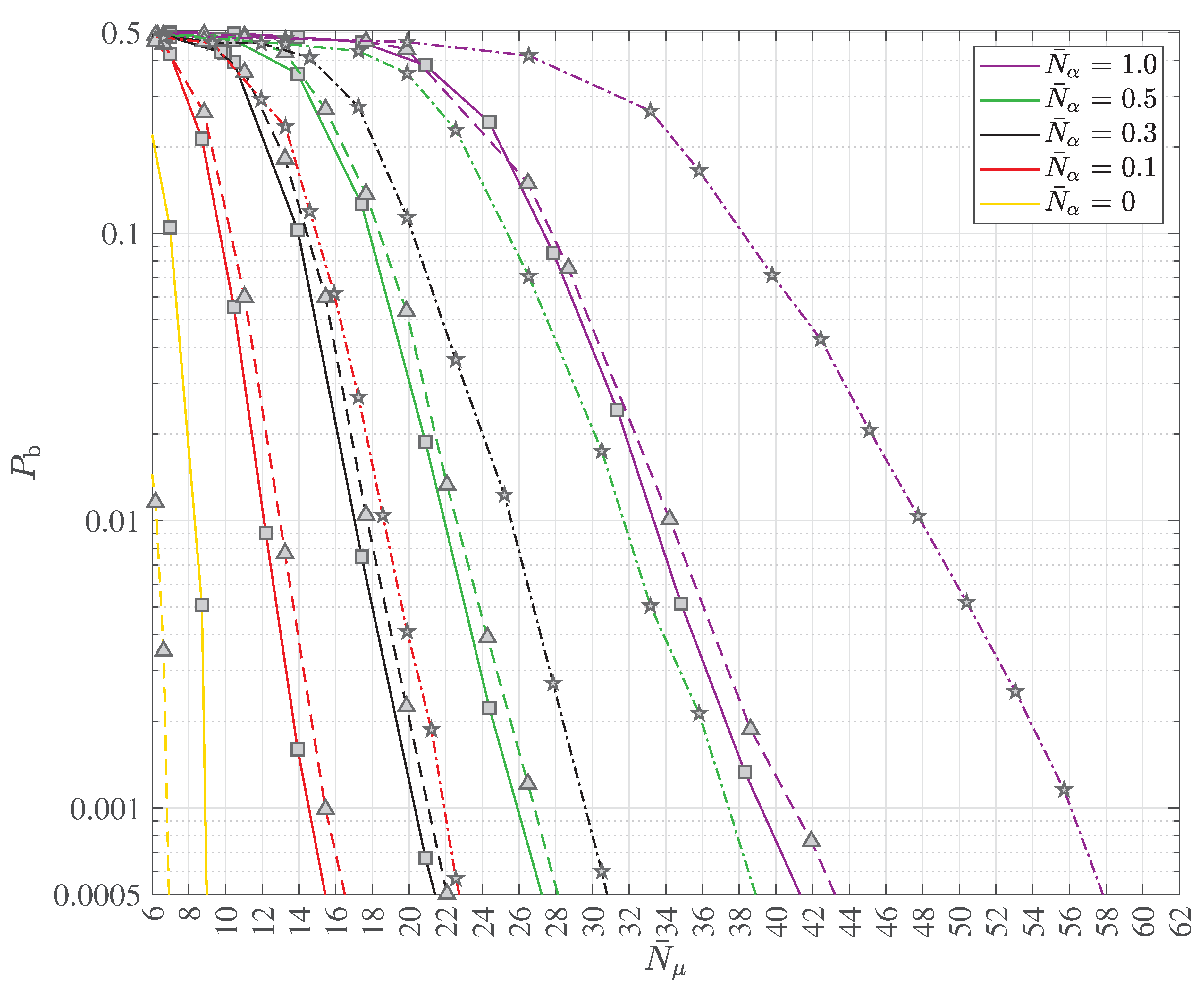
Figure 36.
Detail of simulation results of the block error ratio (BLER) performance versus the average number of signal photons per message bit with the average number of thermal photons as the curve parameter for the transmission via the multipath quantum channel CIR#4, cf. Figure 20, when turbo equalization with at most 16 iterations is taken into account; log-MAP quantum data detection is applied; the Arikan-style polar code with the generator matrix of (72) and the associated polar sequence generated by Arikan’s Bhattacharyya parameter based approach setting out from the binary erasure channel with erasure probability is used; 24 CRC bits generated with polynomial “24C” are used; the polar code decoding is accomplished with the SC decoder, hence, CRC bits are not processed by the SC decoder; the code length N is 512; three choices of the code dimension, (—■—), (- - -▴- - -) and (- · -★- · -), leading to the three code rates (—■—), (- - -▴- - -) and (- · -★- · -) are considered; the code rate is explicitly included in ; interleaving is deployed.
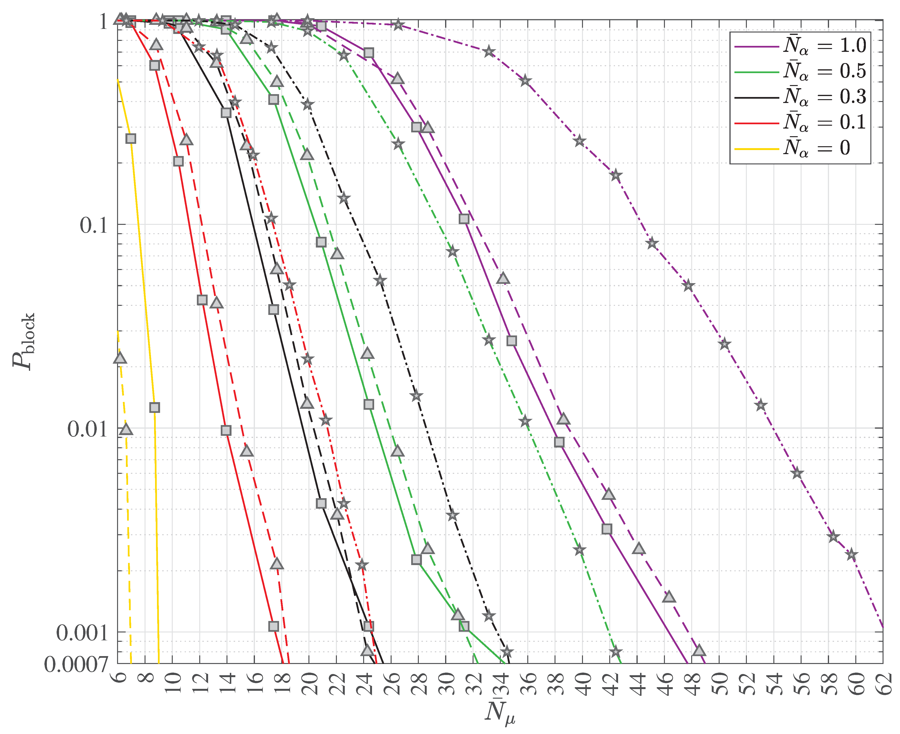
In all shown cases, log-MAP quantum data detection is applied. 24 CRC bits generated with polynomial “24C” are used. The polar code decoding is accomplished with the SC decoder, hence, CRC bits are not processed by the SC decoder. The code length N is equal to 512. Furthermore, three choices of the code dimension, K equal to 171 (—■—), K equal to 256 (- - -▴- - -) and K equal to 410 (- · -★- · -), leading to the three code rates equal to , i.e. (—■—), equal to , i.e. (- - -▴- - -) and equal to , i.e. (- · -★- · -) are considered. Of course, the code rate is explicitly included in . In addition, interleaving according to the illustration in Section 3.3 was deployed. Both the coded BER , respectively the BLER , decreases monotonically with increasing for a given value of . Furthermore, the coded BER , respectively the BLER , increases with increasing thermal noise, i.e. with increasing , for a given value of . Comparing the Figure 33 and Figure 19 as well as Figure 34 and Figure 20, the beneficial effect of turbo equalization on the respective performance becomes obvious. For instance, in the case of equal to , i.e. , no errors were measured in the simulations. Table 6 summarizes the estimated average number of signal photons required to obtain equal to and equal to associated with the results shown in Figure 19, Figure 20, Figure 21, Figure 22, Figure 33, Figure 34, Figure 35 and Figure 36.
Table 6.
Estimated average number of signal photons per message bit required to obtain and associated with the results shown in Figure 19, Figure 20, Figure 21, Figure 32, Figure 33, Figure 34, Figure 35 and Figure 36,
| polar code | iteration | |||||||
|---|---|---|---|---|---|---|---|---|
| BER | 3GPP 5G/NR | 1 | ||||||
| BER | 3GPP 5G/NR | 16 | ||||||
| BER | Arikan | 1 | ||||||
| BER | Arikan | 16 | ||||||
| BER | 3GPP 5G/NR | 1 | ||||||
| BER | 3GPP 5G/NR | 16 | ||||||
| BER | Arikan | 1 | ||||||
| BER | Arikan | 16 | ||||||
| BER | 3GPP 5G/NR | 1 | ||||||
| BER | 3GPP 5G/NR | 16 | error-free | |||||
| BER | Arikan | 1 | ||||||
| BER | Arikan | 16 | error-free | |||||
| BLER | 3GPP 5G/NR | 1 | ||||||
| BLER | 3GPP 5G/NR | 16 | ||||||
| BLER | Arikan | 1 | ||||||
| BLER | Arikan | 16 | ||||||
| BLER | 3GPP 5G/NR | 1 | ||||||
| BLER | 3GPP 5G/NR | 16 | ||||||
| BLER | Arikan | 1 | ||||||
| BLER | Arikan | 16 | ||||||
| BLER | 3GPP 5G/NR | 1 | ||||||
| BLER | 3GPP 5G/NR | 16 | error-free | |||||
| BLER | Arikan | 1 | ||||||
| BLER | Arikan | 16 | error-free |
Extrinsic information transfer (EXIT) charts [58] have been widely regarded as a valuable tool for analyzing iterative reception processes. Building on this notion, we adopt a similar approach, but without attempting to separate the intrinsic information represented by the photon count vector in (28) from the pure extrinsic information generated by the quantum data detector in Figure 10. Let denote the conditional probability density function (pdf) of the ith component of the input vector , cf. (81), given the transmitted codebit , . Similarly, let denote the conditional pdf of the ith component of the extrinsic soft output vector denoted by , given the transmitted codebit , . The conditional pdfs and are approximated via histograms obtained from simulations.
Following [58, Eqs. (12) and (19), pp. 1728f.] and using these approximated conditional pdfs and , we estimate the mutual information between the transmitted codebits , , supposed to assume the values 0 and 1 with the same a-priori probability , and the components of the input vector , cf. (81), as given by
as well as the mutual information between the transmitted codebits , , and the components of the extrinsic soft output vector denoted by , given by
for each iteration of the turbo equalization.
Figure 37 shows simulation results of the estimated mutual information , cf. (98), versus the estimated mutual information , cf. (99), in the case of six different values of . Like in the original EXIT charts, each horizontal line refers to a distinct iteration of the turbo equalization, the leftmost line associated with a particular referring to the respective first iteration. The multipath quantum channel CIR#5 is considered and the average number of thermal photons is equal to 0. The Arikan-style polar code with the generator matrix of (71) and the associated polar sequence generated by Arikan’s Bhattacharyya parameter based approach setting out from the binary erasure channel with erasure probability equal to is used. As usual for the simulations discussed in this Section 4.4, 24 CRC bits generated with polynomial “24C” are applied for the termination control of the turbo equalization. The code dimension K is equal to 88 and the code length N is equal to 128, yielding the code rate equal to , i.e. . SC decoding and log-MAP quantum data detection are used. Also, block interleaving according to the illustration in Section 3.3 is deployed.
Figure 37.
Simulation results of the estimated mutual information , cf. (96), versus the estimated mutual information , cf (97); each horizontal line refers to a distinct iteration of the turbo equalization; the multipath quantum channel CIR#5 is considered and the average number of thermal photons is equal to 0; the Arikan-style polar code with the generator matrix of (72) and the associated polar sequence generated by Arikan’s Bhattacharyya parameter based approach setting out from the binary erasure channel with erasure probability is used; 24 CRC bits generated with polynomial “24C” are applied for the termination control of the turbo equalization; code dimension , code length , code rate ; log-MAP quantum data detection and SC decoding are used; block interleaving according to the illustration in Section 3.3 is deployed.
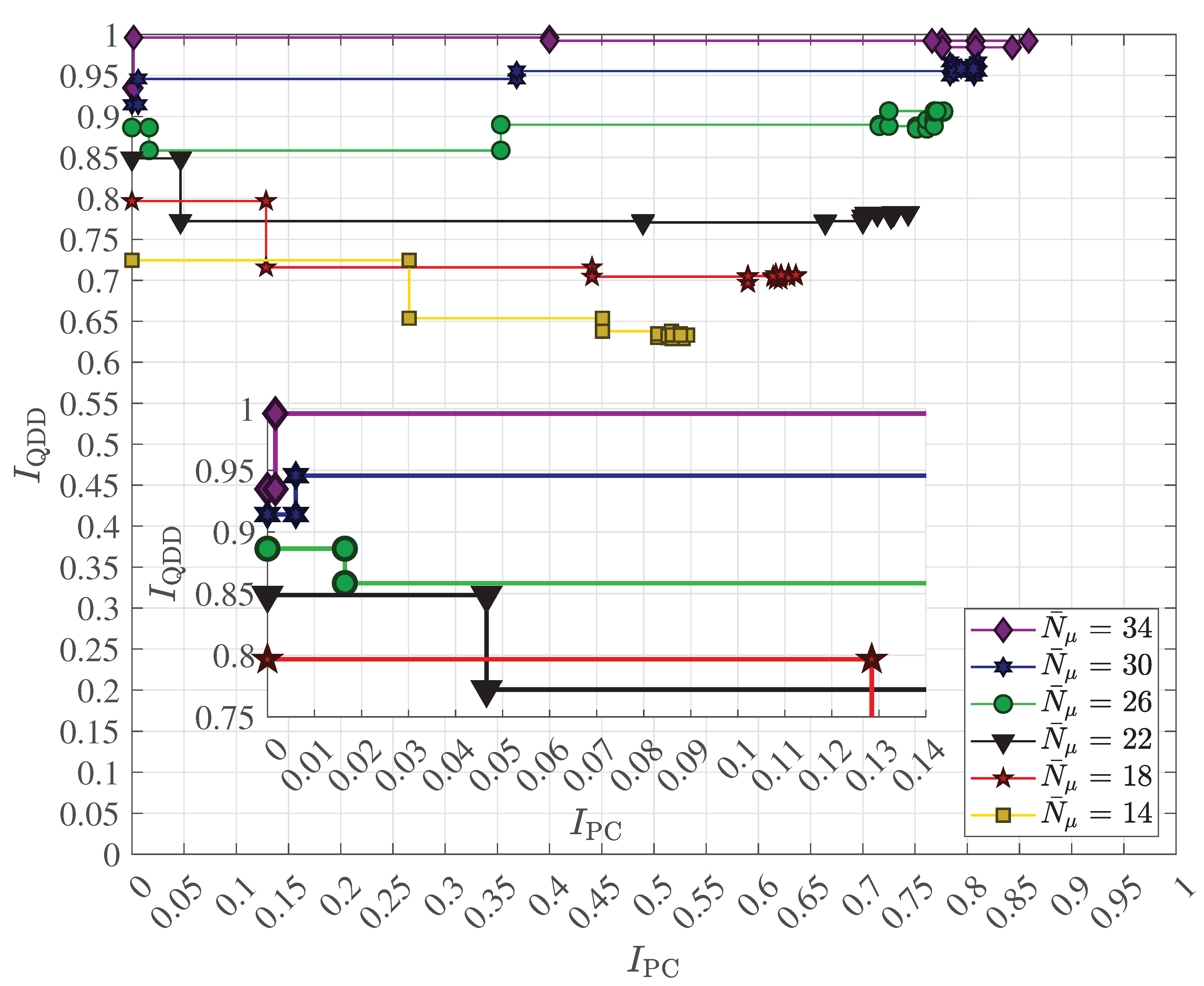
Obviously increases from 0 to positive values during the turbo equalization process. The maximum increase of is greater for high values of than for low values of . Furthermore, after about the first three iterations, the change of depicted in Figure 37 diminishes when further iterations occur. Remarkably, sets out from high values, greater than in Figure 37, and the change of during the turbo equalization is rather small. Similar observations for turbo equalization applied in other transmission schemes are found in e.g. [59, Fig. 3, p. 2; Fig. 6, p. 4]. Also, it seems that improvements of are only possible for high values of , higher than 22 in Figure 37.
5. Conclusions
Future wireless communication systems, such as 6G and beyond, will operate at carrier frequencies above and will therefore increasingly need to employ optical transmission technologies. Motivated by this certainty, the authors have explored concepts in wireless quantum optical communications and demonstrated that such concepts are well-suited for implementation within the physical layer. Of particular interest is the suitability of sophisticated channel coding, especially polar coding, in combination with such wireless quantum optical communication concepts.
To improve clarity and provide a foundation for the later discussions on polar codes, the authors first presented a brief overview of optimum soft output quantum data detection, a novel near-optimum soft output quantum data detection based on Kohonen maps, introduced here for the first time, and a likewise novel suboptimum soft output quantum data detection scheme using state reduction, also introduced here for the first time. Following a concise explanation of the fundamental differences between Arikan-style polar codes and those used in 3GPP 5G/NR, the authors describe a novel design method for generating the polar sequence, introduced here for the first time. They also discuss turbo equalization, including a detailed and explicit method for computing the soft output vector associated with the codebits as well as the novel fully analytical generation of the extrinsic soft output vector , without resorting to any time-consuming optimization procedures.
Finally, the achievable transmission quality when using polar codes in combination with wireless quantum optical communication concepts is thoroughly investigated and discussed in terms of BER and BLER in numerous scenarios. The studies consistently demonstrate the feasibility of the mentioned combination and confirm the long-term viability of suitably designed systems.
The authors point out that the laser as a light source can also be replaced by thermal light sources that produce chaotic light. The explanations presented here can be readily adapted. The authors intend to demonstrate this elsewhere.
The authors also make no secret of the fact that topics often associated with quantum communications, such as entanglement and quantum teleportation, were not explicitly considered. The above explanations have shown that these aspects of quantum physics are not fundamental prerequisites for the proper functioning of the considered concept of wireless quantum optical communication technology, and can therefore be added later as needed.
Furthermore, the authors did not address so-called “nonclassical” light sources, which, for example, produce squeezed light through the use of nonlinear optics. The authors are concerned with presenting a simple, robust, and yet functional technology. Due to the effort involved in generating squeezed light alone, it is by no means supporting this asset.
Based on the experience gathered over several years, some of which is presented here, the authors are confident that future analyses will help turn their conviction into a broadly shared certainty among many engineers. Therefore, the authors are convinced that the path they have taken will lead to both robust and economically viable solutions.
References
- Jung, P.; Dini, K. : Frequency dependence of the ohmic resistance in the sixth generation terahertz band. Proceedings of the IEEE International Mediterranean Conference on Communications and Networking (MeditCom), Nice, France, 2025.
- Rietschel, H.; Esdorn, H. : Raumklimatechnik — Band 1: Grundlagen. Sixteenth edition, Heidelberg: Springer, 2008.
- Deutsches Institut für Normung (DIN): Strahlungsphysik im optischen Bereich und Lichttechnik; Benennung der Wellenlängenbereiche. DIN 5031 Part 7, January 1984.
- Arute, F. et al. Quantum supremacy using a programmable superconducting processor. Nature 2019, 574, 505–511. [Google Scholar] [CrossRef] [PubMed]
- Cariolaro, G. : Quantum communications. Cham: Springer, 2015.
- Helstrom, C.W.; Liu, J.W.S.; Gordon, J.P. Quantum-mechanical communication theor. Proceedings of the IEEE 1970, 58, 1578–1589. [Google Scholar] [CrossRef]
- Jung, P. : Einführung in die Quantenkommunikation. Düren: Shaker, 2022.
- Jung, P. : Advanced mobile communications — sophisticated channel codes. Berlin: Walter de Gruyter, 2024.
- Helstrom, C.W. : Quantum detection and estimation theory. New York: Academic Press, 1976.
- ISO/IEC/IEEE 8802-11: Telecommunications and information exchange between systems — specific requirements for local and metropolitan area networks — part 11: Wireless LAN medium access control (MAC) and physical layer (PHY) specifications. Third edition, July 2022.
- IEEE Std 802.11bb-2023: Telecommunications and information exchange between systems — local and metropolitan area networks — specific requirements — part 11: Wireless LAN medium access control (MAC) and physical layer (PHY) specifications — amendment 6: Light communications. June 2023.
- Jung, P.; Bruck, G.H. Transmitter and receiver for transceiving optical signals. European Patent Specification EP 2 478 653 B1 (filed 17 Sept. 2009), 23 July 2014.f.
- Shehata, M.; Wang, Y.; He, J.; Kandeepan, S.; Wang, K. : Optical and terahertz wireless technologies: The race to 6G communications. IEEE Wireless Communications, vol. 30 (2023) no. 5, pp. 10-18.
- Schlosshauer, M. : Decoherence and the quantum-to-classical transition. Berlin: Springer, 2007.
- Buchleitner, A.; Viviescas, C.; Tiersch, M. (Eds.): Entanglement and decoherence — foundations and modern trends. Lecture Notes in Physics 768, Berlin: Springer, 2009.
- Joos, E.; Zeh, H.D:; Kiefer, C.; Giulini, D.; Kupsch, J.; Stamatescu, I.-O.: Decoherence and the appearance of a classical world in quantum theory. Second edition, Berlin: Springer, 2010.
- Jung, P. : Advanced mobile communications — inner physical layer transceiver. Berlin: Walter de Gruyter, 2024.
- Bello, P.A. Characterization of randomly time-variant linear channels. IEEE Transactions on Communications Systems 1963, 11, 360–393. [Google Scholar] [CrossRef]
- Jung, P.; Bruck, G.H. Wireless quantum optical communications with uncorrelated scattering multipath reception. IET Electronics Letters 2024, 60, 1–3. [Google Scholar] [CrossRef]
- Jung, P.; Dini, K.; Almujahed, H. : Applying turbo codes to wireless quantum optical communications via multipath channels causing intersymbol interference. Proceedings of the 2025 IEEE International Conference on Quantum Communications, Networking, and Computing (QCNC), Nara, Japan, pp. 24-31, 2025.
- Jung, P.; Dini, K.; Almujahed, H. : Polar encoded wireless quantum optical communications with intersymbol interference caused by multipath propagation. Proceedings of the 2025 IEEE International Conference on Communications (ICC), Montreal, Canada, 2025.
- Abdel Rehim, F.; Jung, P. : Kohonen maps based near optimum sequence detection. Proceedings of the IEEE International Mediterranean Conference on Communications and Networking (MeditCom), Nice, France, 2025.
- Dini, K.; Jung, P.; Almujahed, H. : Connecting polar codes and 6G short range wireless quantum optical communications. Proceedings of the IEEE International Mediterranean Conference on Communications and Networking (MeditCom), Nice, France, 2025.
- Gradshteyn, I.S.; Ryzhik, I.M. : Table of integrals, series, and products. Eighth edition, Amsterdam: Elsevier, 2015.
- Schwabl, F. : Quantenmechanik — eine Einführung, Band 1. Seventh edition, Berlin: Springer, 2007.
- Hoversten, E.V.; Harger, R.O.; Halme, S.J. : Communication theory for the turbulent atmosphere. Proceedings of the IEEE, vol. 58 (1970) no. 10, pp. 1626-1650.
- Sauer-Greff, W. : Optimale und suboptimale Empfänger für verzerrte und gestörte Datensignale unter besonderer Berücksichtigung der aufwandsreduzierten Detektion mittels M-Algorithmus. Doctoral Dissertation, FB Elektrotechnik, Universität Kaiserslautern, Germany, 1989. [Google Scholar]
- Forney, D.G. : Maximum-likelihood sequence estimation of digital sequences in the presence of intersymbol interference. IEEE Transactions on Information Theory, vol. IT-18 (1972) no. 3, pp. 363-378.
- Gerry, C.; Knight, P. : Introductory quantum optics. Cambridge: Cambridge University Press, 2005.
- Shih, Y. : An introduction to quantum optics. Boca Raton: CRC Press, 2021.
- Takahashi, H. : Information theory of quantum-mechanical channels. In: Advances in Communication Systems, vol. 1 (1965), pp. 227-310.
- Henze, N. : Stochastik für Einsteiger. Eleventh edition, Wiesbaden: Springer, 2017.
- Jung, P. : Einführung in die Quanteninformationstheorie. Düren: Shaker, 2022.
- Kolmogorov, A.N. : Foundations of the theory of probability. Mineola: Dover, 2018.
- Jung, P. : Analyse und Entwurf digitaler Mobilfunksysteme. Stuttgart: Teubner, 1997.
- Bahl, L.R., Cocke, J., Jelinek, F., Raviv, J.: Optimal decoding of linear codes for minimizing symbol error rate. IEEE Transactions on Information Theory 1974, 20, 284–287. [CrossRef]
- Hagenauer, J. Source-controlled channel decoding. IEEE Transactions on Communications 1995, 43, 2449–2457. [Google Scholar] [CrossRef]
- Kohonen, T. : Self-organizing maps. Third edition, Berlin: Springer, 2001.
- Arikan, E. Channel polarization: A method for constructing capacity-achieving codes for symmetric binary-input memoryless channels. IEEE Transactions on Information Theory 2009, 55, 3051–3073. [Google Scholar] [CrossRef]
- Plotkin, M. Binary codes with specified minimum distancE. IRE Transactions on Information Theory 1960, 6, 445–450. [Google Scholar] [CrossRef]
- 3GPP TS 38.212 V17.5.0 (2023-03): Multiplexing and channel coding. March 2023.
- Zhou, Y.; Li, R.; Zhang, H.; Luo, H.; Wang, J. : Polarization weight family methods for polar code construction. Proceedings of the 2018 IEEE 87th Vehicular Technology Conference (VTC Spring), Porto, Portugal, 2018.
- Mori, R.; Tanaka, T. : Performance and construction of polar codes on symmetric binary-input memoryless channels. Proceedings of the 2009 IEEE International Symposium on Information Theory, Seoul, South Korea, 2009.
- Hensel, K. : Über eine neue Begründung der Theorie der algebraischen Zahlen. Jahresbericht der Deutschen Mathematiker-Vereinigung 1897, 6, 83–88. [Google Scholar] [CrossRef]
- Hensel, K. : Zahlentheorie. Berlin: G.J. Göschen’sche Verlagshandlung G.m.b.H., 1913.
- Koblitz, N. : p-adic numbers, p-adic analysis, and zeta-functions. Second edition, New York: Springer, 1984.
- Douillard, C.; Jezequel, M.; Berrou, C.; Picart, A.; Didier, P. Iterative correction of intersymbol interference: Turbo-equalization. European Transactions on Telecommunications 1995, 6, 507–512. [Google Scholar] [CrossRef]
- Hagenauer, J. : Source-controlled channel decoding. Proceedings of the 1994 IEEE International Symposium on Information Theory, Trondheim, Norway, p. 165, 1994.
- Holma, H.; Toskala, A.; Nakamura, T. : 5G technology — 3GPP evolution to 5G-Advanced. Second edition, Chichester: Wiley, 2020.
- Fayyaz, U.U.; Barry, J. R: Low-complexity soft-output decoding of polar codes. IEEE Journal on Selected Areas in Communications 2014, 32, 958–966. [Google Scholar] [CrossRef]
- Jung, P. : Mobilkommunikation — anspruchsvolle Kanalcodes. Berlin: Walter de Gruyter, 2025.
- Hagenauer, J. : The turbo principle: Tutorial introduction and state of the art. Proceedings of the International Symposium on Turbo Codes and Related Topics, Brest, France, pp. 1-11, 1997.
- Berrou, C.; Glavieux, A.; Thitimajshima, P. : Near Shannon limit error-correcting coding and decoding: Turbo-codes (1). Proceedings of the IEEE International Conference on Communications (ICC’93), Geneva, Switzerland, pp. 1064-1070, 1993.
- Eltohamy, A.; Hofmann, C.A.; Knopp, A:; Korb, M.: Turbo receiver for short-block-length polar-coded direct-access satellite-IoT systems. Proceedings of the IEEE International Mediterranean Conference on Communications and Networking (MeditCom), Madrid, Spain, pp. 143-148, 2024.
- Jung, P. : Mobilkommunikation — innere physikalische Schicht. Berlin: Walter de Gruyter, 2025.
- Pätzold, M. : Mobile radio channels. Second edition, Chichester: Wiley, 2012.
- Failli, M. (chairman): Digital land mobile radio communications. European Cooperation in Science and Technology Action 207 (COST 207), Brussels/Luxemburg: ECSC-EEC-EAEC, 1989.
- ten Brink, S. Convergence behavior of iteratively decoded parallel concatenated codes. IEEE Transactions on Communications 2001, 49, 1727–1737. [Google Scholar] [CrossRef]
- Schorr, T.; Matuszak, M.; Sauer-Greff, W.; Urbansky, R. : LDPC code optimization for diversity reception and turbo equalization. Proceedings of the IEEE International Mediterranean Conference on Signal Processing Algorithms, Architectures, Arrangements, and Applications (SPA 2007), Poznan, Poland, pp. 63-68, 2007.
Disclaimer/Publisher’s Note: The statements, opinions and data contained in all publications are solely those of the individual author(s) and contributor(s) and not of MDPI and/or the editor(s). MDPI and/or the editor(s) disclaim responsibility for any injury to people or property resulting from any ideas, methods, instructions or products referred to in the content. |
© 2025 by the authors. Licensee MDPI, Basel, Switzerland. This article is an open access article distributed under the terms and conditions of the Creative Commons Attribution (CC BY) license (https://creativecommons.org/licenses/by/4.0/).
Copyright: This open access article is published under a Creative Commons CC BY 4.0 license, which permit the free download, distribution, and reuse, provided that the author and preprint are cited in any reuse.


