
Submitted:
17 August 2025
Posted:
18 August 2025
You are already at the latest version
Abstract
Background: Metabolic disorders such as obesity have increased globally in recent decades and are a major public health concern. Previous research suggests that herbicide exposures may contribute to metabolic dysfunction, but few studies have examined mixture effects of multiple herbicides on obesity at a population level.
Methods: Using county-level data from 2013 to 2018, we examined the associations between obesity rates and the application of 13 commonly applied herbicides in the U.S. We first conducted adjusted single-pollutant mixed effects models and then used quantile-based g-computation mixture modeling to assess combined herbicide mixture effects on county-level obesity rates. Models were adjusted for demographic and socioeconomic covariates and accounted for geographic clustering.
Results: Significant positive associations were identified between county-level obesity rates and applications of glyphosate, 2,4-D, atrazine, acetochlor, metolachlor, and several other herbicides in adjusted single-pollutant models. Glyphosate showed one of the strongest individual associations (β=0.29 per standard deviation increase, 95% CI: 0.21–0.36). Increases in herbicide mixture were significantly associated with higher obesity rates (Psi=0.71 per quantile exposure mixture, 95% CI: 0.65–0.76) from mixture modeling. Inclusion of significant interaction terms did not ap-preciably increase the mixture effect. Glyphosate, 2,4-D, metolachlor, dimethenamid-P, and glufosinate contributed most strongly to the weighted mixture effect. Mixture effects varied by rurality, with stronger associations observed in rural counties, particularly in micropolitan regions.
Conclusions: Our findings highlight the importance of considering cumulative herbicide mixture exposures rather than individual chemicals in isolation. The observed rural-urban disparities emphasize the need for targeted public health interventions and policy actions in rural communities, which may be particularly vulnerable to the adverse metabolic impacts of herbicide mixtures.
Keywords:
mixture models
; glyphosate
; herbicides
; obesity rates
; rurality
; NCHS urban-rural designation
1. Introduction
Recent decades have seen a substantial increase in human metabolic disorders—including obesity, diabetes, and metabolic syndrome—which now represent a major public health challenge in the United States and globally [1,2]. Agricultural practices have evolved in tandem with the widespread application of pesticides. Of these, herbicides are by far the most heavily applied class of pesticides, accounting for ~88% of agricultural herbicide mass during 2013–2017 in the United States, whereas insecticides and fungicides each contributed ~6%. Moreover, by 2016 glyphosate alone comprised ~44% of all herbicide mass applied to crops [3,4]. Our prior study demonstrated a significant association between glyphosate exposure, measured in urine, and metabolic syndrome using nationally representative NHANES data, with marked differences observed across racial groups [5]. These findings suggest that herbicide exposure may be an underappreciated environmental co-factor of metabolic dysfunction. However, given that agricultural herbicide exposures rarely occur in isolation, a comprehensive analysis that includes multiple compounds is warranted to elucidate potential joint and interactive effects on metabolic health.
In the present study, we extend our investigation with an ecologic study of herbicide application and its associations with county level obesity rates by incorporating a panel of thirteen herbicides—glyphosate, herbicide 2,4-D (2,4-D), atrazine, dicamba, trifluralin, acetochlor, dimethenamid-P, glufosinate, metolachlor, metolachlor + metolachlor-S, pendimethalin, paraquat and one fungicide, chlorothalonil, —that are most extensively applied in U.S. agriculture. Indeed glyphosate, 2-4D, atrazine, and paraquat represent 36%, 7.4%, 4.6% and 1.5% of pesticide use globally [6]. The selection of the fourteen compounds studied here was informed by multiple criteria: (1) high prevalence in agricultural use in the United States, and documented potential for environmental persistence; (2) emerging toxicological evidence implicating them in endocrine disruption, oxidative stress, and perturbations in glucose and lipid metabolism [7,8,9]; and (3) epidemiological observations that link these exposures to adverse metabolic outcomes [10,11]. Importantly, many of these herbicides are applied together in modern cropping systems, potentially leading to synergistic and mixture effects that are not adequately captured by single-pollutant studies.
The biology linking these compounds to metabolic disturbances is supported by several mechanistic pathways. For instance, glyphosate has been implicated in disrupted insulin signaling and altering the gut microbiome—both of which are critical regulators of energy homeostasis and metabolic function [12,13,14,15]. Similarly, atrazine and 2,4-D have been associated with endocrine disruption, which may interfere with hormonal regulation of adipogenesis and glucose metabolism [9,16]. The neurotoxic potential of paraquat [17,18] further raises concerns about systemic oxidative stress, a contributor to insulin resistance and beta-cell dysfunction [19,20]. In integrating diverse lines of evidence, our study seeks to clarify whether cumulative exposures to herbicides contribute to metabolic disorders at a population level.
After assessing associations between county level obesity rates and single pollutants using mixed effects models with a random term for county FIPS, we use a mixture model approach to assess mixture effects, using a county-level random effect to account for location. This approach enables us to accommodate geographic variations in herbicide usage and to control for spatially specific demographic and socioeconomic factors that may modify exposure-outcome associations. Finally, by stratifying analyses on National Center for Health Statistics (NCHS) urban-rural designation, we aim to reveal potential environmental health disparities that could inform targeted public health interventions.
Mixture effects. Mixture effects occur when multiple environmental pollutants interact in ways that amplify their individual health effects, especially when compounds are in related families [21,22]. Pollutant mixtures may have joint effects, and if there are interactions between components the total mixture effect can be amplified [23]. Despite some focus on acute herbicide exposure (poisoning), effects of chronic ambient environmental exposure herbicide mixtures are little studied in view of increasing global application of herbicide mixtures for everything from weed control in cropping to crop desiccation, to aquatic weed control or wildland and urban area management [24,25].
In summary, our study addresses critical gaps in the current understanding of environmental risk factors for metabolic disorders. By examining a spectrum of herbicides with documented endocrine and metabolic perturbations, this study provides a nuanced assessment of the complex interplay between agricultural chemical exposures and metabolic health outcomes as a function of exposure setting and magnitude. Such insights are vital for informing regulatory policies and for designing future studies that can elucidate the causal pathways underlying these associations.
2. Materials and Methods
Study Design. Our study uses aggregated county-level exposure and outcome data to explore relationships between herbicide exposure and health outcomes. Because both exposure and outcome comprise county level measurements, there is an inherent study assumption that agricultural herbicide applications are correlated with local population exposure. This is biologically and empirically plausible because urinary glyphosate concentrations rise during the agricultural spray season among residents living near fields [26,27], indicating that local application intensity tracks human exposure. Diet may contribute, but provides a smaller contribution to exposure for subjects living in proximity [28]. Moreover, our prior NHANES study demonstrated an association between urinary glyphosate measurements and metabolic syndrome score, increasing confidence that population-level exposure can serve as a meaningful proxy for human exposure in this context [3]. The U.S. Geological Survey (USGS) [29] provides estimates of agricultural pesticide and herbicide application in kilograms, aggregated by FIPS code and year, which we employ alongside county-level obesity rates from the Behavioral Risk Factor Surveillance System (BRFSS) and demographic information from the American Community Survey (ACS) for study years 2013 to 2018. Sources are described further below.
Data Sources, Curation and Integration. We curated a county–year analytic file by integrating multiple public, nationally representative sources and joining records by five-digit FIPS and calendar year. Agricultural herbicide-use estimates were obtained from the U.S. Geological Survey (USGS) Pesticide National Synthesis Project (e-Pest), for which peer-reviewed evaluations of data generation and occurrence are available [3,4]. County-level adult obesity prevalence was drawn from CDC small-area estimation based on BRFSS (PLACES), which uses multilevel regression and post-stratification and has been validated for local health indicators [25,26]. Socio-demographic and behavioral covariates (e.g., smoking, uninsured, unemployment, education, age structure, race/ethnicity) were curated from the University of Wisconsin’s County Health Rankings, which aggregate the American Community Survey and other federal series under a documented framework [30,31]. This approach mirrors recent ecologic studies that explicitly curate and integrate PLACES and other public datasets for population-level analyses [32,33,34].
Designation of rurality. Rural-urban setting designations are from the 2013 National Center for Health Statistics (NCHS) Urban-Rural Classification Scheme for counties and includes six categories: “large central metro”, “large fringe metro”, “medium metro”, “small metro”, “micropolis” and “non-core.” Details for each category are shown in Box 1. The 2013 NCHS scheme is based on the 2010 census and the February 2013 Office of Management and Budget (OMB) delineation of metropolitan statistical areas (MSAs) and micropolitan statistical areas, where a micropolitan statistical area is defined as 10,000 to 49,999 population. There are 374 metropolitan statistical areas and 581 micropolitan statistical areas defined as of 2013. These designations were recently updated to a 2023 standard using 2022 census data, but our data comprise years 2013 to 2018, thus we employ the 2013 system. Note that there were minimal changes to county assignments between 2013 and 2023.
Box 1. NCHS Urban-Rural Classification Scheme (2013)
| Category | Category Description |
| Large Central Metro | NCHS-defined “central” counties, MSAs 1 million+ population |
| Large Fringe Metro | NCHS defined MSA fringe areas, 1 million+ population |
| Medium Metro | Counties within MSAs of 250,000 to 999,999 |
| Small Metro | Counties within MSAs of 50,000 to 249,999 |
| “Micropolitan” | Counties in NCHS-defined Micropolitan statistical areas |
| Non-core | Counties not in Micropolitan statistical areas |
Exposure. Primary exposure variables include the estimated annual agricultural use of atrazine, dicamba, trifluralin, acetochlor, chlorothalonil, dimethenamid-P, glufosinate, glyphosate, herbicide 2,4-D, metolachlor, metolachlor-S, metolachlor + metolachlor-S, pendimethalin, and paraquat. Herbicides were selected based on application levels across U.S. counties as follows: exposure estimates were downloaded from the USGS e-pest (Pesticide National Synthesis Project [29]) site for years 2013 through 2018. E-pest estimates are reported as “low” and “high” values (in kilograms) for 448 unique compounds over the time period for most states. California supplies only one comprehensive number per county, taking data directly from its comprehensive Pesticide Use Reporting (PUR) database. For the remaining states, we computed averages of low and high values (in kilograms) for each exposure, then omitted exposures with a total mean value of less than 1400 kg/hectare, irrespective of missing units, resulting in 43 candidate exposures. Columns with more than 30% missing units were dropped, resulting in the final 14 exposures listed above. Remaining missingness varied from <1% to at most 20%. State and county FIPS numbers were joined to create five-digit FIPS values for each county, and exposures merged with county level outcome and demographic data based on study year and county FIPS number.
Outcome. Adult (ages 18 and older) obesity data are compiled by the CDC from the Behavioral Risk Factor Surveillance System (BRFSS). The BRFSS is an annual state level random digit dial survey used to assess health and risk-related behaviors. From 2016 onwards the CDC employed a multilevel modeling approach to estimate obesity, along with other health conditions, based on telephone survey responses and respondent age, sex, and race/ethnicity, combined with county-level poverty and other relevant county and state level features [35,36]. For counties where there is insufficient data, the approach borrows data from the entire BRFSS sample as well as old census estimates, using a parametric bootstrap to produce standard errors. A companion study will examine associations between county level obesity, hypertension and hypercholesterolemia rates (%) and herbicide exposures within larger Metropolitan Statistical Areas (MSAs), using data from CDC Places for 2013 to 2018. The CDC uses a similar multilevel modeling approach to estimate CDC Places health outcomes.
Covariates. Additional demographic and socioeconomic variables—including adult smoking prevalence, percent uninsured, percent unemployed, age structure (≥65 and <18 years), educational attainment (percent high school graduate; percent with some college), racial/ethnic composition, and county rurality (NCHS 2013)—were included a priori to address confounding. Percent uninsured comprises age-adjusted prevalence of subjects aged 18 to 64 who lack health insurance; percent smoking reflects the percentage of the county population who currently smoke and have smoked more than 100 cigarettes in their lifetime. Smoking was treated as a key confounder because rural smoking prevalence exceeds urban prevalence, including in New York State and even after accounting for poverty, and because smoking is associated with adiposity/metabolic risk behaviors. To partially address dietary confounding—for which no county-level intake data were available—we included food insecurity and educational attainment as proxies for diet quality/access and health behaviors; recent national evidence shows poorer diet quality in non-metropolitan/rural areas independent of income/education and food-desert status [37]. These county level metrics are compiled by study year and made available for download by the University of Wisconsin Population Health Institute (https://www.countyhealthrankings.org) and are also available at the Centers for Disease Control.
Statistical Analysis
Due to the distributed nature of missing units across county level herbicide estimates, missingness decreases our sample size from 18,382 samples to 7,811 samples if we take a complete case analysis approach. To preserve sample size, data were thus first multiply imputed using a fully conditional chained equations approach implemented in R via the mice package, creating 10 imputed datasets, each given 20 iterations to allow convergence, and using a custom prediction matrix. Please see Appendix A for details of the imputation process and model.
Single pollutant models. After imputation and before multivariable analysis, we assessed potential collinearity between herbicide application data by computing and visualizing a Pearson correlogram (Appendix, Figure B1), as multicollinearity will inform further modeling. We then examined single-pollutant associations using mixed-effects models adjusted for racial percentages, percentage age 65 and above and percentage below age 18; county level smoking rates, percentage uninsured, unemployed, and food insecure and NCHS rurality designation, with a random effect to account for county level variability. Exposures were standardized before analysis and results are reported as per standard deviation exposure, and results pooled over 10 imputed datasets using Rubin’s Rules [38,39]. P-values were adjusted for multiple comparisons via the False Discovery Rate (FDR) method [40]. Results are given in tabular format and visualized as forest plots.
Mixture Models. Our data showed correlation between the herbicides, thus a standard multivariable model was inappropriate due to potential multicollinearity and associated variance inflation, unstable coefficient estimates, and difficulty assessing exposure importance. Correlation analysis warns us of potential multicollinearity in our models yet cannot detect which correlated exposures are driving the associations, or whether there are significant interactions between the pollutants; we rely upon other methods to assess this. As the size of our dataset makes application of flexible nonparametric kernel-based methods such as Bayesian Kernel Machine Regression (BKMR)[41,42] computationally impractical, we used quantile-based g-computation models to estimate the joint effects of herbicide applications at the county level on county level obesity rates [43]. Based on our correlation analysis (see Supplemental Figure 1S) we dropped Metolachlor-S from the mixture components. We first ran an unadjusted model to examine crude mixture effects, and then a model adjusted for racial percentages, percentage age 65 and above and percentage below age 18; county level smoking rates, and percentages uninsured, unemployed, and food insecure, using a grouping term to account for clustering at the county level and a bootstrap approach to correctly estimate variances. Optimal quantile settings were selected by examining Z-scores and were set at 15 quantiles for both crude and adjusted models. Quantile-based g-computation models were run using the gcomp package in the R programming language [43].
Interactions. Potential interactions between herbicide exposures were assessed for inclusion in g-computation models by running interaction forests, a variant of the Random Forest (RF) method that explicitly captures interaction effects in the bivariable splits performed by the decision trees in RF, using the diversity Forest package in R [44].
Stratified mixture models/subgroups analysis. Since application of herbicides in farming is associated with rurality, we perform mixture modeling stratified on NCHS Urban-Rural designation.
3. Results
Study Population. The study population resides in 3,066 counties spread across the United States (Table 1). Only 13.5% of the counties are in large metropolitan or large fringe metropolitan areas. Fully 63% of counties are in either micropolitan or non-core areas. Our study population is largely (median 86.3) non-hispanic White and has graduated high school (86%). Over half have attended college (56%). County level smoking rates are about 19%, most people are employed, and only 16% were without health insurance, with only 14% food insecurity. County level obesity rates across the study period have mean and median values of 31% and rates are normally distributed.
Herbicide Exposure and Health Outcomes by Rurality. Herbicides of interest in this study had median annual application levels ranging from 128 kg per hectare (chlorothanonil) to 15,360 kg per hectare (glyphosate). Maximum annual applications ranged from 70,608 kg (metolachlor) to 594,336 (glyphosate) kg per hectare (supplemental Table S1). Annual applications at the county level generally increased with increasing rurality, flattening out as rurality increased above 45%. Counties within micropolitan urban-rural designations (52.3% median rurality) had the highest median annual applications of metolachlor species, herbicide 2-4D, atrazine, acetochlor, dimenthenamid-P and glufosinate, and the second highest applications of glyphosate (supplemental Table S2). Large metropolitan areas and metropolitan fringe areas had the lowers application levels. Mean/median obesity rates also increase with rurality, again flattening out at about 31% at rurality 45% and above (NCHS small metro, micropolitan and noncore regions).
Single Pollutant Models. Across all counties, the adjusted analysis revealed positive single-pollutant associations between glyphosate, metolachlor and metolachlor-S, acetochlor, atrazine, pendimethalin, herbicide 2-4D, Glufosinate, and Dimenthenamid-P applications (in decreasing magnitude) respectively, and county level obesity rates (Figure 1, Table 2). Associations for glyphosate were strongest (+0.30 per SD exposure, 95% CI: 0.2, 0.4), followed by Metolachlor + Metolachlor-S (+0.24, 95%CI: 0.2, 0.3) and eight other compounds. Fully 10 of 14 county level herbicide applications showed positive and significant associations with obesity rates, though those for Dimenthenamid-P were marginal after correction for multiple comparisons. Trifluralin, paraquat, dicamba and chlorothanonil applications show no significant adjusted linear associations with county level obesity rates.
Mixture Models. In unadjusted models, a one quantile increase in herbicide application mixture was associated with a significant increase in obesity rates ( = 1.02, 95%CI: 0.94, 1.1; p < 0.0001, Table 3). Adjusted models showed slightly reduced but still significant mixture effects with one quantile increase on obesity rates ( = 0.71, 95%CI: 0.65, 0.76, p < 0.0001). Model weightings for the mixture effects showed large positive contributions from herbicide 2-4D, metolachlor, glyphosate, dimenthenamid-P, and glufosinate, and large negative contributions by paraquat, trifluralin, and pendimethalin (Figure 2). Here positive weights indicate positive additive effects on obesity rate whereas negative weights are negative contributions for a given component in the per-quantile mixture effect. For a forest plot of coefficients (beta values) from the underlying fitted mixture model, please see Appendix Figure B2. Surprisingly, interactions assessed via interaction forests are few. The largest, a quantitative interaction between dicamba and glyphosate, had an Effect Importance Measure (EIM) strength of 0.05 (Appendix Figure B3). Adjusted mixture models incorporating these interactions, however, do not produce significantly different total mixture effects (Table 3).
Mixture analysis stratified by rurality. As in unstratified models, mixture-only models (estimates and confidence intervals are shown in pale blue in Figure 3) generally had higher mixture effects per quantile exposure mixture than adjusted models. Large Central Metros are an exception, but the sample size is also much smaller (fewer counties comprised) than other levels. Mixture effects from adjusted models rise with increasing rurality from Large Fringe Metropolitan (Psi () = 0.6, 95%CI: 0.4, 0.8) to Micropolitan areas (Psi () = 0.9, 95%CI: 0.7, 1.0, see Appendix Table B3). Surprisingly, Noncore regions have among the lowest mixture effects, though the intercepts for this area show the highest rates of baseline obesity (Table 4). Note however that median exposures for most herbicides peak in small Metropolitan and Micropolitan districts during the period of interest (see Figure 4 and Appendix Table B4).
4. Discussion
Our analysis confirms and extends previous findings [5] by demonstrating that increased agricultural use of herbicides is associated with adverse metabolic outcomes at the county level. Beyond the robust associations with obesity observed for glyphosate, atrazine, and 2,4-D, our results reveal novel dimensions: specific herbicides such as paraquat and dicamba are more strongly linked to hypercholesterolemia and hypertension in rural settings. This distinct association patterns observed for paraquat and dicamba point toward additional pathways. For example, paraquat’s well-documented capacity to induce oxidative stress (Baldi et al., 2011) may lead to vascular inflammation, thereby elevating the risk for hypertension and high cholesterol. Meanwhile, dicamba’s volatility and propensity for off-target exposure could exacerbate endocrine dysregulation in nearby populations. These insights suggest that the health impacts of pesticide exposure are not monolithic but instead involve multiple, possibly synergistic, biological processes that vary by compound.
Contextualizing Rural–Urban Disparities. A notable finding from our study is the heightened impact of herbicide exposure in more rural areas. herbicide usage tends to be highest in counties of intermediate-to-high rurality (e.g. small metropolitan and micropolitan areas) and lowest in major urban centers (Figure 4). Consistently, we observed that the overall herbicide mixture effect on obesity was more pronounced in more rural counties: the estimated obesity increase per mixture quartile was smallest in large metropolitan areas and grew larger moving toward small metro and micropolitan counties. Interestingly, the most remote rural counties (“non-core” areas) did not follow a strictly linear trend – they showed the highest baseline obesity rates but a somewhat lower mixture effect estimate – suggesting that beyond a certain point, additional exposures may yield diminishing returns, or that these communities may face saturated obesity risk from many non-measured contributors. Overall, however, the pattern indicates that communities with intensive agriculture (often rural) may experience a double burden: greater chemical exposure alongside underlying vulnerabilities such as higher poverty, limited health care access, and other lifestyle risk factors [45]. These contextual factors can amplify the health impact of environmental exposures. Indeed, rural populations often have fewer resources to mitigate or treat chronic conditions, which could exacerbate the observed associations. Our findings therefore support calls for region-specific public health interventions and regulatory approaches. In practice, this could mean prioritizing cumulative risk assessments for heavily agricultural rural regions and tailoring obesity prevention programs to address both lifestyle and environmental factors in these communities. By recognizing that rurality can be a proxy for both elevated exposure and increased susceptibility, public health officials can better target efforts to reduce herbicide exposure and bolster healthcare support in high-risk counties. Recent work has underscored how socioeconomic and infrastructural disparities can modify the health impacts of environmental exposures [45].
Confounding by Smoking and Diet
We adjusted for county-level adult smoking prevalence because rural smoking remains higher than urban smoking in the U.S. after adjustment for socio-demographics, and New York State specifically shows substantially higher smoking in rural/upstate counties even where poverty is high [46,47,48]. We also adjusted for proxies of diet (food insecurity; educational attainment), because diet quality is systematically poorer in non-metropolitan/rural areas [37]—including lower fiber and higher added sugar intakes and higher odds of poor overall diet quality independent of income/education and food-desert residence—which could confound herbicide–obesity associations. While these steps reduce confounding, residual confounding by diet, physical activity, and other behavioral factors is still possible given the absence of direct county-level diet/physical activity data.
New Dimensions in Exposure Assessment
Our study also contributes methodologically by leveraging publicly available county-level herbicide application data to approximate population exposures. This ecological approach enabled us to probe potential exposure–response relationships on a broad scale. We observed, for example, that counties with the highest herbicide application levels tended to have some of the highest obesity prevalence, with obesity rates plateauing around ~31% in the most agriculturally intensive areas. Although based on observational correlations, this pattern raises the hypothesis of threshold effects whereby metabolic health risks may accelerate once herbicide use (and by inference, community exposure) exceeds a certain level. If confirmed, such a threshold would carry important regulatory implications – suggesting that setting upper limits or cautionary benchmarks for regional herbicide burden could be warranted to protect public health. Our analysis capturing wide geographic variability and multiple chemicals simultaneously provides a more comprehensive real-world exposure scenario than single-chemical studies. By accounting for dozens of U.S. states and a spectrum of herbicide compounds, we mirror the complex environmental conditions under which human populations actually live. Furthermore, our ecological approach adds a new dimension to exposure science by marrying large-scale data with mixture modeling to yield insights that are not apparent when studying one chemical or one location at a time.
New Dimensions in Exposure Assessment
One of the novel contributions of our study is the use of county-level herbicide application data. This approach allows us to infer potential exposure thresholds. For instance, our data suggest that counties with application rates exceeding certain thresholds experience disproportionate increases in metabolic disorders—a finding that may have significant regulatory implications. Furthermore, by capturing geographic variations and examining multiple pesticides simultaneously, we provide a more comprehensive picture of real-world exposure scenarios. This integrated exposure assessment is a significant step forward in bridging the gap between epidemiological observations and mechanistic toxicology.
Strengths, Limitations and Future Directions
Strengths of our study include that we analyzed a large, nationally representative dataset covering six years (2013–2018) and over 3,000 counties, which provides ample statistical power and broad generalizability. We integrated high-quality data from federal sources – including USGS agricultural herbicide use estimates and CDC modeled county obesity prevalence – and adjusted for a range of demographic and socioeconomic covariates to reduce confounding. To address missing data, we employed multiple imputation methods customized to the dataset, maximizing the use of available information and limiting bias from incomplete records. Notably, we applied a rigorous mixture modeling approach (quantile g-computation) to estimate the joint effect of 13 herbicides on obesity. This method, developed specifically for epidemiologic mixtures, allowed us to calculate an overall effect estimate (Psi) for the herbicide blend while yielding weights for each component. The quantile-based approach is robust to distributional extremes and multicollinearity, enhancing our confidence that the observed mixture effect is not an artifact of one highly prevalent chemical. Taken together, the study design and analytical techniques provide a robust triangulation of evidence at the population level, complementing prior individual-level study.
Our study has several limitations. First, the analysis was performed at county level, thus results cannot be interpreted as causal effects at the individual level. The spatiotemporal aggregation inherent in our data could obscure finer-scale relationships. Our study is based on an assumption that county level herbicide application is correlated with local human exposure, and results may be influenced by unmeasured county-level factors such as diet, physical activity, or other correlated exposures. We address this by including county-level random effects, adjusting for rurality, and controlling for multiple socio-demographic variables. Our herbicide use metric is a surrogate for human exposure and does not account for individual behaviors or chemical drift/dynamics, which may lead to non-differential exposure misclassification and bias estimates toward the null. County obesity prevalence was obtained from a modeling method (BRFSS small-area estimates) that has its own uncertainty. However, by including year as a fixed effect and county random effects we attempted to account for differences associated with time and spatially associated variability. Fourth, while quantile g-computation is a powerful tool for mixtures, it computes additive effects of increasing all exposures by one quantile and de facto assumes linearity unless nonlinear terms are explicitly incorporated into a model. We found minimal evidence of pairwise interactions among herbicides in supplementary analyses, suggesting the additivity assumption was reasonable. Still, very high correlation between certain herbicides (e.g. metolachlor and metolachlor-S) required us to drop one variable to avoid collinearity, highlighting a general challenge in multi-pollutant studies. Finally, our focus was on obesity as the outcome; we did not examine other metabolic outcomes (such as diabetes, hypercholesterolemia, or hypertension rates) in this analysis. It remains possible that herbicide mixtures impact various metabolic health indicators differently, an aspect a future study will explore. In view of these limitations, our study should be considered exploratory.
We recommend several directions for further research. Controlled longitudinal studies – for example, following birth cohorts or agricultural communities over time – are needed to test the temporality of herbicide exposure and obesity onset, which our ecologic design cannot establish. Incorporating individual-level exposure data (e.g. urinary or blood biomarkers of herbicides) would greatly strengthen causal inference by reducing exposure misclassification and allowing dose–response assessment. Indeed, one recent longitudinal study of young adults (the CHAMACOS cohort) reported that cumulative glyphosate exposure was associated with elevated metabolic syndrome risk, illustrating the value of detailed exposure tracking [49]. Future studies might also consider experimental and mechanistic investigations, such as animal or cellular models of herbicide mixtures, to unravel how these chemicals might jointly disrupt metabolic regulation. For instance, do low-dose combinations of glyphosate, 2,4-D, and atrazine induce greater adipogenesis or insulin resistance in vivo than each compound alone? Questions like this remain unanswered, and toxicological research could elucidate potential synergistic or antagonistic interactions at the molecular level. Additionally, examining spatial patterns using finer geographic resolutions (e.g. census tract data, as in recent environmental determinant studies) could help identify localized “hot spots” of metabolic disease tied to herbicide use, thereby refining intervention targets.
Conclusions
In summary, this ecological analysis adds to our understanding of environmental influences on metabolic health. While it cannot prove causation, the alignment of our population-level findings with evidence from individual-based studies [5,15,49,50] strengthens the inference that chronic herbicide exposures may be contributing to chronic obesity. Our study offers a broad spatiotemporal perspective on this issue, suggesting that areas of heavy herbicide application are associated with obesity hotspots in the community. This big-picture view complements mechanistic and epidemiologic research at the micro level, and underscores the importance of considering real-world chemical mixtures in public health analyses. Ultimately, tackling complex problems like obesity requires integrating information across scales – from molecules and individuals up to communities and ecosystems. By highlighting an environmental dimension to obesity that operates at the county scale, our findings aim to stimulate more nuanced investigations and preventive strategies. Caution is warranted in interpretation due to our study design, but the evidence presented here contributes to a growing consensus that environmental chemical exposures are an important piece of the metabolic health puzzle.
Supplementary Materials
The following supporting information can be downloaded at: https://www.mdpi.com/article/doi/s1
Author Contributions
Conceptualization, SO and LEJ; methodology, LEJ; software, LEJ; validation, LEJ; visualization, LEJ; formal analysis, LEJ; investigation, SO and LEJ; resources, SO, LEJ and DC.; data curation, LEJ; writing—original draft preparation, SO and LEJ; writing—review and editing, SO, LEJ and DC. All authors have read and agreed to the published version of the manuscript.
Funding
This research received no external funding.
Institutional Review Board Statement
Not applicable.
Informed Consent Statement
Not applicable.
Data Availability Statement
Herbicide and pesticide data are available for download from the USGS Pesticide national synthesis project e-pest site e-pest site by county and year. See: https://water.usgs.gov/nawqa/pnsp/usage/maps/county-level/ County level outcome and covariate summaries are freely available from the CDC, and for ease of access are also aggregated and offered by county at the County Health Rankings project of the University of Wisconsin Population Health Institute: https://www.countyhealthrankings.org.
Acknowledgments
We thank the Bassett Research Institute Modeling Group for critical reviews.
Conflicts of Interest
The authors declare no conflicts of interest.
Abbreviations
The following abbreviations are used in this manuscript:
| ACS | American Community Survey |
| BKMR | Bayesian Kernel Machine Regression |
| BRFSS | Behavioral Risk Factor Surveillance System |
| CDC | Centers for Disease Control |
| CHAMACOS | a Spanish slang term referring to children or young people |
| EIM | Effect Importance Measure |
| FIPS | Federal Information Processing Standards |
| NCHS | National Center for Health Statistics |
| OMB | Office of Management and Budget |
| PUR | Pesticide Use Reporting |
| USGS | United States Geological Survey |
Appendix A
Imputing Missing Data
Most missing units were in the county-level pesticide application data with missingness at most 20% (Dimenthenamid-P) and at minimum 0.06% (Glyphosate). For demographic data, smoking rates and rate of high school graduation had 7.6% and 12.5% missing units, respectively. All other demographic data, and the outcome variable (county level obesity rate) were complete.
Before creating our imputation model, the dataset was visualized using heatmaps to check for structure or patterns within the missing units. All missing values were multiply imputed using a fully conditional chained equations approach implemented in R via the mice package. This method imputes each variable with its own imputation model and covariates, which are specified with a custom block diagonal prediction matrix.
In our imputation model, demographic variables were grouped and imputed together using predictive mean matching. Herbicide data were grouped together with the complete urban-rural indicator variable since rurality is strongly associated with application levels (Table S2) and imputed using a random forest method. We created 10 imputed datasets; each given 20 iterations to converge. All analysis was performed on and results pooled over ten imputed datasets using Rubin’s Rules[38,39].
Appendix B
Additional Figures and Tables
Figure B1.
Pearson correlations of all county level imputed herbicide exposures from NEI data.
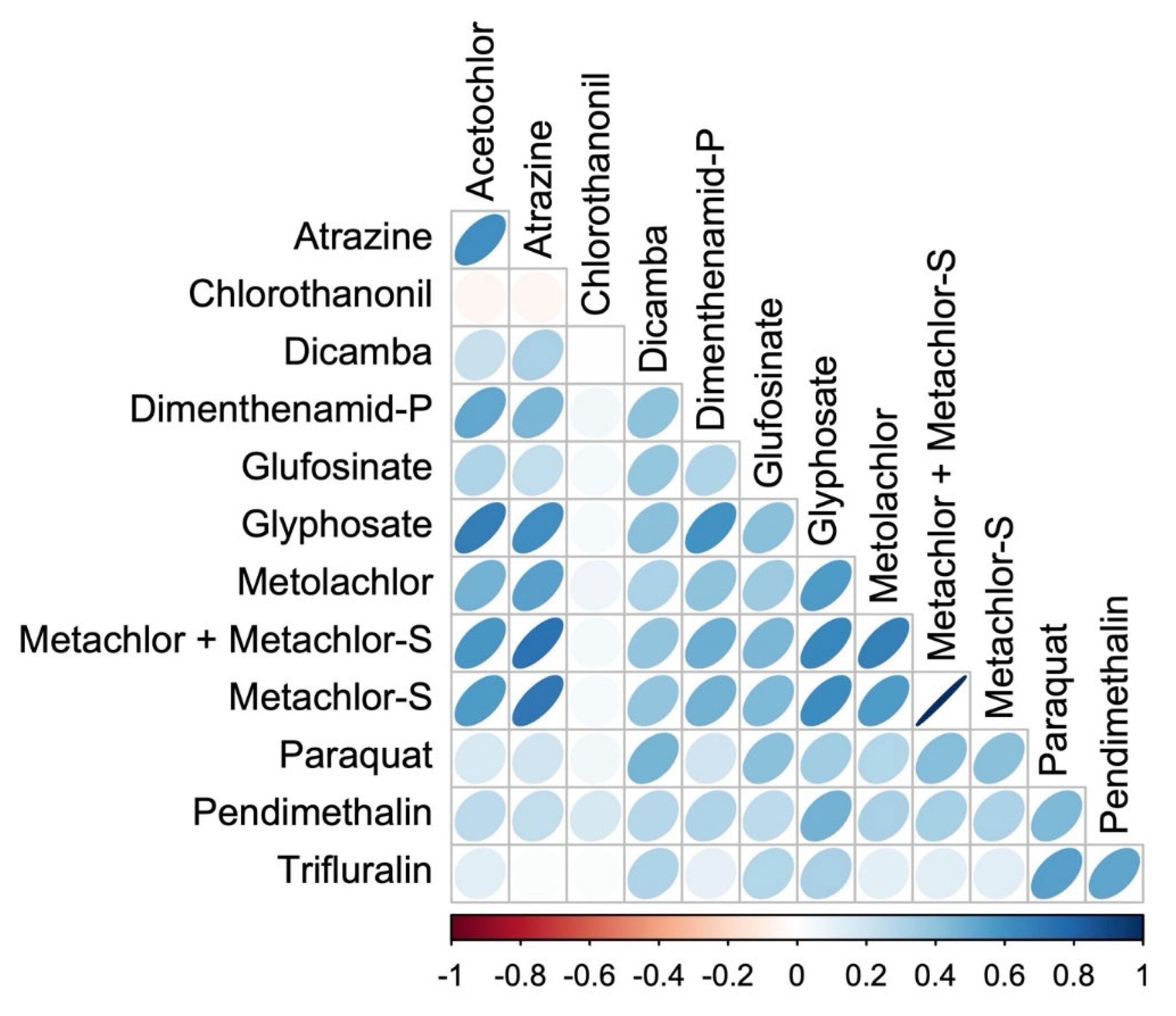
Figure B2.
Coefficient (Beta) estimates extracted from the final unreduced, adjusted, bootstrapped quantile g-computation mixture models (multi-pollutant) for associations between county level obesity rates and a mixture of herbicides from adjusted standardized models. Models are adjusted for percent smoking, percent uninsured, percent unemployed, education level, race, age (percent under 18 or over 64), study year, and NCHS rurality designation. County is included as a grouping ID. .
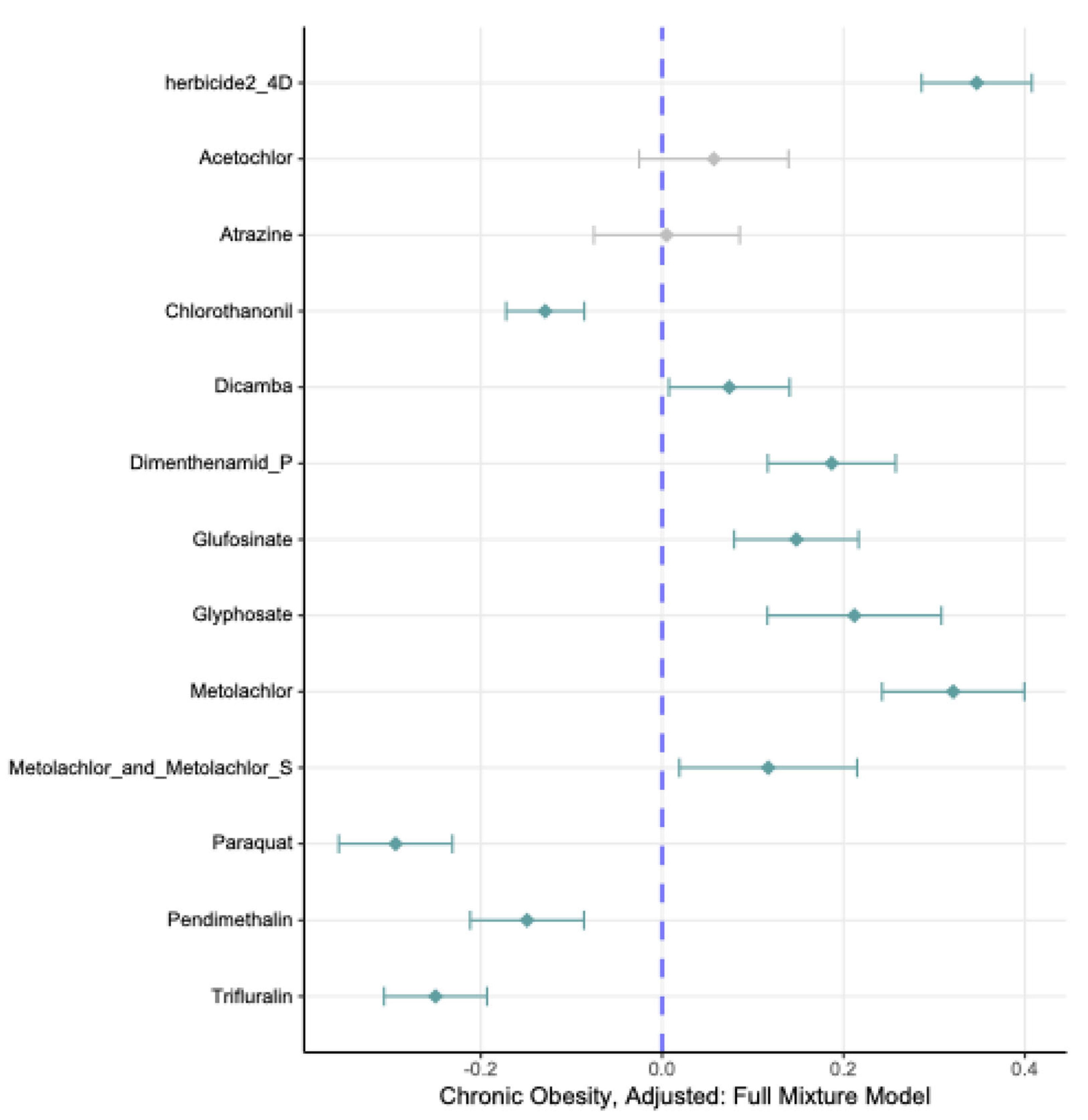
Figure B3.
EIM strengths of pairwise quantitative (direct) interactions for mixture components and Obesity rates from interaction forests including all environmental exposures and covariates. There are no qualitive (cross-over) interactions.
Figure B3.
EIM strengths of pairwise quantitative (direct) interactions for mixture components and Obesity rates from interaction forests including all environmental exposures and covariates. There are no qualitive (cross-over) interactions.
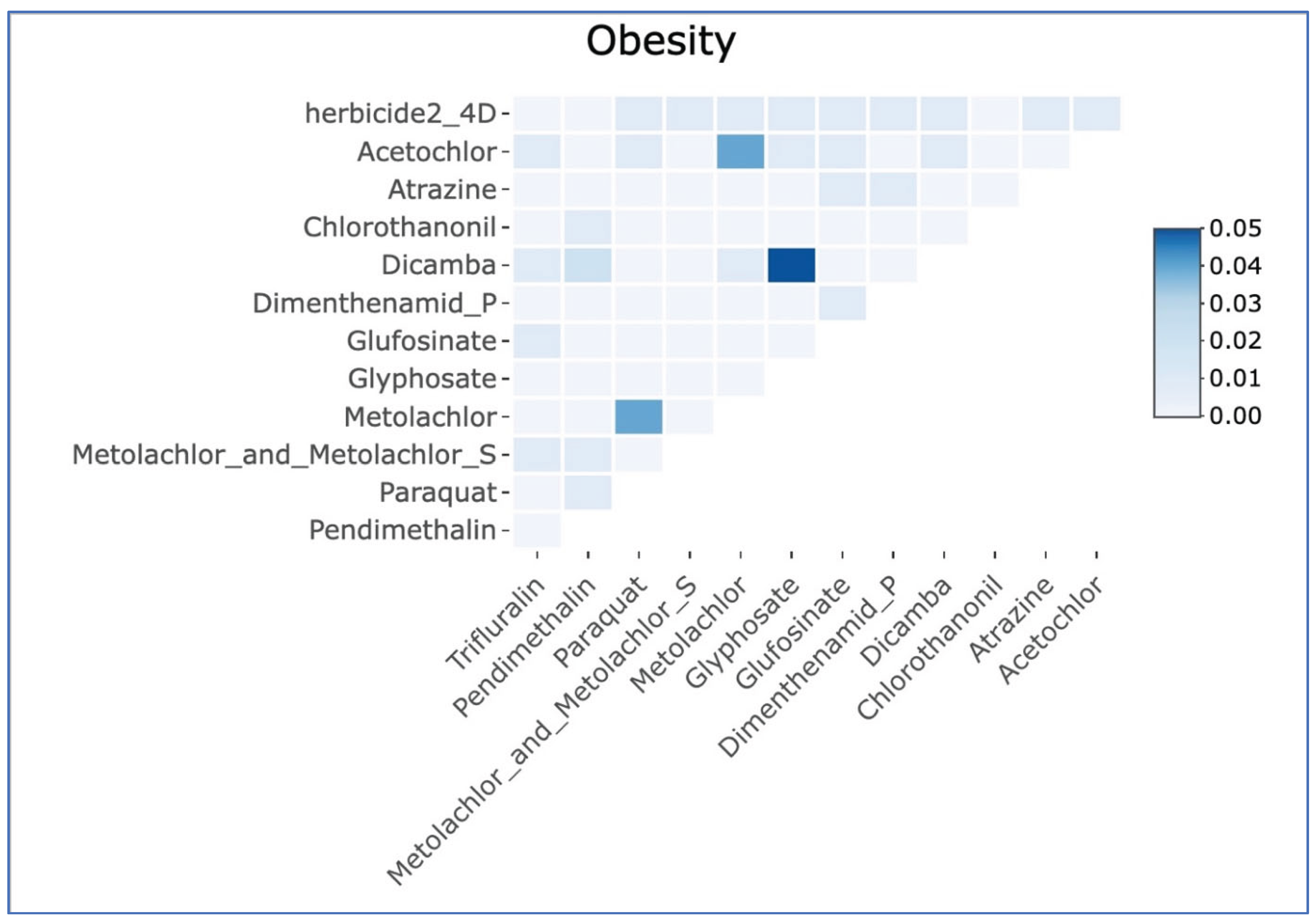

Table B2.
Herbicides applied, kilograms per (hectare)1 by county.
| Herbicide | Min | Q25 | Median | Q75 | Max |
| trifluralin | 0 | 47.5 | 290.2 | 1063.1 | 118984.0 |
| pendimethalin | 0 | 152.1 | 705.6 | 1940.6 | 127641.6 |
| paraquat | 0 | 95.7 | 424.9 | 1418.0 | 87700.0 |
| metolachlor-S | 0 | 264.1 | 2049.6 | 11095.6 | 193956.5 |
| metolachlor + metolachlor-S | 0 | 365.8 | 2727.5 | 13709.0 | 202600.2 |
| metolachlor | 0 | 86.4 | 608.8 | 2280.8 | 70608.4 |
| herbicide 2-4D | 0 | 802.9 | 2884.3 | 8000.0 | 199793.4 |
| glyphosate | 0.1 | 2015.7 | 15359.3 | 65956.5 | 594336.0 |
| glufosinate | 0 | 29.8 | 277.9 | 1456.4 | 87516.1 |
| dimenthenamid-P | 0 | 47.8 | 429.2 | 1807.8 | 49778.35 |
| dicamba | 0 | 91.4 | 369.1 | 1318.4 | 112221.9 |
| chlorothanonil | 0 | 21.8 | 127.5 | 661.7 | 176201.4 |
| atrazine | 0 | 312.4 | 2300.6 | 15193.0 | 743835.8 |
| acetochlor | 0 | 139.2 | 1335.5 | 9354.0 | 153269.7 |
1Exposures by year from Epest county level estimates 2013-2018. Pooled over 10 imputed datasets.
Table B3.
Mixture effects of spatially distributed herbicides on Obesity rates by county from crude and adjusted quantile g-computation mixture models, stratified by NCHS Urban-Rural designation. Crude models are mixture and FIPS only (included as fixed effect in crude and adjusted models). Estimated Psi () values represent increase in obesity per quantile increase in mixture exposure.
| NCHS Designation | Model | Coefficient | Estimate | 95% CI | p-value |
| Large Central Metro | Crude | intercept | 25.4 | 24.4, 26.5 | <0.0001 |
| Psi () | 0.57 | -0.14, 1.3 | 0.11 | ||
| Adjusted | intercept | 25.8 | 24.4, 27.3 | <0.0001 | |
| Psi () | 0.77 | 0.42, 1.12 | <0.0001 | ||
| Large Fringe Metro | Crude | intercept | 27.8 | 27.4, 28.2 | <0.0001 |
| Psi () | 1.23 | 0.96, 1.50 | <0.0001 | ||
| Adjusted | intercept | 27.8 | 27.2, 28.4 | <0.0001 | |
| Psi () | 0.59 | 0.4, 0.77 | <0.0001 | ||
| Medium Metro | Crude | intercept | 29.5 | 29.1, 29.9 | <0.0001 |
| Psi () | 0.71 | 0.47, 0.95 | <0.0001 | ||
| Adjusted | intercept | 28.8 | 28.3, 29.4 | <0.0001 | |
| Psi () | 0.73 | 0.55, 0.9 | <0.0001 | ||
| Small Metro | Crude | intercept | 29.5 | 29.1, 29.9 | <0.0001 |
| Psi () | 0.92 | 0.67, 1.2 | <0.0001 | ||
| Adjusted | intercept | 29.5 | 28.9, 30.1 | <0.0001 | |
| Psi () | 0.70 | 0.50, 0.90 | <0.0001 | ||
| Micropolitan | Crude | intercept | 29.4 | 29.1, 29.7 | <0.0001 |
| Psi () | 1.38 | 1.2, 1.6 | <0.0001 | ||
| Adjusted | intercept | 30.0 | 29.5, 30.4 | <0.0001 | |
| Psi () | 0.88 | 0.72, 1.04 | <0.0001 | ||
| Noncore | Crude | intercept | 30.6 | 30.35, 30.8 | <0.0001 |
| Psi () | 0.65 | 0.5, 0.8 | <0.0001 | ||
| Adjusted | intercept | 30.4 | 30.1, 30.7 | <0.0001 | |
| Psi () | 0.47 | 0.35, 0.59 | <0.0001 |
Table 4.
Rurality, obesity rates and annual herbicide application per hectare for top 14 herbicides by NCHS Urban-Rural designation (2013 standard). Highest applications across rural-urban sectors are shown in boldface dark red, and second highest in lighter red.
Table 4.
Rurality, obesity rates and annual herbicide application per hectare for top 14 herbicides by NCHS Urban-Rural designation (2013 standard). Highest applications across rural-urban sectors are shown in boldface dark red, and second highest in lighter red.
| Feature | 1NCHS Urban-Rural Designation | |||||
| Large Central Metro | Large Fringe Metro | Medium Metro | Small Metro | Micropolitan | Noncore | |
| Rurality (%) | 2.4 | 40.3 | 40.5 | 46.5 | 52.3 | 79.1 |
| Obesity rate (%) | 26.2 | 29.5 | 30.5 | 30.8 | 31.3 | 31.5 |
| Median Herbicide Application (kg/hectare) | ||||||
| acetochlor | 143 | 580 | 440 | 1290 | 1374 | 959 |
| atrazine | 321 | 1617 | 1241 | 2611 | 2734 | 1858 |
| chlorothanonil | 170 | 168 | 184 | 172 | 134 | 95 |
| dicamba | 53 | 201 | 267 | 411 | 428 | 444 |
| dimenthenamid-P | 61 | 134 | 113 | 293 | 356 | 309 |
| glufosinate | 36 | 154 | 135 | 286 | 301 | 220 |
| glyphosate | 2686 | 8449 | 7538 | 20220 | 18851 | 16838 |
| herbicide 2-4D | 656 | 1858 | 2338 | 3073 | 3404 | 3316 |
| metolachlor | 73 | 351 | 336 | 552 | 662 | 480 |
| metolachlor+metolachlor-S | 494 | 1808 | 1554 | 2800 | 3590 | 2411 |
| metolachlor-S | 421 | 1352 | 1139 | 2251 | 2581 | 1769 |
| paraquat | 91 | 310 | 376 | 509 | 456 | 412 |
| pendimethalin | 136 | 441 | 587 | 902 | 856 | 728 |
| trifluralin | 53 | 102 | 96 | 221 | 277 | 292 |
References
- Ng, M.; Fleming, T.; Robinson, M.; Thomson, B.; Graetz, N.; Margono, C.; Mullany, E.C.; Biryukov, S.; Abbafati, C.; Abera, S.F.; et al. Global, regional, and national prevalence of overweight and obesity in children and adults during 1980-2013: a systematic analysis for the Global Burden of Disease Study 2013. Lancet 2014, 384, 766–781. [Google Scholar] [CrossRef]
- Cho, N.H.; Shaw, J.E.; Karuranga, S.; Huang, Y.; da Rocha Fernandes, J.D.; Ohlrogge, A.W.; Malanda, B. IDF Diabetes Atlas: Global estimates of diabetes prevalence for 2017 and projections for 2045. Diabetes Res Clin Pract 2018, 138, 271–281. [Google Scholar] [CrossRef]
- Stackpoole, S.M.; Shoda, M.E.; Medalie, L.; Stone, W.W. Pesticides in US Rivers: Regional differences in use, occurrence, and environmental toxicity, 2013 to 2017. Sci Total Environ 2021, 787, 147147. [Google Scholar] [CrossRef] [PubMed]
- Medalie, L.; Baker, N.T.; Shoda, M.E.; Stone, W.W.; Meyer, M.T.; Stets, E.G.; Wilson, M. Influence of land use and region on glyphosate and aminomethylphosphonic acid in streams in the USA. Sci Total Environ 2020, 707, 136008. [Google Scholar] [CrossRef] [PubMed]
- Otaru, S.; Jones, L.E.; Carpenter, D.O. Associations between urine glyphosate levels and metabolic health risks: insights from a large cross-sectional population-based study. Environ Health 2024, 23, 58. [Google Scholar] [CrossRef]
- Hongoeb, J.; Tantimongcolwat, T.; Ayimbila, F.; Ruankham, W.; Phopin, K. Herbicide-related health risks: key mechanisms and a guide to mitigation strategies. J Occup Med Toxicol 2025, 20, 6. [Google Scholar] [CrossRef]
- Jayasumana, C.; Gunatilake, S.; Siribaddana, S. Simultaneous exposure to multiple heavy metals and glyphosate may contribute to Sri Lankan agricultural nephropathy. BMC Nephrol 2015, 16, 103. [Google Scholar] [CrossRef] [PubMed]
- Mesnage, R.; Defarge, N.; Spiroux de Vendômois, J.; Séralini, G.E. Potential toxic effects of glyphosate and its commercial formulations below regulatory limits. Food and chemical toxicology : an international journal published for the British Industrial Biological Research Association 2015, 84, 133–153. [Google Scholar] [CrossRef]
- Hayes, T.B.; Khoury, V.; Narayan, A.; Nazir, M.; Park, A.; Brown, T.; Adame, L.; Chan, E.; Buchholz, D.; Stueve, T.; et al. Atrazine induces complete feminization and chemical castration in male African clawed frogs (Xenopus laevis). Proc Natl Acad Sci U S A 2010, 107, 4612–4617. [Google Scholar] [CrossRef]
- Myers, J.P.; Antoniou, M.N.; Blumberg, B.; Carroll, L.; Colborn, T.; Everett, L.G.; Hansen, M.; Landrigan, P.J.; Lanphear, B.P.; Mesnage, R.; et al. Concerns over use of glyphosate-based herbicides and risks associated with exposures: a consensus statement. Environmental health : a global access science source 2016, 15. [Google Scholar] [CrossRef]
- Winchester, P.D.; Huskins, J.; Ying, J. Agrichemicals in surface water and birth defects in the United States. Acta Paediatr 2009, 98, 664–669. [Google Scholar] [CrossRef]
- Suppa, A.; Kvist, J.; Li, X.; Dhandapani, V.; Almulla, H.; Tian, A.Y.; Kissane, S.; Zhou, J.; Perotti, A.; Mangelson, H.; et al. Roundup causes embryonic development failure and alters metabolic pathways and gut microbiota functionality in non-target species. Microbiome 2020, 8. [Google Scholar] [CrossRef]
- Walsh, L.; Hill, C.; Ross, R.P. Impact of glyphosate (Roundup) on the composition and functionality of the gut microbiome. Gut Microbes 2023, 15, 2263935. [Google Scholar] [CrossRef]
- Jayaraman, S.; Krishnamoorthy, K.; Prasad, M.; Veeraraghavan, V.P.; Krishnamoorthy, R.; Alshuniaber, M.A.; Gatasheh, M.K.; Elrobh, M.; Gunassekaran. Glyphosate potentiates insulin resistance in skeletal muscle through the modulation of IRS-1/PI3K/Akt mediated mechanisms: An in vivo and in silico analysis. Int J Biol Macromol 2023, 242, 124917. [Google Scholar] [CrossRef]
- Prasad, M.; Gatasheh, M.K.; Alshuniaber, M.A.; Krishnamoorthy, R.; Rajagopal, P.; Krishnamoorthy, K.; Periyasamy, V.; Veeraraghavan, V.P.; Jayaraman, S. Impact of Glyphosate on the Development of Insulin Resistance in Experimental Diabetic Rats: Role of NFκB Signalling Pathways. Antioxidants (Basel) 2022, 11. [Google Scholar] [CrossRef]
- Ferris Pasquini, V.; Hurtazo, H.; Quintanilla, F.; Cruz-Soto, M. 2,4-Dichlorophenol Shows Estrogenic Endocrine Disruptor Activity by Altering Male Rat Sexual Behavior. Toxics 2023, 11. [Google Scholar] [CrossRef] [PubMed]
- See, W.Z.C.; Naidu, R.; Tang, K.S. Cellular and Molecular Events Leading to Paraquat-Induced Apoptosis: Mechanistic Insights into Parkinson's Disease Pathophysiology. Mol Neurobiol 2022, 59, 3353–3369. [Google Scholar] [CrossRef]
- McCormack, A.L.; Atienza, J.G.; Johnston, L.C.; Andersen, J.K.; Vu, S.; Di Monte, D.A. Role of oxidative stress in paraquat-induced dopaminergic cell degeneration. J Neurochem 2005, 93, 1030–1037. [Google Scholar] [CrossRef] [PubMed]
- Dinić, S.; Arambašić Jovanović, J.; Uskoković, A.; Mihailović, M.; Grdović, N.; Tolić, A.; Rajić, J.; Đorđević, M.; Vidaković, M. Oxidative stress-mediated beta cell death and dysfunction as a target for diabetes management. Front Endocrinol (Lausanne) 2022, 13, 1006376. [Google Scholar] [CrossRef]
- Yesupatham, A.; Saraswathy, R. Role of oxidative stress in prediabetes development. Biochem Biophys Rep 2025, 43, 102069. [Google Scholar] [CrossRef] [PubMed]
- Carpenter, D.O.; Arcaro, K.; Spink, D.C. Understanding the human health effects of chemical mixtures. Environ Health Perspect 2002, 110, 25–42. [Google Scholar] [CrossRef] [PubMed]
- Heys, K.A.; Shore, R.F.; Pereira, M.G.; Jones, K.C.; Martin, F.L. Risk assessment of environmental mixture effects. RSC Advances 2016, 6, 47844–47857. [Google Scholar] [CrossRef]
- Lagunas-Rangel, F.A.; Linnea-Niemi, J.V.; Kudłak, B.; Williams, M.J.; Jönsson, J.; Schiöth, H.B. Role of the Synergistic Interactions of Environmental Pollutants in the Development of Cancer. Geohealth 2022, 6, e2021GH000552. [Google Scholar] [CrossRef] [PubMed]
- Wagner, V.; Antunes, P.M.; Irvine, M.; Nelson, C.R. Herbicide usage for invasive non-native plant management in wildland areas of North America. J Appl Ecol 2017, 54, 198–204. [Google Scholar] [CrossRef]
- Rojas, J.; Dhar, A.; Naeth, M. Urban naturalization for green spaces using soil tillage, herbicide application, compost amendment and native vegetation. Land 2021, 10. [Google Scholar] [CrossRef]
- Curl, C.L.; Hyland, C.; Spivak, M.; Sheppard, L.; Lanphear, B.; Antoniou, M.N.; Ospina, M.; Calafat, A.M. The Effect of Pesticide Spray Season and Residential Proximity to Agriculture on Glyphosate Exposure among Pregnant People in Southern Idaho, 2021. Environ Health Perspect 2023, 131, 127001. [Google Scholar] [CrossRef]
- De Troeyer, K.; Casas, L.; Bijnens, E.M.; Bruckers, L.; Covaci, A.; De Henauw, S.; Den Hond, E.; Loots, I.; Nelen, V.; Verheyen, V.J.; et al. Higher proportion of agricultural land use around the residence is associated with higher urinary concentrations of AMPA, a glyphosate metabolite. Int J Hyg Environ Health 2022, 246, 114039. [Google Scholar] [CrossRef] [PubMed]
- Hyland, C.; Spivak, M.; Sheppard, L.; Lanphear, B.P.; Antoniou, M.; Ospina, M.; Calafat, A.M.; Curl, C.L. Urinary Glyphosate Concentrations among Pregnant Participants in a Randomized, Crossover Trial of Organic and Conventional Diets. Environ Health Perspect 2023, 131, 77005. [Google Scholar] [CrossRef]
- USGS. Pesticide National Synthesis Project. Available online: https://water.usgs.
- Remington, P.L.; Catlin, B.B.; Gennuso, K.P. The County Health Rankings: rationale and methods. Popul Health Metr 2015, 13, 11. [Google Scholar] [CrossRef]
- Hood, C.M.; Gennuso, K.P.; Swain, G.R.; Catlin, B.B. County Health Rankings: Relationships Between Determinant Factors and Health Outcomes. Am J Prev Med 2016, 50, 129–135. [Google Scholar] [CrossRef]
- Carlson, S.A.; Watson, K.B.; Rockhill, S.; Wang, Y.; Pankowska, M.M.; Greenlund, K.J. Linking Local-Level Chronic Disease and Social Vulnerability Measures to Inform Planning Efforts: A COPD Example. Prev Chronic Dis 2023, 20, E76. [Google Scholar] [CrossRef]
- Vo, A.; Tao, Y.; Li, Y.; Albarrak, A. The Association Between Social Determinants of Health and Population Health Outcomes: Ecological Analysis. JMIR Public Health Surveill 2023, 9, e44070. [Google Scholar] [CrossRef]
- Ibrahim, R.; Habib, A.; Terrani, K.; Ravi, S.; Takamatsu, C.; Salih, M.; Ferreira, J.P. County-level variation in healthcare coverage and ischemic heart disease mortality. PLoS One 2024, 19, e0292167. [Google Scholar] [CrossRef] [PubMed]
- Zhang, X.; Holt, J.B.; Lu, H.; Wheaton, A.G.; Ford, E.S.; Greenlund, K.J.; Croft, J.B. Multilevel regression and poststratification for small-area estimation of population health outcomes: a case study of chronic obstructive pulmonary disease prevalence using the behavioral risk factor surveillance system. Am J Epidemiol 2014, 179, 1025–1033. [Google Scholar] [CrossRef] [PubMed]
- Zhang, X.; Holt, J.B.; Yun, S.; Lu, H.; Greenlund, K.J.; Croft, J.B. Validation of multilevel regression and poststratification methodology for small area estimation of health indicators from the behavioral risk factor surveillance system. Am J Epidemiol 2015, 182, 127–137. [Google Scholar] [CrossRef]
- McCullough, M.L.; Chantaprasopsuk, S.; Islami, F.; Rees-Punia, E.; Um, C.Y.; Wang, Y.; Leach, C.R.; Sullivan, K.R.; Patel, A.V. Association of Socioeconomic and Geographic Factors With Diet Quality in US Adults. JAMA Netw Open 2022, 5, e2216406. [Google Scholar] [CrossRef] [PubMed]
- Rubin, D.B. Multiple Imputation for Nonresponse in Surveys; Wiley-Interscience: 1987, 2004; p. 258. [Google Scholar]
- Rubin, D.B. Multiple Imputation for Nonresponse in Surveys; Wiley: 2009.
- Benjamini, Y.; Hochberg, Y. Controlling the False Discovery Rate: A Practical and Powerful Approach to Multiple Testing. Journal of the Royal Statistical Society: Series B (Methodological) 1995, 57, 289–300. [Google Scholar] [CrossRef]
- Bobb, J.F.; Valeri, L.; Claus Henn, B.; Christiani, D.C.; Wright, R.O.; Mazumdar, M.; Godleski, J.J.; Coull, B.A. Bayesian kernel machine regression for estimating the health effects of multi-pollutant mixtures. Biostatistics 2015, 16, 493–508. [Google Scholar] [CrossRef]
- Bobb, J.F.; Claus Henn, B.; Valeri, L.; Coull, B.A. Statistical software for analyzing the health effects of multiple concurrent exposures via Bayesian kernel machine regression. Environ Health 2018, 17, 67. [Google Scholar] [CrossRef]
- Keil, A.P.; Buckley, J.P.; O'Brien, K.M.; Ferguson, K.K.; Zhao, S.; White, A.J. A Quantile-Based g-Computation Approach to Addressing the Effects of Exposure Mixtures. Environ Health Perspect 2020, 128, 47004. [Google Scholar] [CrossRef]
- Hornung, R.; Boulesteix, A.-L. Interaction forests: Identifying and exploiting interpretable quantitative and qualitative interaction effects. Comput Stat Data Anal 2022, 171, 107460. [Google Scholar] [CrossRef]
- Peluso, A.; Rastogi, D.; Klasky, H.B.; Logan, J.; Maguire, D.; Grant, J.; Christian, B.; Hanson, H.A. Environmental determinants of health: Measuring multiple physical environmental exposures at the United States census tract level. Health Place 2024, 89, 103303. [Google Scholar] [CrossRef]
- Madani, N.A.; Carpenter, D.O. Patterns of Emergency Room Visits for Respiratory Diseases in New York State in Relation to Air Pollution, Poverty and Smoking. Int J Environ Res Public Health 2023, 20. [Google Scholar] [CrossRef]
- Doogan, N.J.; Roberts, M.E.; Wewers, M.E.; Stanton, C.A.; Keith, D.R.; Gaalema, D.E.; Kurti, A.N.; Redner, R.; Cepeda-Benito, A.; Bunn, J.Y.; et al. A growing geographic disparity: Rural and urban cigarette smoking trends in the United States. Prev Med 2017, 104, 79–85. [Google Scholar] [CrossRef]
- Parker, M.A.; Weinberger, A.H.; Eggers, E.M.; Parker, E.S.; Villanti, A.C. Trends in Rural and Urban Cigarette Smoking Quit Ratios in the US From 2010 to 2020. JAMA Netw Open 2022, 5, e2225326. [Google Scholar] [CrossRef] [PubMed]
- Eskenazi, B.; Gunier, R.B.; Rauch, S.; Kogut, K.; Perito, E.R.; Mendez, X.; Limbach, C.; Holland, N.; Bradman, A.; Harley, K.G.; et al. Association of Lifetime Exposure to Glyphosate and Aminomethylphosphonic Acid (AMPA) with Liver Inflammation and Metabolic Syndrome at Young Adulthood: Findings from the CHAMACOS Study. Environ Health Perspect 2023, 131, 37001. [Google Scholar] [CrossRef] [PubMed]
- Glover, F.; Jean-Baptiste, O.; Del Giudice, F.; Belladelli, F.; Seranio, N.; Muncey, W.; Eisenberg, M. The association between glyphosate exposure and metabolic syndrome among US adults. Human and Ecological Risk Assessment: An International Journal. 2023, 29, 1212–1225. [Google Scholar] [CrossRef]
Figure 1.
Forest plot of single-pollutant results for associations between county level obesity rates and herbicide applications from adjusted mixed effects models, years 2013 to 2018. Results pooled over 10 imputed datasets.
Figure 1.
Forest plot of single-pollutant results for associations between county level obesity rates and herbicide applications from adjusted mixed effects models, years 2013 to 2018. Results pooled over 10 imputed datasets.
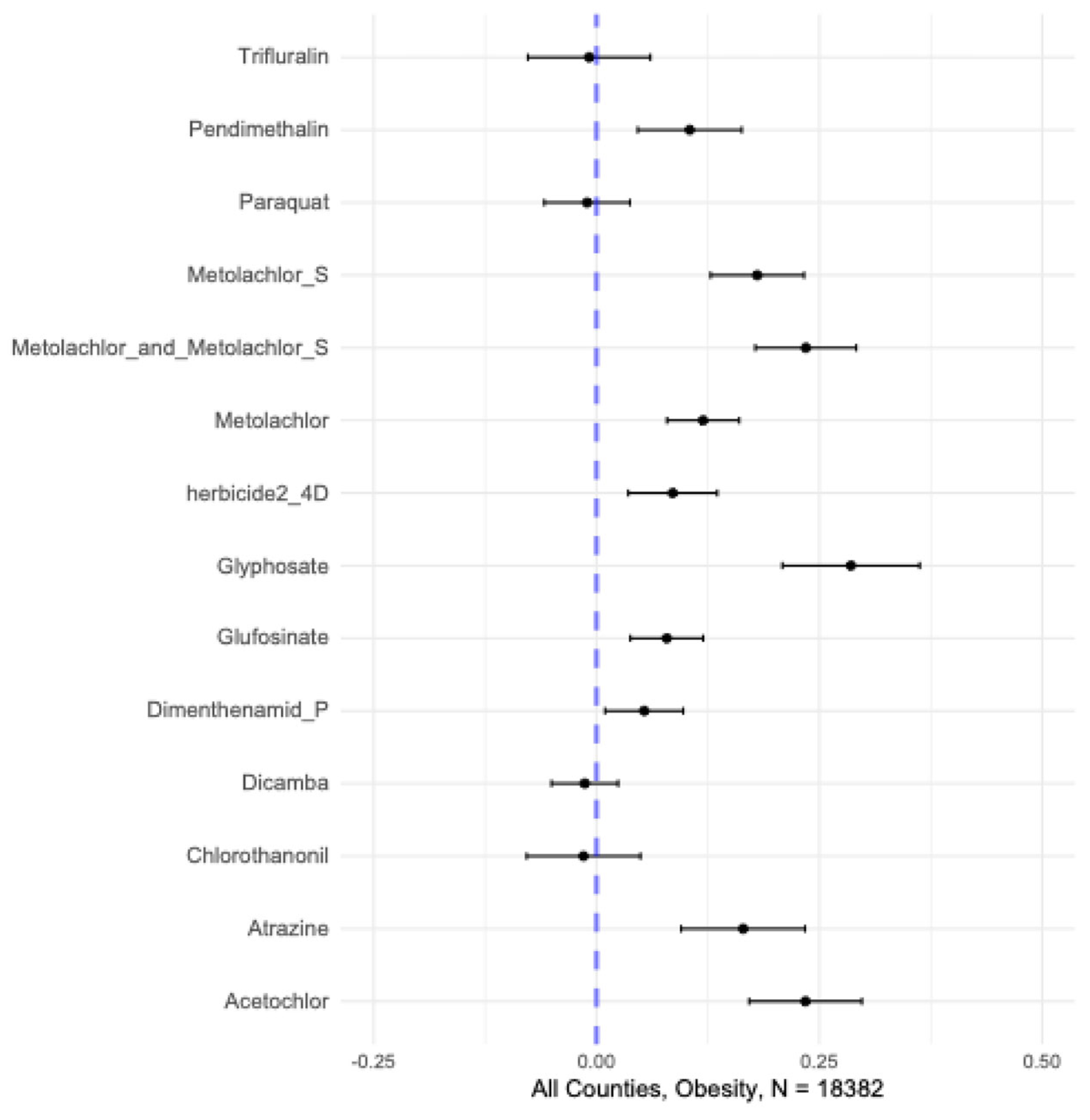
Figure 2.
Mixture weightings from the final adjusted (unreduced) quantile g-computation mixture models for county level obesity rates. Negative weights are shown in pale blue and positive weights in dark blue. Results are pooled over 10 imputed datasets. Metolachlor-S is omitted from the mixture models due to very high correlation with other Metolachlor species (See Figure S1). For a coefficient (Beta estimate) forest plot from the final fitted mixture model, please see supplemental Figure S2.
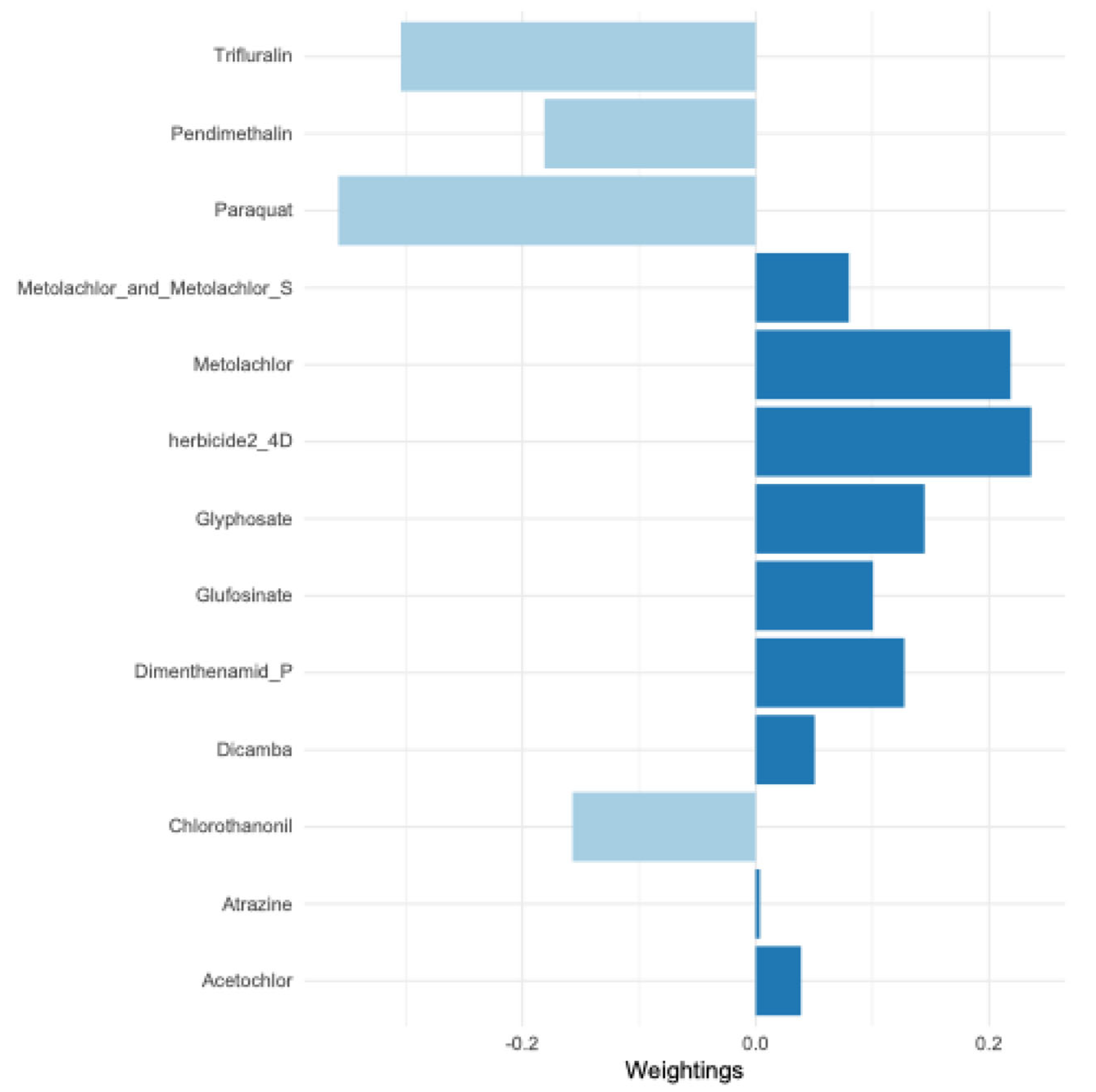
Figure 3.
Forest plot of mixture effects (Psi) from subgroups analysis via mixture models stratified on NCHS urban-rural designation, presented with confidence intervals. Adjusted models are shown in dark rose, and mixture only (crude) models are shown in pale blue.
Figure 3.
Forest plot of mixture effects (Psi) from subgroups analysis via mixture models stratified on NCHS urban-rural designation, presented with confidence intervals. Adjusted models are shown in dark rose, and mixture only (crude) models are shown in pale blue.
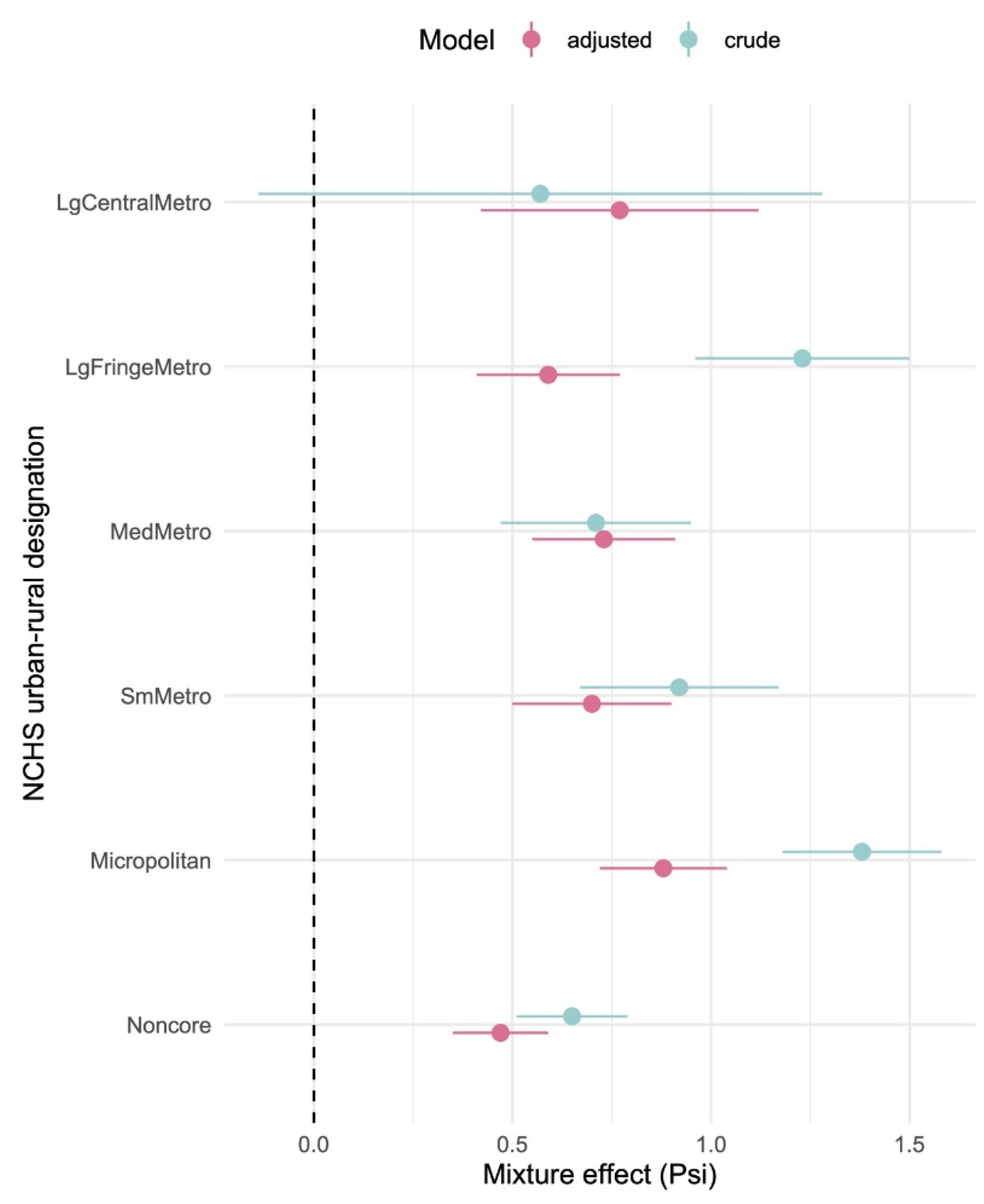
Figure 4.
Median herbicide application by NCHS urban-rural designation (kg/hectare/year). See also Appendix Table B4.
Figure 4.
Median herbicide application by NCHS urban-rural designation (kg/hectare/year). See also Appendix Table B4.
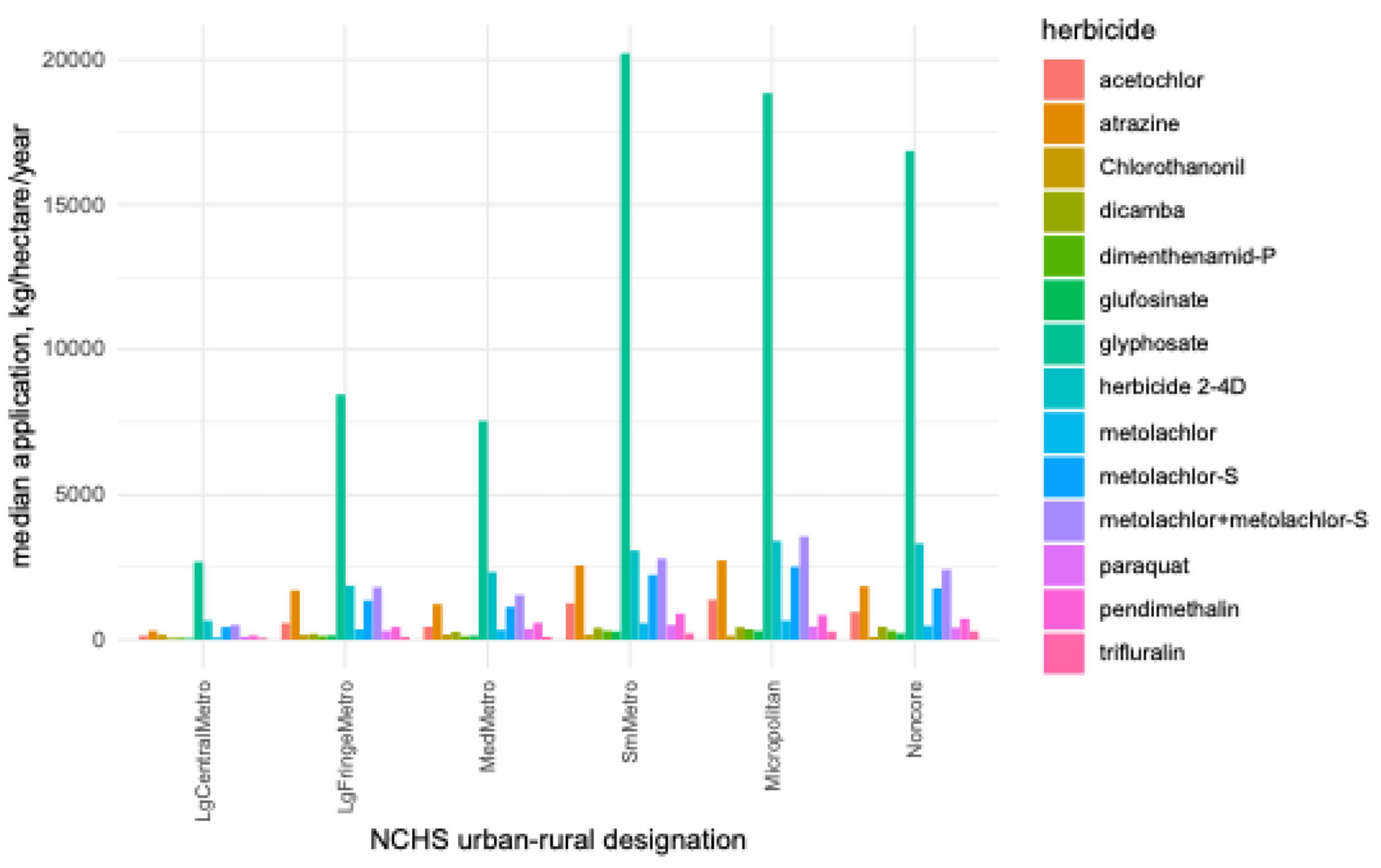
Table 1.
Population/demographic variables (N=18,382), Years 2013-2018. Summarized from imputed data.
Table 1.
Population/demographic variables (N=18,382), Years 2013-2018. Summarized from imputed data.
| Covariate (%) | Mean | Median | IQR | |
| Outcome | Obese | 30.9 | 31.0 | [29.0, 34.0] |
| Risk factors | Smoking | 19.4 | 19.0 | [16.0, 22.0] |
| Uninsured | 17.0 | 16.9 | [12.0, 21.0] | |
| Unemployed | 6.7 | 6.3 | [4.7, 8.1] | |
| Rurality | 60.3 | 60.7 | [35.2, 88.9] | |
| Food Insecure | 13.6 | 14.0 | [11.0, 16.0] | |
| education | High School Graduate | 84.1 | 86.0 | [79.0, 91.0] |
| Some College | 55.8 | 55.8 | [47.6, 64.3] | |
| Age | Population < 18 years | 22.7 | 22.6 | [20.7, 24.4] |
| Population > 64 years | 17.4 | 17.1 | [11.5, 13.8] | |
|
Race (percent) |
Non-Hispanic White | 77.9 | 86.3 | [68.2, 93.9] |
| Black/African American | 8.8 | 2.0 | [0.6, 9.3] | |
| Asian | 1.3 | 0.6 | [0.4, 1.1] | |
| Hispanic | 8.9 | 3.5 | [1.9, 8.0] | |
| Native American | 1.9 | 0.6 | [0.3, 1.1] | |
| Pacific Islander | 0.08 | 0.0 | [0.0, 0.10] | |
| Level | Number counties | (Percent) | ||
|
1NCHS Urban-Rural Designation |
Large Central Metro | 351 | (1.9%) | |
| Large Fringe Metro | 2130 | (11.6) | ||
| Medium Metropolitan | 2190 | (11.9) | ||
| Small Metro | 2094 | (11.4) | ||
| Micropolitan | 3803 | (20.7) | ||
| Noncore | 7814 | (42.5) | ||
Table 2.
Estimates (per standard deviation exposure) from adjusted single-pollutant mixed effects models for associations between herbicide application rates per hectare and county level obesity rates. Results are shown as forest plot visualizations in Figure 1.
Table 2.
Estimates (per standard deviation exposure) from adjusted single-pollutant mixed effects models for associations between herbicide application rates per hectare and county level obesity rates. Results are shown as forest plot visualizations in Figure 1.
| Herbicide | Estimate | 95% Confidence Interval | p-value |
FDR adjusted |
| acetochlor | 0.23 | 0.17, 0.30 | <0.0001 | <0.0001 |
| atrazine | 0.16 | 0.095, 0.23 | <0.0001 | <0.0001 |
| glufosinate | 0.08 | 0.038, 0.12 | <0.0001 | <0.0001 |
| glyphosate | 0.29 | 0.21, 0.36 | <0.0001 | <0.0001 |
| metolachlor | 0.12 | 0.08, 0.16 | <0.0001 | <0.0001 |
| metolachlor + metolachlor-S | 0.24 | 0.18, 0.29 | <0.0001 | <0.0001 |
| metolachlor-S | 0.18 | 0.13, 0.23 | <0.0001 | <0.0001 |
| pendimethalin | 0.11 | 0.046, 0.16 | <0.0001 | <0.0001 |
| herbicide 2-4D | 0.09 | 0.036, 0.135 | 0.001 | 0.002 |
| dimenthenamid-P | 0.05 | 0.01, 0.097 | 0.02 | 0.04 |
| dicamba | -0.013 | -0.05, 0.024 | 0.49 | 0.62 |
| chlorothanonil | -0.02 | -0.078, 0.049 | 0.66 | 0.72 |
| paraquat | -0.01 | -0.0, 0.038 | 0.67 | 0.72 |
| trifluralin | -0.008 | -0.077, 0.06 | 0.81 | 0.81 |
Table 3.
Mixture effects of county level herbicide applications on Obesity rates from crude and adjusted quantile g-computation mixture models (Keil et al. 2020). Results for crude (mixture and FIPS code only) and adjusted models, including interactants with nonzero EIM identified via interaction forest runs, i.e., glyphosate x dicamba, metolachlor x paraquat, and metolachlor x acetochlor, are shown below the solid line. Estimated Psi () values represent increase in county level obesity rates per quantile increase in county level exposure mixture.
| Model | Coefficient | Estimate | 95% Confidence Interval | p-value |
| Crude | intercept | 29.5 | 29.4, 29.6 | <0.0001 |
| Psi () | 1.0 | 0.94, 1.1 | <0.0001 | |
| Adjusted | intercept | 28.0 | 27.6, 28.4 | <0.0001 |
| Psi () | 0.71 | 0.65, 0.76 | <0.0001 | |
| Crude + interactants |
intercept | 29.4 | 29.3, 29.6 | <0.0001 |
| Psi () | 1.4 | 1.2, 1.6 | <0.0001 | |
| Adjusted + interactants |
intercept | 28.1 | 27.7, 28.5 | <0.0001 |
| Psi () | 0.68 | 0.50, 0.86 | <0.0001 |
Disclaimer/Publisher’s Note: The statements, opinions and data contained in all publications are solely those of the individual author(s) and contributor(s) and not of MDPI and/or the editor(s). MDPI and/or the editor(s) disclaim responsibility for any injury to people or property resulting from any ideas, methods, instructions or products referred to in the content. |
© 2025 by the authors. Licensee MDPI, Basel, Switzerland. This article is an open access article distributed under the terms and conditions of the Creative Commons Attribution (CC BY) license (http://creativecommons.org/licenses/by/4.0/).
Copyright: This open access article is published under a Creative Commons CC BY 4.0 license, which permit the free download, distribution, and reuse, provided that the author and preprint are cited in any reuse.


