Submitted:
15 August 2025
Posted:
18 August 2025
You are already at the latest version
Abstract
Achieving carbon neutrality, enhancing energy efficiency, planning renewable energy installations, ensuring energy supply security, and accurately addressing energy demand are among the most critical global energy priorities. In this context, energy demand forecasting plays a pivotal role in shaping energy policies and ensuring systematic planning. Accurate demand-side forecasting contributes to improved energy efficiency and the formulation of long-term strategic energy policies. This study focuses on forecasting Turkey’s geothermal, wind, and solar energy consumption for the period 2025–2030 using five years of historical consumption data. A total of eight different regression-based forecasting models were employed. By validating model accuracy with 2023–2024 data, a hybrid prediction model was developed to generate reliable forecasts for 2025–2030. In the hybrid estimation model, the impact power of the variables affecting the formation of demand was calculated using the Pearson Correlation Statistical method. The results aim to support data-driven energy planning and policy development in alignment with sustainability goals.
Keywords:
Energy demand forecasting
; Hybrid forecasting model
; Energy planning in Turkey
; Energy Strategy
1. Introduction
In a globalizing world, increasing population rates, industrialization, technological advancements, and the decline of energy supply resources are pushing energy issues to the forefront of the world's agenda. Numerous studies are being conducted in countries to address this issue. These include energy demand forecasting studies and demand management, energy supply security studies, renewable energy applications, and the analysis and direction of energy policies. Energy demand forecasting is a prominent example of this type of research.
Energy demand forecasting is the estimation of energy demand over specific time frames, taking into account future data and changing parameters. Forecasting studies provide short-term, medium-term, and long-term energy consumption and production plans, providing roadmaps for countries, policymakers, and individual and corporate consumers.
The purpose of energy demand forecasting is to achieve supply-demand balance, implement infrastructure plans, create optimal sizing by considering peak and trough loads, increase energy efficiency, and develop plans for achieving carbon neutrality.
Energy demand forecasting studies are classified according to time scale and forecasting methods. Studies conducted based on time scales are categorized into three categories: short-term, medium-term, and long-term. Short-term studies utilize intraday, day-ahead, and balancing market data to generate hourly and daily forecasts. Medium-term forecasting models utilize monthly and annual forecasts. Long-term models utilize forecasts for periods of 3, 5, 10, or longer.
Energy demand forecasts are categorized into four types based on forecasting methods: statistical methods, machine learning methods, artificial neural network models, and hybrid models.
Numerous studies have been conducted in the literature using forecasting methods. Time series modeling is among the traditional methods in this field. ARIMA, SARIMA, and similar techniques, in particular, have provided effective solutions for identifying historical patterns (Dudek, 2020), (Lee & Cho, 2021),( Sharma & Verma, 2023). However, the fact that these models are based on linear assumptions and cannot adequately reflect the impact of sudden changes and external factors has led to the need for more flexible models. Some studies have shown that statistical methods can provide similar levels of accuracy in certain scenarios compared to artificial neural network models (Zhang & Zhou, 2020),( Yılmaz, 2023).
Machine learning algorithms are frequently applied in energy demand forecasting. Methods such as SVR, Random Forest, and decision trees, in particular, have demonstrated success in learning nonlinear relationships, (Li, Zhang & Chen, 2024),( Al-Qahtani, Elleithy & Alotaibi, 2021),( Sarkar, Roy & Das, 2022).There are examples in the literature where prediction accuracy has been significantly improved by optimizing support vector regression models with genetic algorithms . Furthermore, feature engineering approaches applied to variable selection have also been shown to increase model performance (Al-Qahtani, Elleithy & Alotaibi, 2021), (Kumar, Ranjan & Tiwari, 2023).
Deep learning architectures are one of the areas where the most remarkable advances in energy forecasting have been made. Network structures such as LSTM, GRU, and CNN-LSTM produce effective results on time-dependent data (Roy, Maity & Ghosh, 2021),( Doğan, Kaya & Öztürk, 2024),( Khan, Taj & Smith, 2024). Thanks to the powerful structure of LSTM in sequential data analysis, it has become possible to model the long-term effects of past data . Furthermore, it has been reported that short-term sudden changes in hybrid structures can be successfully learned by integrating LSTM and CNN (Mehmood & Iqbal, 2022).
Hybrid systems that combine different model structures offer the advantages of both statistical components and artificial intelligence models. When seasonal decomposition-based models such as Prophet are combined with deep learning techniques such as LSTM, different dynamics in time series can be analyzed separately (Akçay & Altuğ, 2024). These approaches have enabled higher accuracy rates, especially in regions where seasonal effects are pronounced or sudden demand fluctuations are frequently experienced (Arif & Hussain, 2023),( Akçay & Altuğ, 2024).
Current research trends propose more accurate modeling of energy demand not only with historical consumption data but also with multiple data sources such as climate data, economic indicators, social mobility, and electric vehicle usage statistics . Such multivariate models have made significant contributions to predicting changing consumption habits, especially in the post-pandemic period (Wang, Yu & Zhang, 2023).
Transformer models, one of the new-generation neural network structures, have recently been incorporated into the energy estimation literature. Their success in learning long-term dependencies demonstrates that they have more advanced estimation capabilities compared to classical LSTM or GRU architectures (Kim, Jang & Lee, 2024). Research conducted in the context of Turkey also reflects these global trends. Studies that have presented comparative analyses of methods such as LSTM, Prophet, ARIMA, and Random Forest applied to different regions have demonstrated that hybrid approaches provide superior performance, particularly in short-term forecasting (Demirtaş & Şahin, 2024).It is also emphasized that models adapted to local datasets can produce more effective results than universal models.
A study in (Wang & Li, 2020), analyzed China's electricity demand using the ARIMA model, demonstrating the model's short-term forecasting success. (Alwee, Yusof & Ismail, 2014) compared Exponential Smoothing methods with different parameter sets, achieving high accuracy in industrial consumption forecasts, particularly with the Holt-Winters model. (Mohamed & Kamel, 2015), compared linear regression and an MLP-based artificial neural network, demonstrating that the artificial neural network significantly reduces error rates compared to the linear model. In (Şahin & Karabacak, 2018), Türkiye's annual electricity consumption was modeled using Polynomial Regression, and it was determined that 3rd-degree polynomials gave more appropriate results. In (Zhang, Zhou & Chen, 2020), Lasso and Ridge Regression were tested together, and their performance against overfitting was measured; it was shown that Lasso provided an advantage in terms of variable selection. In (Khosravi, Ghadimi & Dehghanian, 2019), consumption data were modeled using the Random Forest method, and it was shown that the model learned seasonal effects particularly well. In (Ahmad & Chen, 2017), energy demand was estimated using SVR (Support Vector Regression), and better prediction performance was obtained with the RBF kernel compared to other kernel functions. In (Liu, Wang & Zhang, 2019), energy consumption was estimated using the XGBoost algorithm, and it was determined that the model gave lower RMSE values, especially after hyperparameter optimization, compared to other methods. In (Deb, Zhang & Lee, 2017), all machine learning-based methods (SVR, RF, XGBoost, ANN) were compared, and it was found that ensemble methods were more successful than individual models. In (Fazel Zarandi, Hosseini & Turksen, 2020), the ARIMA-XGBoost model was developed using hybrid approaches, and it was stated that both trends and seasonal fluctuations were captured more accurately.
In this study, using Turkey's current 2020-2024 consumption data, the 2025-2030 wind-solar-geothermal energy demand was estimated using ARIMA, Exponential Smoothing, Linear Regression, Artificial Neural Network (MLP), Polynomial Regression, Lasso, Random Forest, Ridge, Support Vector Regression (SVR), and Gradient Boosting (XGBoost) forecasting methods. Post-calculation backtesting was conducted, the models that produced the best results were identified, and the hybrid forecasting method was developed and implemented.
Unlike other studies, this study employed eight different forecasting methods and conducted cross-analysis. A new hybrid model was developed and applied to the same data set, and the results were compared with each forecasting method. A renewable approach is presented by using Türkiye's wind, geothermal, and solar energy consumption as a dataset.
In the study, gross domestic product, population and number of university graduates for the years 2019-2024 were taken into account as independent variables.
The study methodology consisted of data collection and processing into meaningful data, establishing and implementing forecasting models based on the data, validating the forecasts with test data, conducting model performance tests, and determining the hybrid model. In this context, a forecast based on production values was conducted in the study. Data on wind, solar, and geothermal energy consumed in Turkey between 2019 and 2024 were obtained from the Turkish Ministry of Energy and Natural Resources. The data was then processed into meaningful data. The forecast model was created using ARIMA, Exponential Smoothing, Linear Regression, Artificial Neural Network (MLP), Polynomial Regression, Lasso, Random Forest, Ridge, Support Vector Regression (SVR), and Gradient Boosting (XGBoost). The forecast was concluded with retrospective accuracy testing, determining optimal forecasting methods, and creating and implementing a hybrid forecasting system based on these data. Energy consumption data served as the dependent variables in the forecasting studies. The results were analyzed comparatively, and a wind-solar-geothermal energy consumption forecast for 2025-2030 was produced. In the hybrid estimation model, the impact power of the variables affecting the formation of demand was calculated using the Pearson Correlation Statistical method. The flow diagram of the study is shown in Figure 1.
1. Creating the Data Set
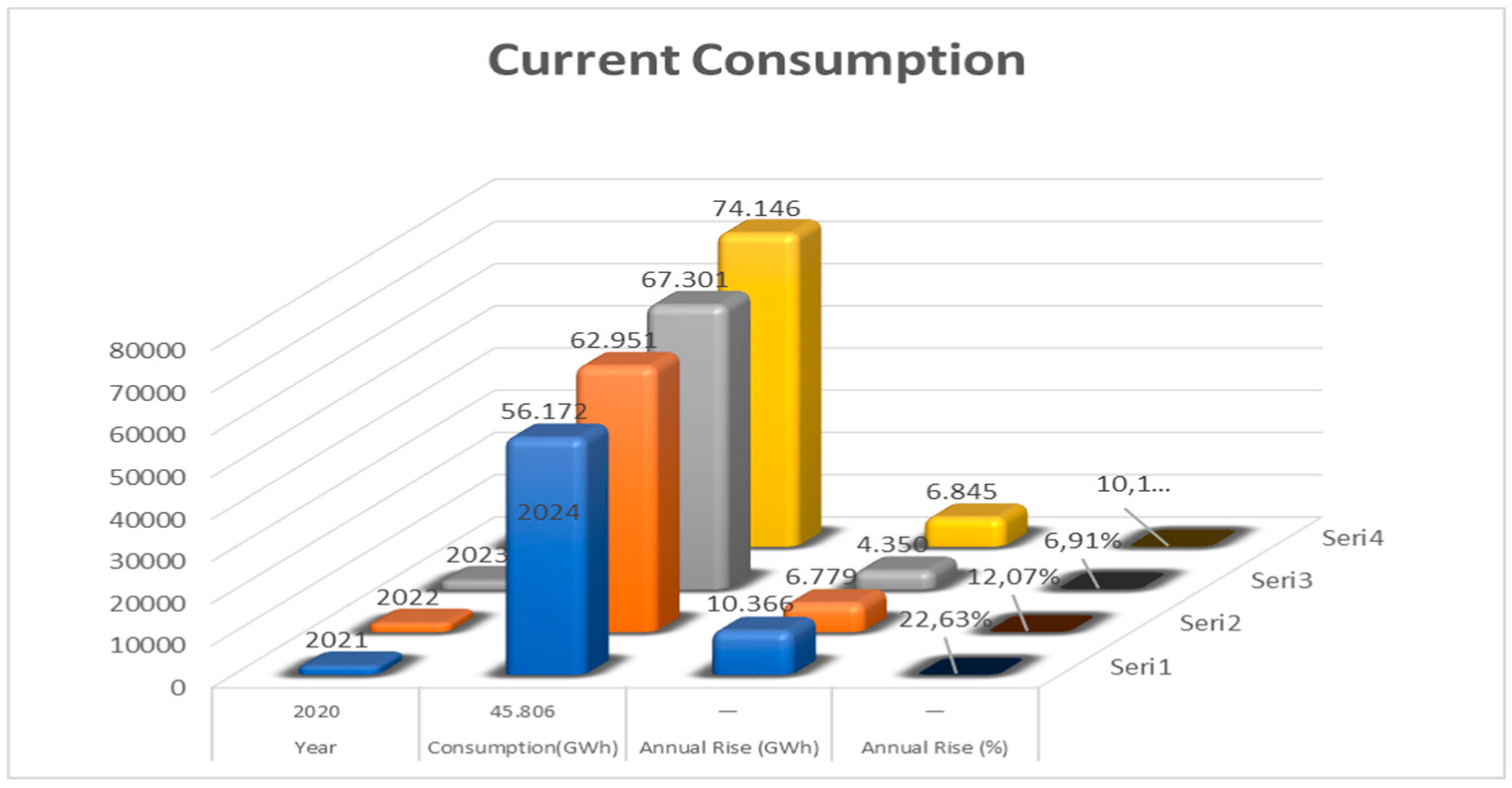
Five-year consumption data from the Turkish Ministry of Energy and Natural Resources, covering the years 2019-2024, were analyzed, compiled, and adapted for model use. Total annual consumption data for these resources was obtained based solely on wind, solar, and geothermal energy data.
Figure 2.
Real Consumption Values Of Turkey 2020-2024 Geothermal, Solar, And Wind Energy.
2. Creating and Implementing Forecast Models
The forecasting model was created using ARIMA, Linear Regression, Exponential Smoothing, Polynomial Regression, Random Forest Regressor, XGBoost Regressor, Lasso, Ridge, and SVR forecasting methods on the same dataset.
In the study conducted using ARIMA (AutoRegressive Integrated Moving Average), annual production values were obtained, and trend testing was performed using these values. After selecting the model parameters, the most appropriate p, d, and q values were determined. Forward-looking forecasting was performed using the past 5 years of data. A mathematical equation was created: p: Autoregressive term (AR), d: Differencing number (if there is a trend), q: Moving average (MA), and ϵt: White noise error term. Stationarity Test – ADF Test One of the basic assumptions of the ARIMA model is that the data is stationary. According to the ADF (Augmented Dickey-Fuller) test, the solar production data is not stationary because it contains a trend. It became stationary when the 1st degree difference was taken.
Model Parameter Selection: AR (p), MA (q). To determine these, the ACF (Autocorrelation Function) graph and the PACF (Partial Autocorrelation Function) graph were used. The ACF rapidly decreased to zero after the first delay → the MA component was low, the PACF decayed slowly → the AR component was more significant. Therefore, the most suitable model was found to be ARIMA(2,1,1) according to the AIC criterion. Parameter training was initiated. The trained parameters are shown in Table 1.
The Linear Regression Model is a model that makes future predictions using linear equations. This model performs regression using year information. In this study, the year is expressed as t (e.g., 2020 = 1, 2021 = 2), the learned regression coefficients are expressed as β0-β1, and the error term is expressed as ϵt. β0=8.120, β1=1.32 were taken into account in the calculation. Here, Yt is the dependent variable, t is the independent variable, β0 and β1 are constant values, and ϵt is the error term. The error term is obtained by summing and minimizing the total squared error.
In the Exponential Smoothing forecasting method, a forecast is made based on a weighted average of historical data. The forecast is made with constant variance, ignoring seasonality and/or trend assumptions. Mathematically, the equation is expressed as x. In the given equation, Yt+1 represents the forecast for period t+1, and the value a represents the smoothing coefficient, which is taken as 0 or 1.
The prediction was made using the Polynomial Regression method. Because systems exhibit accelerated growth and decline, the results are highly accurate. In grids containing solar and wind generation, this rate of change is high, and this prediction method is highly accurate. The mathematical model for the polynomial calculation method is shown in equation x. In the study, β0=7.850, β1=1.500, and β2=−35 were included in the calculation.
In the case of the prediction using the Random Forest Regressor, the forest model, consisting of the decision tree, was created by preserving only the year values. The mathematical model of the decision trees used in this prediction model is given in equation x. In this equation, Ti represents the ith decision tree, and t represents the year value. Prediction is performed using the relationship between years and rows. In the model, a regression model with 100 trees was created. The trained inputs were 1, 2, 3, 4, and 5. The tree depth was set to 3.
In the XGBoost (Boosted Decision Trees) estimation model, decision trees are created as in the Random Forest model, and these decision trees progress by correcting the errors of previous trees. The mathematical model created in this estimation method is shown in equation x. In this equation, fk represents the learned decision trees.
In the Lasso estimation method, variable selection was made by zeroing the coefficients within the linear structure. Thanks to L1 regularization, variable selection was made by equating some β coefficients to zero, and estimation was made by producing simpler models. In the lasso equation, J(β) represents the model's total loss function (error + penalty). Yᵢ represents the true (observed) value at the ith observation, and Ŷᵢ represents the value predicted by the model. The term (Yᵢ − Ŷᵢ) ² gives the squared error value for each observation, while the sum of these errors indicates the model's fit. βⱼ is the regression coefficient of the jth independent variable. λ (lambda) is the regularization coefficient that determines the model's penalty severity; as it increases, more penalty is applied. |βⱼ| represents the L1 norm, that is, the absolute value of the coefficient. This allows for variable selection by reducing some coefficients to zero. m represents the total number of observations, and n represents the number of independent variables (features) in the model.
The Ridge estimation method is achieved by adding an L2 penalty to the linear regression model to prevent overfitting. The mathematical model is shown in equation x. In the created model, λ represents the regularization coefficient, and βj represents the model coefficients. In the applied method, the learned parameters were found to be λ = 1.0, β0 = 7.980, and β1 = 1.320. Variables are determined in the model by pushing Bj values to zero. The learned parameters in this model are λ = 0.1, β0 = 8.000, and β1 = 1.310.
SVR (Support Vector Regression) is an estimation system that eliminates errors outside a certain tolerance without penalizing errors within it. Its mathematical model is shown in equation x. In the given model, C: regularization parameter, ε: tolerance, ξ,ξ∗: error margins. During the training process, c=100 and ε=0.1 were considered.
Backtesting models were trained using data from 2020 to 2023 using a backtesting system. Since 2024 was the actual dataset available, it was used as the test data. Error metrics were calculated by comparing the 2024 forecast data with the actual data. The same process was repeated with 2023 selected as the test year. MAE and RMSE tests were performed. The dataset was divided into chronological order. The data was divided into two groups: training series and test series. In this study, the model was trained between 2019 and 2022. The trained data was tested separately for 2023 and 2024. The accuracy was measured by calculating the error metrics Mean Absolute Error (MAE) and Mean Squared Error (MSE).
In the calculation, Yₜ → Actual (observed) value, Ŷₜ → Predicted (model output) value, eₜ → Error value (actual value − predicted value), N → Total number of observations (number of t times), Yᵢ → Actual value of the i-th observation, Ŷᵢ → Predicted value of the i-th observation.
3. Pearson Correlation Method
In this study, the effects of variables on the prediction results were statistically determined using the Pearson Correlation Method. The steps of the Pearson Correlation Method were as follows:
- Creating the data set
- Creating the correlation mathematical model
- Calculating the correlation coefficient
- Determining the correlation coefficient and determining the effectiveness levels of their effects on the results
- The Pearson Correlation Mathematical Model is given in Equation x.
In the given mathematical model;
: each observation value of the independent variable (for example: GDP)
: each observation value of the dependent variable (Electricity Consumption)
the mean of each variable
r: correlation coefficient
Correlation analysis:
r=+1; perfect positive correlation
r=-1; perfect negative correlation
r=0; No correlation
| Correlation Coefficient (r) | Relationship Type |
| +0.90 ~ +1.00 | Very strong positive relationship |
| +0.70 ~ +0.89 | Strong positive relationship |
| +0.50 ~ +0.69 | Moderate positive correlation |
| +0.30 ~ +0.49 | Weak positive correlation |
| 0 | No relationship |
| -0.30 ~ -1.00 | Negative (inverse) relationship |
Findings and Discussion
In this study, wind, solar, and geothermal energy consumption in Turkey between 2025 and 2030 was estimated by using all forecasting methods, covering the years.
The following findings were obtained from the study:
- The highest forecast value in all years was achieved by the Polynomial forecasting method.
- The forecasting methods that showed the lowest consumption in 2030 were SVR and Random Forest.
- When the results were evaluated, an increase was observed across years in all models. However, these increases occurred at different rates.
These results are presented in Table 2.
As a result of retrospective validation tests, data for the years 2023 and 2024 were selected as test data, and the models with the highest predictive accuracy were determined to be the Lasso and Random Forest models. The validation tests for the years 2023 and 2024 are shown in Table 3.
- The Random Forest model stands out as a more stable and lower-error method in both years. While the Lasso model improved in 2024, it still lags behind Random Forest. The equal MAE and RMSE values indicate that the errors are absolute and unidirectional, not directional. This demonstrates that the forecast model operates free of systematic bias.
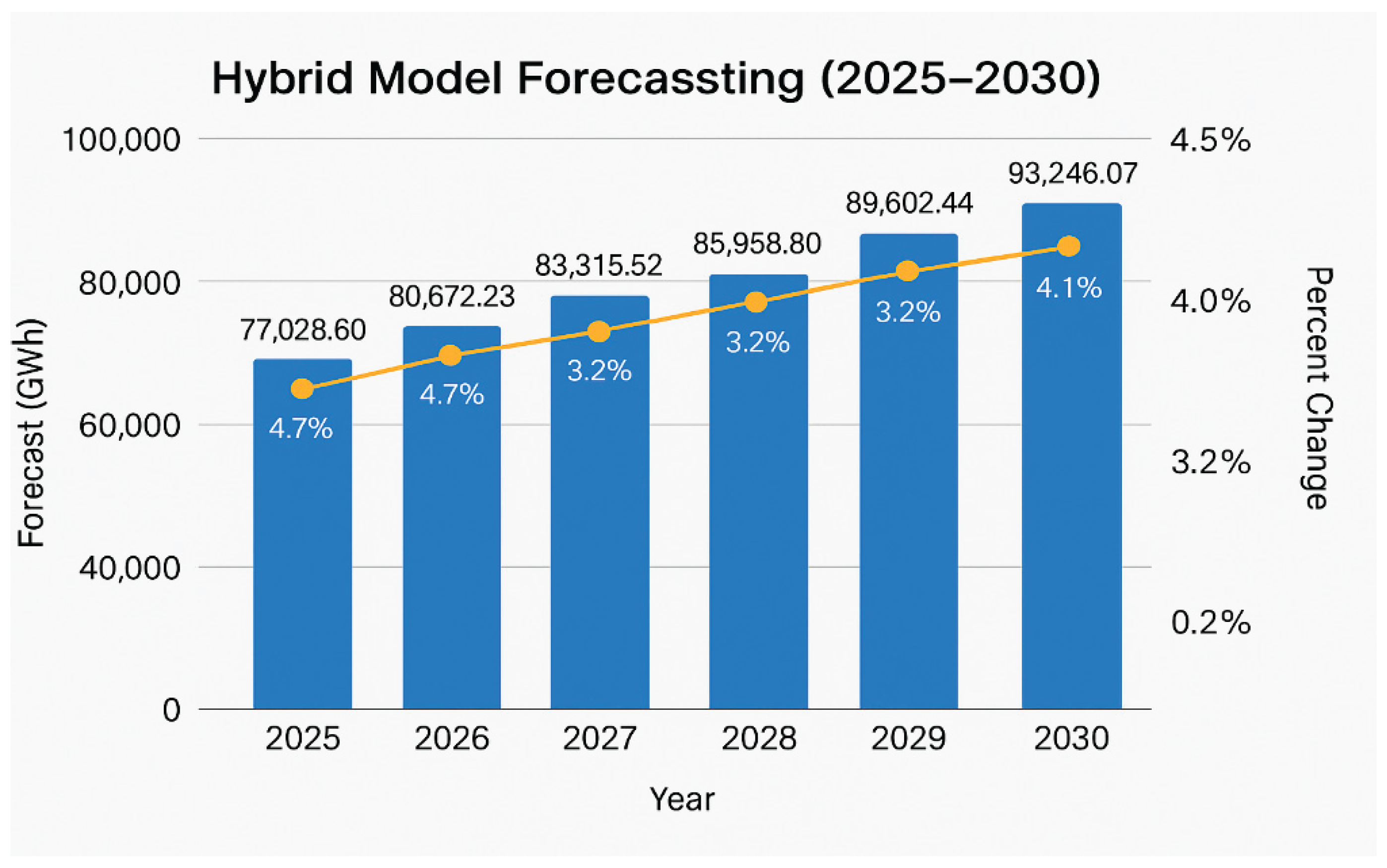
- When the forecast method was rerun by combining the Lasso and Random Forest models in the hybrid model to achieve optimal results, the following energy consumption estimates were generated: 77028.59 GWH for 2025, 80672.22 GWH for 2026, 83315.51 GWH for 2027, 85598 GWH for 2028, 85958 GWH for 2029, and 93246.07 GWH for 2030. These values are demonstrated in Figure 3.
Figure 3.
Hybrid Model Forecasting.
- When all results were compared with the hybrid model, Arima, Lasso, and Linear Regression models produced the closest results to the hybrid model. Polynomial and Exponential estimation methods produced the farthest estimates from the hybrid model. This situation is demonstrated in Table 4.
Between 2025 and 2030, consumption estimates increased from 77,028 GWh to 93,246 GWh. Percentage changes of 2% to 4% are observed annually. Additional yearly representations are shown in Figure 4.
In 2025, the ARIMA model produced a 1.56% higher forecast than the Hybrid model. The difference was 1.05% in 2026, 1.00% in 2027, and 0.36% in 2028. However, in 2029 and 2030, ARIMA performed 1.83% and 4.20% lower than the Hybrid model, respectiveLy.
In general, the ARIMA model produced forecasts close to the Hybrid model between 2025 and 2028, but its error increased in 2029 and 2030.
The Exponential method produced significantly higher values than the Hybrid model in all years. The difference was 4.20% in 2025, 6.99% in 2026, 10.83% in 2027, 14.46% in 2028, 16.55% in 2029, and 18.47% in 2030. This reveals that the Exponential method tends to have increased error and performs poorly compared to the Hybrid model. This situation is demonstrated in Figure 4.
The linear model's predictions are almost identical to those of the hybrid model. The differences ranged from 0.01% to 0.03% between 2025 and 2030. This suggests that the linear model yields very similar results to the hybrid model, and that the combined model does not differ significantly from linear regression.
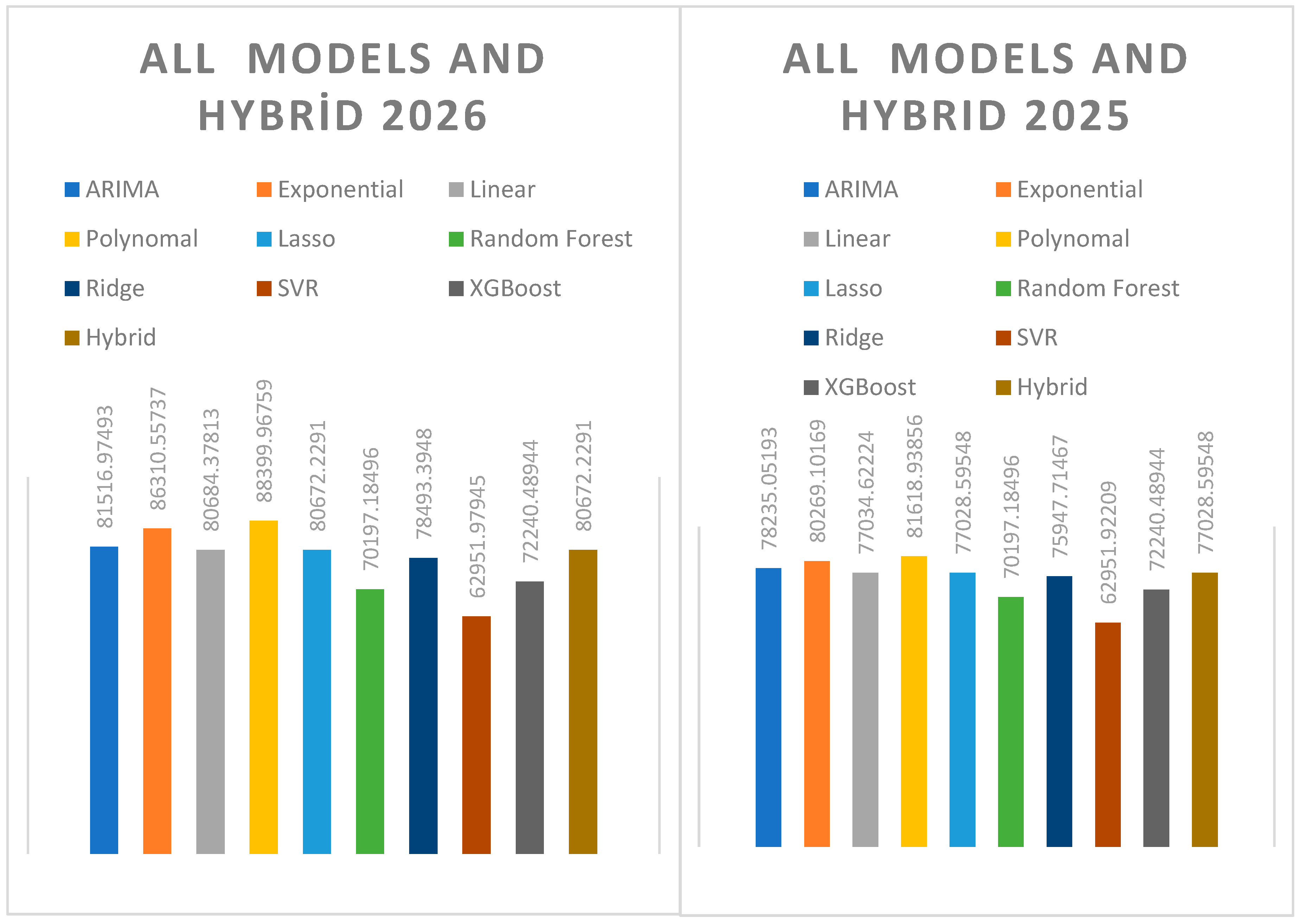
Figure 5.
All Models And Hybrid Model Estimation 2025-2026.
The polynomial model showed a significant overestimation bias compared to the hybrid model in all years. The difference was 5.95% in 2025, 9.58% in 2026, 14.24% in 2027, 18.63% in 2028, 21.40% in 2029, and 23.88% in 2030. The polynomial approach produced high-variance and over-biased forecasts and was one of the methods that yielded the largest overestimations compared to the hybrid model.
The fact that the hybrid model and lasso show very close values indicates that the lasso is used as the dominant estimation in the hybrid model.
The Random Forest model produced lower predictions than the Hybrid model every year. The difference reached 8.86% in 2025, 13.00% in 2026, 17.09% in 2027, 20.78% in 2028, 25.42% in 2029, and 28.93% in 2030.
The SVR model produced a constant value compared to the Hybrid model, yielding the same forecast each year (approximately 62,952 GWh). Between 2025 and 2030, the differences increased by 18.27%, 28.67%, 32.87%, 36.66%, 41.75%, and 48.97%, respectively. The SVR, with its static and underestimation bias, exhibited the weakest performance compared to the Hybrid model.
The XGBoost model underestimated Hybrid in all years, but it was not as stable as SVR. The difference was 6.61% in 2025, 8.59% in 2026, 9.80% in 2027, 7.76% in 2028, 9.56% in 2029, and 10.18% in 2030. XGBoost is a consistent but conservative model, and systematically underestimates Hybrid.
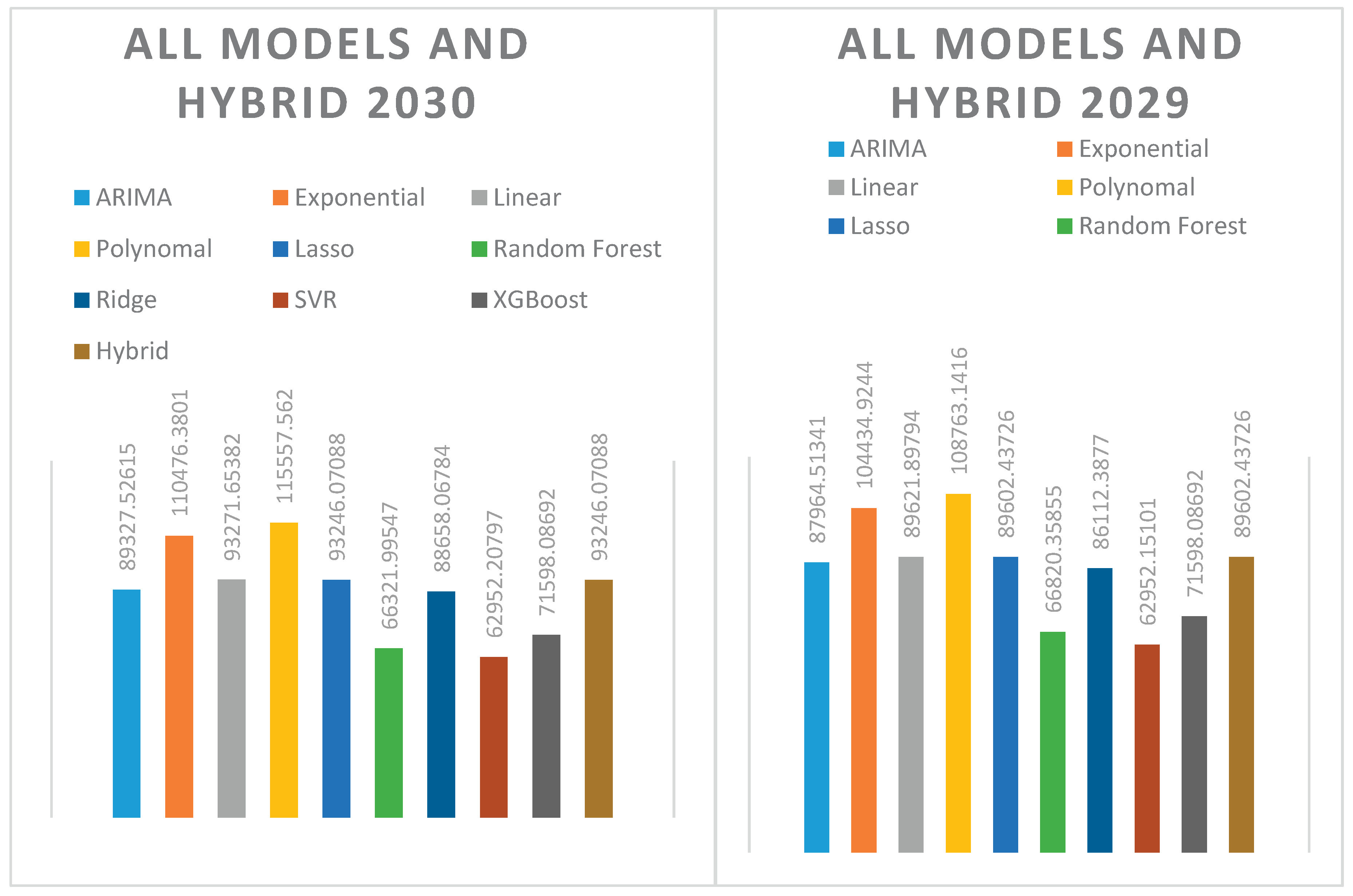
Figure 6.
All Models And Hybrid Model Estimation 2027-2028.

The Ridge model produced lower forecast errors than the Hybrid model in all years. The difference was 1.40% in 2025, 2.78% in 2026, 2.74% in 2027, 2.85% in 2028, 3.89% in 2029, and 5.00% in 2030.
As general results, the closest predictions were determined to be Lasso and Linear Regression, the worst predictions were SVR and Polynomial Regression, the extremely low predictions were determined to be Random Forest, the extremely high predictions were determined to be Polynomial and Exponential, and the consistent but remaining models that did not exceed the accuracy of the Hybrid model were determined to be Ridge and XGBoost.
Correlation Assessment
Figure 7.
All Models And Hybrid Model Estimation 2029-2030.
- The correlation between electricity consumption and gross domestic product was 0.995.
- The correlation between electricity consumption and the number of university graduates was 0.9971.
- The correlation between electricity consumption and population was 0.9827.
This shows that the relationship between GDP and demand is very highly positive, the relationship between the number of university graduates and consumption is strongly positive, and the correlation between population and electricity consumption is highly positive.
Conclusion
In this study, Turkey's wind, solar, and geothermal energy demand for the period 2025–2030 was forecasted using ten different predictive methods, including ARIMA, Exponential Smoothing, Linear Regression, Polynomial Regression, Lasso, Ridge, SVR, Random Forest, XGBoost, and Artificial Neural Networks. The results were then compared with a hybrid forecasting model developed as part of the study. Through backtesting-based analysis, the performance of each model was evaluated annually by comparing absolute and percentage differences with the hybrid model. The effect ratios of the variables affecting the prediction result were determined by the Pearson Correlation analysis method performed in the hybrid prediction model obtained.
The results indicate that the Lasso regression model produced predictions that were exactly equal to the hybrid model in all years. This finding strongly suggests that Lasso plays a dominant role within the hybrid structure. Similarly, the Linear Regression model produced results with minimal differences (less than 0.03%), indicating a strong structural alignment with the hybrid model. The Ridge regression method also showed relatively close alignment, with annual deviations ranging between 1.4% and 5.1%.
In contrast, the Exponential Smoothing and Polynomial Regression models consistently produced higher forecasts than the hybrid model, especially after 2028. In 2030, the Exponential method overestimated demand by 15.6%, while the Polynomial model deviated by 23.8%, indicating a tendency toward overfitting in long-term projections.
Another notable finding is that the Support Vector Regression (SVR) method consistently generated significantly lower forecasts across all years. The difference between SVR and the hybrid model reached 22.3% in 2025 and increased to 47.9% by 2030. Similarly, Random Forest and XGBoost, despite being powerful machine learning algorithms, showed systematic underestimation compared to the hybrid model, with deviations ranging from 10% to 30%. This behavior suggests a tendency toward conservative forecasting in the absence of careful hyperparameter tuning.
The correlation between electricity consumption and gross domestic product was 0.995, The correlation between electricity consumption and the number of university graduates was 0.9971, The correlation between electricity consumption and population was 0.9827. This shows that the relationship between GDP and demand is very highly positive, the relationship between the number of university graduates and consumption is strongly positive, and the correlation between population and electricity consumption is highly positive.
The hybrid model demonstrated strong agreement with regression-based methods, particularly Lasso, Linear Regression, and Ridge, while significant discrepancies were observed with nonparametric and machine learning-based approaches. These findings highlight the importance of carefully selecting hybrid model components and optimizing them through backtesting. This study's methodological comprehensiveness and comparative multi-model evaluation offer both theoretical and practical contributions to the field of energy demand forecasting. Pearson correlation analysis, applied to the developed hybrid forecasting method, was used to observe the effect ratios of the variables used in the model. This aspect distinguishes the study from other studies.
This study presents important findings through a comprehensive comparison of multiple forecasting models and the development of a hybrid approach to forecast Türkiye's wind, solar, and geothermal energy demand. However, some improvements can be made in future research. First, forecasting accuracy can be further enhanced by applying AI-based optimization techniques such as Genetic Algorithms, Grid Search, or Bayesian Optimization to increase accuracy. The backtesting framework can also be extended using advanced techniques such as time-series cross-validation. Furthermore, developing sub-regional models at the city or provincial level and assessing their scalability will increase the practical applicability of the approach. Finally, integrating variables related to energy storage systems, electric vehicle adoption, and green energy policies into the forecasting process can provide more strategic insights for long-term sustainable energy planning.
References
- Dudek, G. Hybrid Residual Dilated LSTM and Exponential Smoothing Method for Medium-Term Electricity Load Forecasting. 2020. [Google Scholar]
- Lee, J.; Cho, Y. National-Scale Electricity Peak Load Forecasting: Traditional, ML, or Hybrid Model? Energy 2022, 239. [Google Scholar] [CrossRef]
- Roy, K.; Maity, S.; Ghosh, P. 2021. Electricity Demand Forecasting in Smart Grid Using Long Short-Term Memory (LSTM).
- Jun, A. 2022. A Hybrid Forecasting Model Using LSTM and Prophet for Energy Consumption with Decomposition of Time Series Data. ResearchGate.
- Doğan, G.Y.; Kaya, F.; Öztürk, A. A Hybrid Deep Learning Model to Estimate the Future Electricity Demand of Sustainable Cities. Sustainability 2024, 16, 6503. [Google Scholar] [CrossRef]
- Li, X.; Zhang, Q.; Chen, M. A Hybrid Forecasting Model for Electricity Demand in Sustainable Power Systems Based on Support Vector Machines. Energies 2024, 17, 4377. [Google Scholar] [CrossRef]
- Ugbehe, P.O.; Dike, T.; Okoro, C.M. Electricity Demand Forecasting Methodologies and Applications: A Review. Sustain. Energy Res. 2025, 14, 1–23. [Google Scholar] [CrossRef]
- Javanmard, M.; Ghaderi, S.F. Energy Demand Forecasting in Seven Sectors in Iran Using ANN, ARIMA, SARIMA and LSTM Models. Energy Strategy Rev. 2023, 42, 101037. [Google Scholar]
- Ashtar, D.; van den Berg, N.; van Aken, M. May Hybrid Multi-Stage Forecasting for Sustainable Electricity Demand Planning in the Netherlands. Preprints.org. 2025.
- Khan, M.A.; Taj, N.R.; Smith, L.E. Short-Term Electricity Demand Forecasting in Smart Homes Using Hybrid CNN-LSTM and CNN-GRU Models. Front. Energy Res. 2024, 12, 1323357. [Google Scholar]
- Wang, T.; Yu, Z.; Zhang, H. Multi-Input LSTM-Based Model for Short-Term Electricity Demand Forecasting Using Weather and Mobility Data. Appl. Energy 2023, 347, 121408. [Google Scholar]
- Nguyen, H.T.; Mohanty, S.P.; Kougianos, E. Electricity Demand Forecasting Using GRU-SVR Hybrid Models. IEEE Internet Things J. 2022, 9, 17588–17597. [Google Scholar]
- Al-Qahtani; Elleithy, K. M.; Alotaibi, F. Optimized Support Vector Regression Using Genetic Algorithms for Power Load Forecasting. IEEE Access 2021, 9, 43322–43331. [Google Scholar]
- Kumar, S.; Ranjan, R.; Tiwari, A. Multi-Stage Demand Forecasting Using Prophet, LSTM, XGBoost. Energies 2023, 16, 1852. [Google Scholar]
- Kim, H.; Jang, S.; Lee, D. Application of Transformer Neural Network in Electricity Load Forecasting. IEEE Trans. Smart Grid 2024, 15, 990–1001. [Google Scholar]
- Arafat, *!!! REPLACE !!!*; Haque, M.I.; Rahman, N. Arafat; Haque, M.I.; Rahman, N. Short-Term Load Forecasting in Industrial Zones Using LSTM. IEEE PES ISGT Conference.
- Sarkar; Roy, R. ; Das, P. Comparative Study of Random Forest and LSTM for Energy Demand Prediction in Smart Cities. J. Clean. Prod. 2022, 356, 131915. [Google Scholar]
- Ahmed, F.S.; Ali, M.M. 2024. Electrical Energy Demand Forecasting Using Time Series in LSTM and CNN-LSTM Models in Deep Learning Applications. ResearchGate.
- Arif, M.; Hussain, M. Energy Demand Forecasting and Optimizing Electric Systems for Developing Countries. Int. J. Energy Econ. Policy 2023, 13, 28–35. [Google Scholar]
- Sharma, F.; Verma, A. Performance Comparison of ARIMA, LSTM, SVM in Electricity Demand Forecasting. PreDatecs J. 2023, 7, 42–49. [Google Scholar]
- Zhang, L.; Zhou, Q. Forecasting Peak Energy Demand in Smart Buildings Using ANN and ARIMA Models. J. Supercomput. 2020, 76, 5894–5912. [Google Scholar]
- Park, S.H.; Kim, J. Energy Forecasting in Smart Grid Systems: A Review. arXiv arXiv:2011.12598, 2020. [CrossRef]
- Doğan, G.Y. Electricity Demand Forecasting Using Hybrid CNN-LSTM for City-Level Smart Grid Applications. Energies 2024, 16, 6503. [Google Scholar]
- Bashir, S.; Hussain, A. 2024. Energy Demand Forecasting Using Time Series in LSTM and CNN-LSTM Models. ResearchGate.
- Chen, L.; Han, M.; Xu, Y. Electricity Demand Forecasting in Smart Grid Using SVM and LSTM Models. IEEE Trans. Ind. Inform. 2022, 18, 6934–6942. [Google Scholar]
- Mehmood, R.; Iqbal, U. Deep Learning Based Short-Term Load Forecasting: A Hybrid LSTM-CNN Model. J. Electr. Syst. Inf. Technol. 2022, 9, 10. [Google Scholar]
- Yılmaz, H. Comparison of Artificial Neural Networks and ARIMA Methods in Electricity Demand Forecasting in Turkey. Gazi Univ. J. Sci. 2023, 37, 101–112. [Google Scholar]
- Akçay, N.; Altuğ, F. Performance Comparison of LSTM and Prophet Models in Electricity Demand Forecasting. J. Eng. Sci. 2024, 31, 65–73. [Google Scholar]
- Kaya, T.; Kocak, M. A Hybrid Method Application for Energy Demand Forecasting: The Case of Turkey. Journal of Electrical, Electronics and Computer Sciences 2023, 11, 101–109. [Google Scholar]
- Demirtaş, E.; Şahin, R. Comparative Electricity Demand Forecasting Performance of LSTM and RF Methods. Yıldız Tech. Univ. J. Energy Syst. 2024, 5, 45–54. [Google Scholar]
- Wang, Z.; Li, D. Short-term load forecasting based on ARIMA model. Energy Rep. 2020, 6, 101–106. [Google Scholar]
- Alwee, R.; Yusof, S.; Ismail, N. Electricity consumption forecasting using exponential smoothing methods. Energy Procedia 2014, 62, 512–521. [Google Scholar]
- Mohamed, S.; Kamel, S. Comparison of artificial neural network and linear regression model in electricity demand forecasting. Int. J. Electr. Power Energy Syst. 2015, 67, 562–568. [Google Scholar]
- Şahin, M.; Karabacak, B. Forecasting energy consumption using polynomial regression: A case study for Turkey. Renew. Sustain. Energy Rev. 2018, 82, 2587–2599. [Google Scholar]
- Zhang, X.; Zhou, Y.; Chen, S. Comparative study of Lasso and Ridge Regression in energy consumption modeling. Appl. Energy 2020, 259, 114–122. [Google Scholar]
- Khosravi, H.; Ghadimi, M.; Dehghanian, M.Z. Short-term electricity demand forecasting using random forest. Energy 2019, 182, 543–552. [Google Scholar]
- Ahmad, T.; Chen, H. Short and medium-term forecasting using SVR model for power system load. Appl. Energy 2017, 195, 693–704. [Google Scholar]
- Liu, L.; Wang, K.; Zhang, Y. A novel XGBoost-based model for electricity consumption prediction. Energy 2019, 189, Art. [Google Scholar]
- Deb; Zhang, F. ; Lee, S.E. A review on time series forecasting techniques for building energy consumption. Renew. Sustain. Energy Rev. 2017, 74, 902–924. [Google Scholar] [CrossRef]
- Zarandi, M.H.F.; Hosseini, S.S.; Turksen, H. Electricity load forecasting using hybrid ARIMA and XGBoost model. Energy Build. 2020, 210, Art. [Google Scholar]
Figure 1.
Study Methodology Flow Diagram.
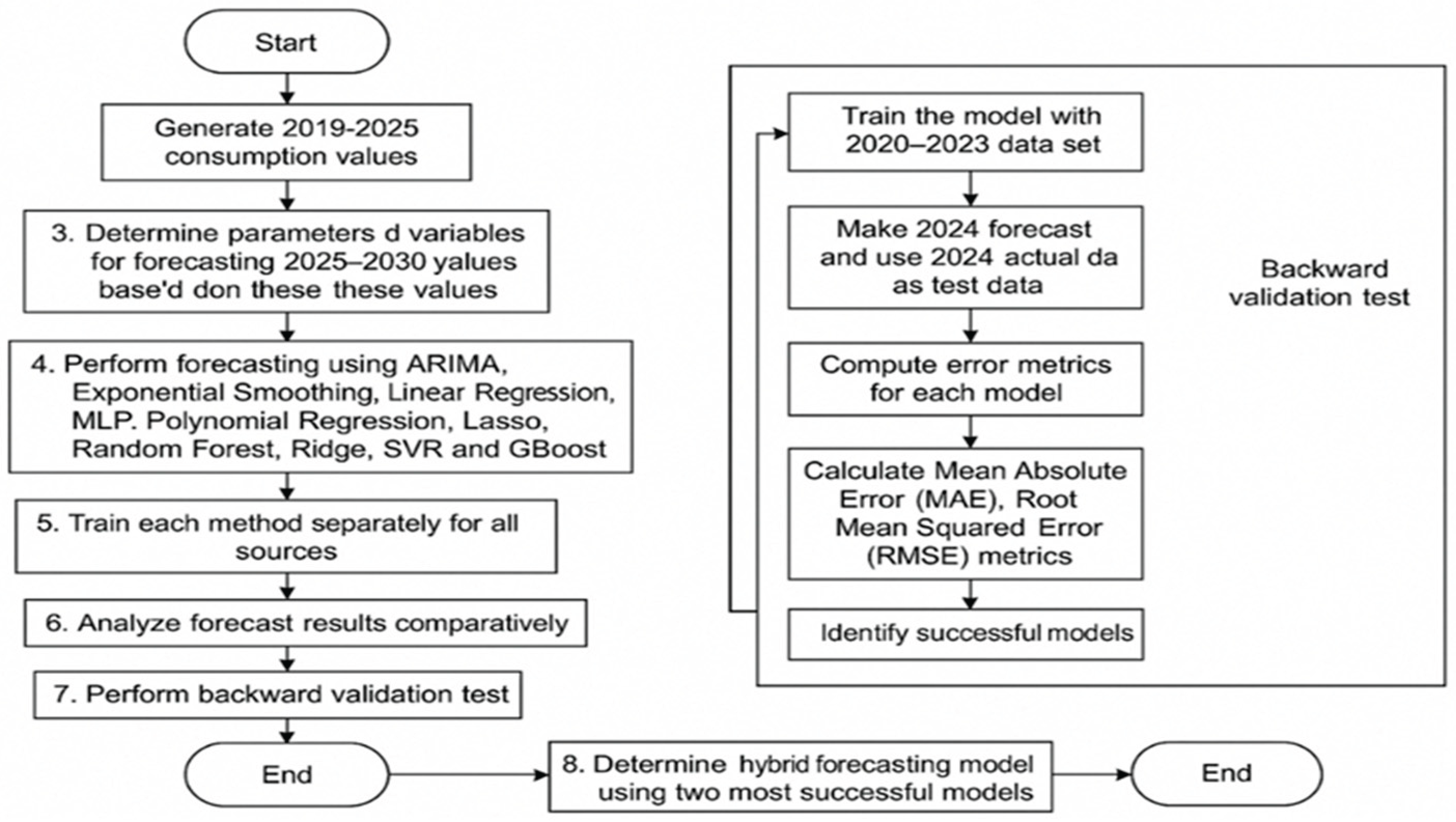
Figure 4.
Hybrid Model Forecasting Annual Change.
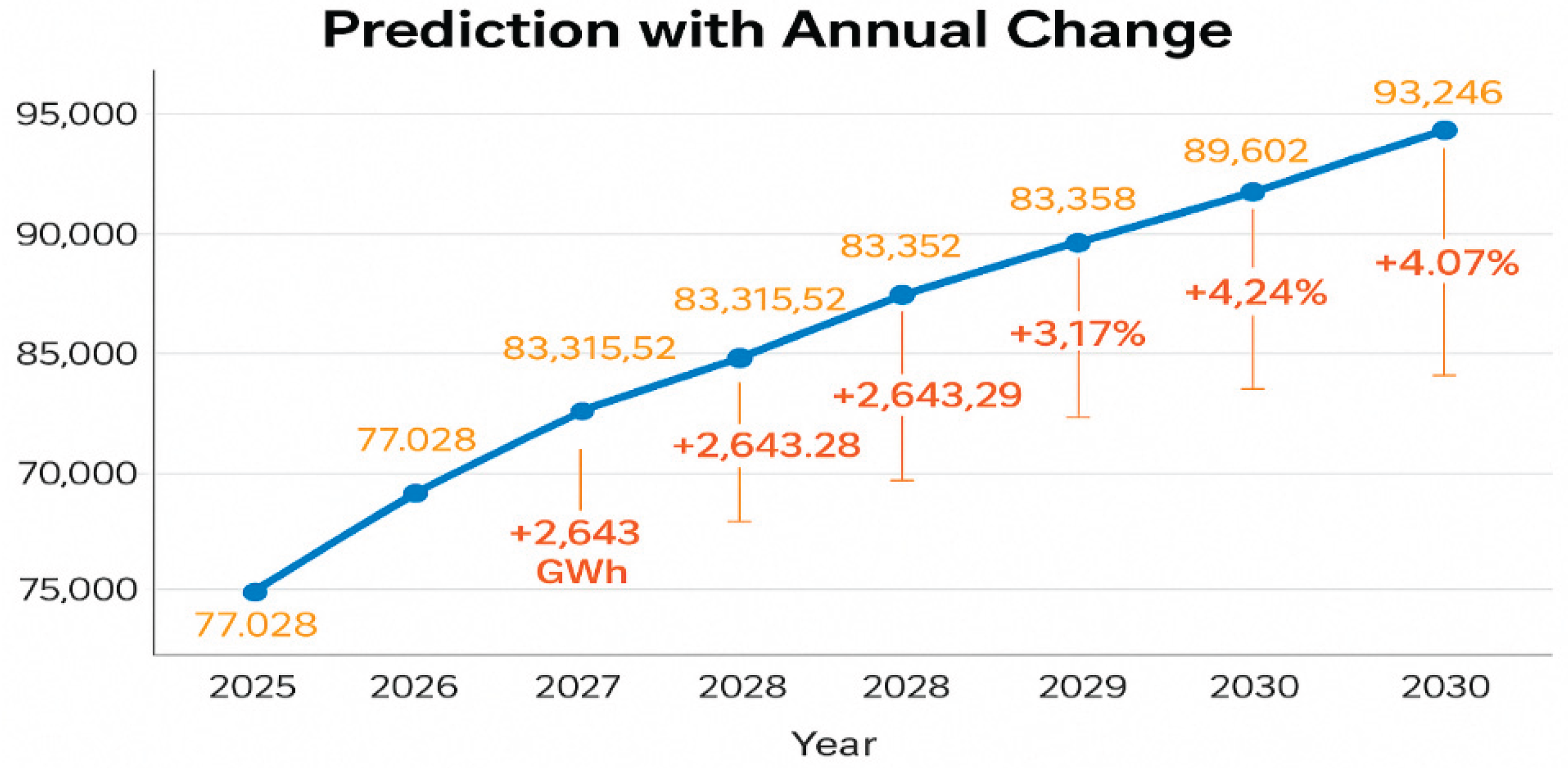

Table 1.
Trained Parameters.
| Parameter | Estimated Value | Description |
|---|---|---|
| ϕ1 | 0.88 | AR coefficient with 1st lag |
| ϕ2 | -0.15 | AR coefficient with 2nd lag |
| θ1 | 0.43 | MA coefficient |
| c | 320 | Constant Value |
| σ2 | 16,1 | Error Variance |
Table 2.
Forecasting Results.
| Year | ARIMA | Exponential | Linear | Polynomal | Lasso | Random Forest | Ridge | SVR | XGBoost |
|---|---|---|---|---|---|---|---|---|---|
| 2025 | 78235,05193 | 80269,10169 | 77034,62224 | 81618,93856 | 77028,595 | 70197,18496 | 75947,7147 | 62951,9221 | 72240,49 |
| 2026 | 81516,97493 | 86310,55737 | 80684,37813 | 88399,96759 | 80672,229 | 70197,18496 | 78493,3948 | 62951,9794 | 72240,49 |
| 2027 | 84151,61485 | 92352,01304 | 83328,26009 | 95184,34444 | 83315,516 | 69077,68442 | 81030,0512 | 62952,0367 | 72240,49 |
| 2028 | 86266,63325 | 98393,46872 | 85972,14206 | 101972,0691 | 85958,804 | 68095,7602 | 83566,7076 | 62952,0939 | 71598,09 |
| 2029 | 87964,51341 | 104434,9244 | 89621,89794 | 108763,1416 | 89602,437 | 66820,35855 | 86112,3877 | 62952,151 | 71598,09 |
| 2030 | 89327,52615 | 110476,3801 | 93271,65382 | 115557,562 | 93246,071 | 66321,99547 | 88658,0678 | 62952,208 | 71598,09 |
Table 3.
Backtesting Results.
| Model | Year | MAE (GWh) | RMSE (GWh) |
|---|---|---|---|
| Lasso | 2023 | 19,69 | 19,69 |
| Random Forest | 2023 | 4,705 | 4,705 |
| Lasso | 2024 | 6,49 | 6,49 |
| Random Forest | 2024 | 5,698 | 5,698 |
Table 4.
Comparison table of all forecasting methods and the hybrid forecasting method.
| Year | Arima | Exponential | Linear | Polynomal | Lasso | Random Forest | Ridge | SVR | XGBoost | Hybrid |
|---|---|---|---|---|---|---|---|---|---|---|
| 2025 | 78235,05193 | 80269,10169 | 77034,62224 | 81618,93856 | 77028,595 | 70197,18496 | 75947,7147 | 62951,9221 | 72240,49 | 77028,6 |
| 2026 | 81516,97493 | 86310,55737 | 80684,37813 | 88399,96759 | 80672,229 | 70197,18496 | 78493,3948 | 62951,9794 | 73740,49 | 80672,23 |
| 2027 | 84151,61485 | 92352,01304 | 83328,26009 | 95184,34444 | 83315,516 | 69077,68442 | 81030,0512 | 62952,0367 | 76220,49 | 83315,52 |
| 2028 | 86266,63325 | 98393,46872 | 85972,14206 | 101972,0691 | 85958,804 | 68095,7602 | 83566,7076 | 62952,0939 | 79678,09 | 85958,8 |
| 2029 | 87964,51341 | 104434,9244 | 89621,89794 | 108763,1416 | 89602,437 | 66820,35855 | 86112,3877 | 62952,151 | 81598,09 | 89602,44 |
| 2030 | 89327,52615 | 110476,3801 | 93271,65382 | 115557,562 | 93246,071 | 66321,99547 | 88658,0678 | 62952,208 | 83798,09 | 93246,07 |
Disclaimer/Publisher’s Note: The statements, opinions and data contained in all publications are solely those of the individual author(s) and contributor(s) and not of MDPI and/or the editor(s). MDPI and/or the editor(s) disclaim responsibility for any injury to people or property resulting from any ideas, methods, instructions or products referred to in the content. |
© 2025 by the authors. Licensee MDPI, Basel, Switzerland. This article is an open access article distributed under the terms and conditions of the Creative Commons Attribution (CC BY) license (http://creativecommons.org/licenses/by/4.0/).
Copyright: This open access article is published under a Creative Commons CC BY 4.0 license, which permit the free download, distribution, and reuse, provided that the author and preprint are cited in any reuse.


