
Submitted:
14 August 2025
Posted:
14 August 2025
You are already at the latest version
Abstract
Rainfall intensity‒duration‒frequency (IDF) curves are essential for hydrological design and flood management, yet their development in Uganda is limited by scarce subdaily rainfall data. This research regionalized the IDF coefficients using physical and climatic predictors. IDF coefficients (a, b, c) were derived from observed hourly rainfall and from disaggregated daily rainfall using aligned time distribution (TD) factors. The aligned TD method produced consistent coefficients (b: 0.404 to 0.65; c: 1.01 to 1.079) with near-perfect R² values, while the empirical method based on observed hourly data exhibited greater variability, the coefficient a ranged from 32.37 at Soroti to 678.54 at Gulu. Multiple regression analysis (MRA) using elevation, mean, and standard deviation as predictors, performed strongly, particularly with disaggregated data (R² > 92% for all coefficients). Validation showed predicted coefficients closely matched actual values, especially coefficients b and c (percentage error within ±10%), though coefficient a exhibited larger deviations. The MRA model, based on observed data, also performed well for coefficients b and c (R² = 97.65% and 96.25%, respectively). This research demonstrates that regionalizing IDF coefficients using MRA is feasible and effective, providing practical tools for estimating design storm intensities in gauged and ungauged catchments, while recommending cautious application beyond the calibration domain.
Keywords:
subdaily rainfall
; Multiple Regression Analysis (MRA)
; design storms
; rainfall disaggregation
; Annual Maximum Series (AMS)
1. Introduction
The Intensity‒duration‒frequency (IDF) curves are critical tools for hydrological and civil engineering applications [1,2,3]. They provide quantitative estimates of rainfall intensities for different storm durations and return periods, enabling the design of urban drainage systems, culverts, and flood mitigation infrastructure [4,5]. Traditionally, IDF curves are constructed using long-term subdaily rainfall records; however, many regions lack sufficient high-resolution data, specifically in Uganda. [6]. This challenge highlights the critical need to regionalize site-specific IDF curve coefficients to enable their application in data-scarce or ungauged regions of Uganda, thereby supporting the effective planning and design of hydrological infrastructure.
Regionalization provides a practical solution to the challenge of limited long-term subdaily rainfall data by establishing empirical relationships between IDF curve coefficients and readily available site-specific variables [1]. These variables include physical and climatological characteristics such as elevation, as well as statistical properties such as the mean and standard deviation of the annual maximum series (AMS) derived from observed daily rainfall or daily remotely sensed rainfall (RSR) datasets. By leveraging the relationships between site-specific IDF coefficients and physical and climatic characteristics, IDF curve coefficients can be extrapolated to ungauged or poorly monitored areas [3], thereby increasing the accuracy of hydrological design and strengthening climate-resilient infrastructure planning.
Over the past few decades, numerous regionalization techniques have been developed and applied across different parts of the world to estimate IDF curves in data-scarce areas. For example, Acosta-Castellanos et al., [3] conducted a study in the department of Boyacá, Colombia, where they employed two regionalization strategies: (i) interpolation of precipitation intensities for various return periods and durations and (ii) interpolation of IDF parameters derived from the Gumbel distribution via maximum likelihood estimation. These methods were implemented in ArcGIS to produce isoline maps, enabling the estimation of IDF curves at ungauged locations throughout the region. Similarly, Alemaw & Chaoka, [1] developed regional IDF curves for Botswana by applying the fuzzy C-means (FCM) clustering algorithm to delineate three homogeneous rainfall regions based on geographic and climatic variables, including latitude, longitude, and elevation. Within each region, empirical IDF models were calibrated via fitted parameters, and a suitable probability distribution model was used to derive regional IDF relationships. In another study, Mahmoudi et al., [2] regionalized rainfall IDF relationships in Iran by clustering stations into hydrologically homogeneous regions via two unsupervised learning algorithms: neural gas (NG) and growing neural gas (GNG) networks. These clusters were based on geographic and rainfall-related attributes such as latitude, longitude, elevation, mean annual precipitation, and maximum daily rainfall. For each region, the most suitable statistical distribution was selected, and regional IDF curves were developed via the L-moments approach.
In Uganda, research on IDF curve development has focused largely on a few urban centers, such as Kampala, Entebbe, and Jinja, which rely on limited subdaily rainfall data. For example, in the study by Mugume & Butler, [7], IDF curves for Kampala were constructed via daily rainfall records, which were disaggregated into shorter durations via regionalized IDF coefficients from earlier studies by Fiddes et al, [8]. These disaggregated estimates were then used to plot the rainfall intensity against duration for various return periods. More recently, Okirya & Du Plessis, [9] developed site-specific IDF curves for several urban locations, including Gulu, Mbarara, Soroti, Jinja, and Fort Portal, via observed subdaily data. While these studies provide valuable tools for localized hydrological planning, their applicability at regional and national scales remains limited, particularly in rural and ungauged areas where sub-daily rainfall observations are absent and overall data coverage is sparse [6].
These limitations in terms of data availability and the limited geographical scope of existing studies underscore the urgent need to regionalize site-specific IDF coefficients across Uganda. Although regionalization has become increasingly relevant, few studies have investigated the potential of leveraging physical and climatic characteristics, such as elevation and statistical properties derived from the AMS, to estimate IDF coefficients across the country’s various climatic zones. Additionally, limited efforts have been made to validate these regionalization approaches. The objectives of this research are intended to address these gaps by developing practical tools in the form of regionalized IDF coefficients to support hydrological infrastructure planning, particularly in data-scarce regions. The main and specific objectives of the research are outlined below.
1.1. Research Objectives
1.1.1. Main Objective
The main objective of this research is to regionalize station-specific IDF curve coefficients for application in both gauged and ungauged catchments across Uganda.
1.1.2. Specific Objectives
The specific objectives are as follows:
- To derive empirical IDF coefficients (a, b, c) for selected rain gauge stations.
- To develop multiple regression analysis (MRA) models that establish relationships between site-specific IDF coefficients and selected physical and climatic variables.
- To validate the accuracy and suitability of the developed MRA models for regional application.
2. Materials and Methods
This methodology describes the process of regionalizing IDF curve coefficients to support hydrological design in both gauged and ungauged catchments in Uganda. It includes preprocessing of rainfall data, derivation of station-specific coefficients from disaggregated sub-daily records, and development of MRA models. These models relate the coefficients to key physical and climatic variables, with defined procedures for model construction, validation, and performance evaluation.
2.1. Description of the Study Area
Uganda is in East Africa (Figure 1), lies astride the equator, and is characterized by diverse topography and climatic conditions [10,11]. Its landscape features central plateaus, highland ranges in the southwest (such as the Rwenzori Mountains) and east (including Mount Elgon), and lowland plains in the north and along the Albertine Rift [12,13]. Uganda's rainfall regime is governed primarily by the movement of the Intertropical Convergence Zone (ITCZ), a belt of low pressure that migrates seasonally across the equator, influencing convectional rainfall [11,12]. As a result, most parts of the country experience a bimodal rainfall pattern, with two distinct wet seasons typically occurring from March to May and September to November. However, this pattern varies regionally, with some northern areas experiencing a more unimodal distribution, marked by a single prolonged rainy season [14].
2.2. Description of Research Data
2.2.1. Observed Rainfall Data
The observed daily rainfall data used in this research span the period from January 1, 1991, to December 31, 2020, and were collected from eight stations, as shown in Figure 1. Daily rainfall records from six stations, Gulu, Soroti, Arua, Jinja, Fort Portal, and Mbarara, were previously quality controlled and preprocessed in earlier studies by Okirya and Du Plessis [15,16]. Additional daily rainfall data for Entebbe and Tororo, covering the same 1991–2020 period, were similarly quality checked and processed following the methodology described in those prior studies. These daily rainfall datasets were used to extract the AMS, from which the mean and standard deviation were computed. The daily rainfall data for Arua, Entebbe, and Tororo were disaggregated into subdaily hourly values via aligned TD factors, enabling the estimation of IDF curve coefficients.
The research also utilized observed subdaily rainfall data. Subdaily records for five stations, Gulu, Soroti, Fort Portal, Jinja, and Mbarara, were processed and quality controlled in earlier research by Okirya and Du Plessis [17]. Additional subdaily rainfall data from the Arua, Entebbe, and Tororo stations were quality controlled via the same procedure outlined in previous research by Okirya & Du Plessis, [15,16,17]. These newer datasets consisted of complete hourly records for their respective periods: Entebbe (17 September 2023 to 25 July 2025), Arua (26 September 2020 to 4 December 2023), and Tororo (20 December 2021 to 2 November 2023). The subdaily rainfall data from all stations were then used to derive station-specific IDF curve coefficients.
2.2.2. Elevation Data
Elevation data, expressed in meters above sea level, were used in this research as a key predictor to represent topographic influence. The Elevation was included as a key predictor in the development of the Multilinear Regression Analysis (MRA) model for regionalizing IDF coefficients because it significantly influences local rainfall dynamics through orographic effects. The data were extracted from the Shuttle Radar Topography Mission (SRTM) digital elevation model (DEM) for Uganda. This open-source DEM, with a spatial resolution of 30 m × 30 m, was downloaded from the Africa GeoPortal on July 29, 2025, via the following link: https://www.africageoportal.com/datasets/rcmrd::uganda-srtm-dem-30-meters/about.
2.3. Research Data Quality Control and Preprocessing
2.3.1. Rainfall Data Quality
The additional rainfall data (both daily and subdaily) collected for this research required quality control and preprocessing. The daily rainfall data contained text entries such as “TR” to indicate trace amounts (rainfall less than 0.05 mm) and exhibited gaps with missing values; Tororo had 2.74% missing data, whereas Entebbe had 5.29% missing data over the 1991–2020 period. Following the quality control procedures outlined in Okirya and Du Plessis [15], the daily datasets were cleaned to remove non-numeric text, and missing rainfall values were gap-filled. Gaps lasting one to four days were filled via linear interpolation, whereas longer gaps of up to 30 days were addressed via the long-term mean approach. This long-term mean method is favoured for its simplicity, efficiency, and ability to preserve historical trends and is generally suitable when fewer than 10% of the total dataset is missing [18]. The subdaily rainfall data were largely clean and complete at the hourly temporal scale. However, an outlier was identified for Tororo station: a 15-minute rainfall value of 305.5 mm was recorded on 26 October 2023, which resulted in an anomalous daily total of 360 mm. This outlier was detected via the interquartile range (IQR) method [19,20] and further confirmed via visual inspection of time series plots. The anomalous value was corrected to 22.34 mm based on the 95th percentile.
2.3.2. Elevation Data Quality
The extracted elevation data were cross-validated against elevation values from the open-source Google Earth Pro tool to ensure consistency and accuracy. Open-source sources were preferred because of their accessibility, free availability and practical use. Elevation data extraction was conducted within the Quantum Geographic Information System (QGIS) environment, which is a free and open-source geographic information system. Using the “Sample Raster Values” function in QGIS, station coordinates stored as a vector shapefile were used as the “input point layer”, and a 30-meter DEM served as the “Raster Layer to Sample”.
2.4. Detailed Methodology
2.4.1. Derivation of IDF Curve Coefficients
The derivation of IDF curve coefficients requires subdaily rainfall data. In this research, two sources of subdaily rainfall were utilized: (i) ground-based observed subdaily rainfall recorded by rain gauge stations and (ii) subdaily rainfall data generated by disaggregating observed daily rainfall via the aligned TD method. The disaggregation using aligned TD factors was previously conducted by Okirya and Du Plessis [17], and the resulting subdaily rainfall data facilitated the estimation of IDF curve coefficients for five stations: Gulu, Soroti, Jinja, Mbarara, and Fort Portal. For the additional stations Arua, Entebbe, and Tororo, the IDF coefficients were developed following a procedure outlined below.
First, observed daily rainfall values at these additional stations were disaggregated into hourly data via aligned TD factors, as outlined in Equation 1. In the second step, the annual maximum rainfall depths, d for each duration, t (ranging from 1 to 24 hours), were converted into rainfall intensities via the formula I = d/t, where I represents the rainfall intensity in millimeters per hour (mm/h). These intensity values formed the basis for constructing the IDF curves. The third step involved fitting a standard empirical IDF model to the duration–intensity data via Equation 2, which relates intensity to duration through empirical coefficients. Finally, the IDF curves were visualized by plotting rainfall intensity against duration, providing a clear representation of the relationship between rainfall magnitude and storm duration.
The daily rainfall data were disaggregated subdaily following Equation 1 [17].
where represents the estimated rainfall for hours, h, represents the observed total daily rainfall, and represents the corresponding TD factor. The aligned TD factors, developed by Okirya and Du Plessis in earlier research, outperformed other disaggregation methods in replicating observed hourly rainfall, as evidenced by lower RMSE values [17]. For the additional stations of Tororo, Arua, and Entebbe, the corresponding TD factors are provided in Table A1, Table A2 and Table A3 in Appendix A. The standard IDF empirical model used is shown in Equation 2 [3,7,21].
where I is the rainfall intensity (mm/h), t is the storm duration (hours), a is the scaling parameter (mm/h), b is the duration offset (hours), and c is the dimensionless shape parameter. The coefficients a, b, and c are empirical parameters estimated from local rainfall data via nonlinear regression analysis. The quality of the model fit was evaluated via the coefficient of determination ().
2.4.2. Selection of Predictors for Regionalization
The regionalization approach was based on spatial and statistical descriptors specific to each station. Initially, a broad range of predictors was considered, including longitude, latitude, elevation, mean and standard deviation of the AMS, and climate zone classification. However, to minimize the risk of overfitting given the limited number of stations, the model was streamlined to retain only three primary continuous predictor variables: elevation, which accounts for topographic influences on rainfall intensity; the mean of the AMS, which represents the central tendency of extreme rainfall events; and the standard deviation, which reflects the variability in annual extremes. Categorical predictors such as climate zone classification were excluded to prevent overparameterization. The AMS mean was computed as the arithmetic average of the annual maximum daily rainfall series, whereas the standard deviation was calculated via Equation 3 [19,22].
where N is the number of annual maxima values, x represents the AMS rainfall values, and represents the mean of the AMS.
2.4.3. Multilinear Regression Analysis
The MRA model approach was chosen for regionalizing IDF curve coefficients in this research because of its interpretability, computational efficiency, and proven effectiveness in hydrological regionalization [23]. MRA establishes clear empirical relationships between IDF coefficients and readily available physical and climatic predictors, enabling a transparent understanding of how each variable influences rainfall extremes [24]. Unlike more complex machine learning methods, which often require large datasets and operate as “black boxes,” MRA provides a simple, replicable framework well-suited to data-scarce regions, allowing practitioners to achieve reliable results with minimal computational resources while maintaining acceptable accuracy [25]. Five stations, Arua, Entebbe, Soroti, Mbarara, and Fort Portal, were used in the development of the MRA model. The MRA model establishes the relationship between the IDF coefficients and selected predictor variables, enabling the estimation of IDF parameters based on site-specific physical and climatic characteristics. Separate regression models were developed for each of the three IDF parameters (a, b, and c) via the general linear form presented in Equation 4 [23]:
where Y represents the target IDF coefficients (a, b, c) being predicted. The predictor variables are represented by the elevation, mean () and standard deviation (s) of the AMS rainfall data. where is the intercept; , , and are the regression coefficients corresponding to each predictor; and ε denotes the error term.
In standard regression analysis, the regression coefficients (β) are typically estimated using the normal equation, which provides a closed-form solution to the least squares problem. The predictor variables are first organized into a matrix X, with each row representing an observation and each column representing a predictor. An additional column of ones is added to account for the intercept term in the model. The dependent variable (e.g., an IDF coefficient such as a) is arranged into a separate vector y. The normal equation (Equation 5) is then applied, which involves transposing X, multiplying it by itself, inverting the resulting square matrix, and then multiplying this inverse by the transposed X and y. The resulting set of coefficients defines the best-fitting linear model for predicting the IDF coefficient from the given predictors. This matrix-based approach to developing the MRA model is described in detail by Maity [23].
where, X is the matrix of predictor variables (including a column of variables to account for the intercept), and is the vector of actual observed values for the IDF coefficient being modelled. This method ensures that the estimated coefficients minimize the sum of the squared residuals between the actual observed and predicted values. The model performance was assessed via the coefficient of determination (R²), which quantifies the proportion of variance in the dependent variable (a, b, and c coefficients) explained by the independent variables (predictor variables). The R² is calculated via Equation 6 [19,25]:
where represents the actual observed value, is the predicted value, is the mean of the actual observed values, and n is the number of observations. A higher R² value indicates a better fit of the model, implying that a greater proportion of the variability in the IDF coefficient is explained by the selected predictors. In addition to the numerical evaluation, scatter plots of observed versus predicted values were generated for each coefficient (a, b, and c) to visually assess the model’s fit, accuracy, and potential bias. These plots provide insight into how closely predictions align with actual values, aiding interpretation of the regression model's reliability.
3.4.4. MRA Model Validation
Three independent stations (Jinja, Tororo, and Gulu) were used to validate the MRA model. The validation was performed via two key error metrics: absolute error (AE) and percentage error (PE). The AE (Equation 7) quantifies the magnitude of deviation between the predicted and actual coefficient values, offering a straightforward measure of prediction error in the same units as the coefficients. Moreover, PE expresses this deviation as a percentage of the actual value, making it especially useful when comparing performance across coefficients of varying scales (e.g., large values versus smaller b or c values) (Maity, 2018). Together, AE and PE help evaluate how well the MRA model generalizes to new stations by indicating both the size and relative importance of the prediction errors.
The PE was estimated via Equation 8 [19].
where and are the observed and predicted IDF coefficients, respectively.
3. Results
This section presents the IDF coefficients for the additional stations, Entebbe, Arua, and Tororo, along with their elevations and the mean and standard deviation of the AMS. Furthermore, two MRA models are presented: one developed using ground-based observed hourly rainfall data and the other using hourly rainfall generated by applying aligned TD factors to observed daily rainfall. The aligned TD factors, along with the TD factors from other disaggregation methods, are provided in Table A1, Table A2 and Table A3 in the appendix section for reference. Finally, this section provides the results from the validation of both MRA models at selected validation stations.
3.1. IDF Coefficients and Predictor Variables
3.1.1. The IDF Curve Coefficients
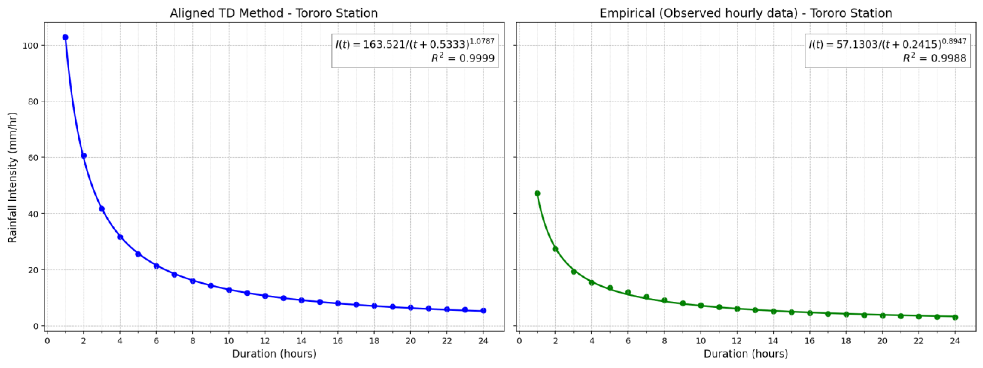
The results in Table 1 show the IDF curve coefficients (a, b, and c) and R² values obtained through two methods: the application of aligned TD factors and empirical fitting to the observed hourly rainfall data. The coefficients for the five stations, Gulu, Soroti, Jinja, Mbarara, and Fort Portal, were derived in our previous study [9]. In this study, those same coefficients are presented in Table 1, alongside newly derived coefficients for three additional stations: Entebbe, Tororo, and Arua. The coefficients derived via the aligned TD method are generally smoother and more consistent, with R² values approaching 100% across all stations. In contrast, the empirical coefficients from the observed hourly data exhibit greater variability, particularly for coefficient a, which ranges from 32.37 at Soroti to 678.54 at Gulu. Coefficient b also shows significant variation, from 0.01 at Soroti to 3.25 at Gulu, whereas the c values vary within a narrower range. Despite this variability, the empirical method still achieves high R² values (97.15–99.95%). Graphical representations of the IDF coefficients and their respective goodness-of-fit (R²) values for the additional stations, Arua, Entebbe, and Tororo, are provided in Figure B1, Figure B2 and Figure B3 in Appendix B section for reference.
3.1.2. Predictor Variables
The results in Table 2 indicate substantial geographical diversity in the elevation predictor, ranging from 1,111 m at Gulu to 1,531 m at Fort Portal. The mean AMS rainfall values ranged from 54.49 mm at Fort Portal to 87.57 mm at Entebbe, highlighting spatial variations in rainfall patterns shaped by location and topography. The standard deviation of the AMS, reflecting rainfall variability, is highest at Entebbe (25.30 mm) and Tororo (21.02 mm), whereas Fort Portal (14.21 mm) has the most stable AMS rainfall patterns.
3.2. MRA Model Development Results
3.2.1. MRA Model Developed Based on Observed Hourly Rainfall Data
The MRA model developed using observed subdaily rainfall data demonstrated varying levels of predictive accuracy for the IDF curve coefficients. The model achieved strong performance for coefficients b and c, with R² values of 97.65% and 96.25%, respectively (Table 3 and Figure 2). However, the model showed relatively lower accuracy for coefficient a, with an R² value of 69.73%.
The graphical results of the MRA model in Figure 2 show that the predictive performance varies across the three IDF coefficients. Coefficient a exhibits moderate accuracy with wider scatter around the 1:1 line, suggesting greater variability in predictions. In contrast, coefficients b and c demonstrate excellent predictive accuracy, with data points closely aligning with the 1:1 reference line. This indicates that the model performs significantly better in estimating b and c than a does, making it more reliable for these parameters in regionalization applications.
3.2.2. MRA Model Based on Disaggregated Rainfall Data
Table 4 presents the results of the MRA model developed via IDF curve coefficients derived from hourly rainfall data generated through the disaggregation of daily observations. The model showed strong predictive accuracy, with coefficient a (R² = 99.92%), coefficients b (R² = 92.81%) and c (R² = 99.84%).
Figure 3 shows scatter plots illustrating the performance of the MRA model in predicting the IDF coefficients a, b, and c. The model demonstrates exceptional predictive performance for coefficients a and c, with the data points almost perfectly aligned along the 1:1 reference line. Coefficient b is slightly lower but still strongly accurate, with a minor scatter around the 1:1 line.
3.3. Validation of the MRA Model
3.3.1. MRA Model Based on Observed Data
The validation results of the MRA model developed from observed subdaily rainfall data revealed mixed performance across the three test stations of Jinja, Gulu, and Tororo (Table 5). While the model showed moderate accuracy at Jinja, with PE ranging from -23.7% to 19.2%, its performance at Gulu was poor, particularly for coefficient a, which was underestimated by 93.71%. Tororo exhibited high overestimation errors, with coefficient a being overpredicted by 86.68% and coefficient b being overpredicted by 218.44%, indicating significant model limitations. These results suggest that the MRA model struggles to generalize well when applied beyond its calibration range, especially for coefficient a, and emphasize the need for improved model calibration or the inclusion of additional predictor variables to enhance robustness across diverse climatic conditions.
3.3.2. MRA Model Based on Disaggregated Rainfall Data
Table 6 presents the validation results of the MRA model developed using data derived from the aligned TD disaggregation method. The results show that the MRA model generally achieved good accuracy for coefficients b and c across Jinja, Gulu, and Tororo, with percentage errors (PEs) mostly within ±11.22%. For coefficient a, performance was more variable, with moderate overestimation at Jinja (PE = 7.75%), significant overestimation at Gulu (PE = 33.15%), and slight underestimation at Tororo (PE = -2.63%). These results indicate the model’s reliability for predicting b and c, while highlighting the need for improvement in estimating a, especially at stations with larger deviations such as Gulu.
4. Discussion
4.1. IDF Curve Coefficients
The comparison of IDF coefficients derived from the application of aligned TD factors and those obtained empirically from observed hourly rainfall data revealed both consistency and variability across stations. The coefficients generated via the aligned TD method are generally more uniform, indicating that a standardized estimation is suitable for regional application. In contrast, empirical coefficients derived from observed hourly data exhibit greater variability, particularly for parameters a and b, with stations such as Gulu and Soroti showing extreme differences. Gulu has notably high values (a = 678.54, b = 3.25), indicating more intense and less frequent storm events, whereas Soroti has much lower values (a = 32.37, b = 0.01), suggesting a drier climate. These findings are consistent with previous work by Okirya and Du Plessis [15], who reported significant seasonal rainfall increases in Gulu, whereas Soroti showed only minor increases, particularly during the September October November (SON) season. Such variability reflects the influence of localized rainfall intensity and temporal distribution patterns. The practical implication is that the aligned TD-based method provides a more standardized approach suitable for regionalization and application in data-scarce areas, whereas empirical methods based on observed data, although potentially more accurate at a given site, may not generalize well owing to their high sensitivity to local rainfall dynamics.
5.2. MRA Model Development Results
The performance of the MRA model in predicting IDF coefficients from observed subdaily rainfall data was generally strong, although it varied across the three coefficients. For coefficient a, the model achieved a moderate coefficient of determination (R²) of 69.7%, whereas coefficient b exhibited excellent performance, with an R² of 97.7%. Similarly, coefficient c yielded a high R² of 96.2%, indicating strong model reliability. When applied to coefficients derived via aligned TD factors, the MRA model performed even better, achieving R² values of 99.9% for a, 92.8% for b, and 99.8% for c, with predicted values closely matching the observed data, especially for a and c. Although predictions for b showed slightly greater dispersion, the correlation remained strong, reaffirming the effectiveness of the MRA model when it was applied to disaggregated datasets. These findings are consistent with earlier studies highlighting the effectiveness of using physical and climatological variables in regionalizing IDF curves [3,24]. The high predictive accuracy for coefficients b and c across both observed and disaggregated data sources suggests that regionalization of IDF curves in ungauged areas is feasible when a limited set of predictors, such as elevation, AMS mean, and standard deviation, is used. This is especially valuable in data-scarce regions where long-term subdaily records are unavailable. Furthermore, the improved predictability of coefficient a under the aligned TD method indicates reduced data noise and improved consistency, which are critical for dependable hydrological design. Therefore, the proposed MRA framework presents a scalable, interpretable, and cost-effective approach for estimating IDF parameters in tropical regions, thereby supporting hydrological infrastructure development and planning in data-scarce tropical settings [1,3].
5.3. Validation of the MRA Model
The validation results of the MRA model based on observed hourly rainfall data revealed mixed predictive performance across stations based on PE estimates. For example, at Jinja, the model performed moderately well, underestimating coefficient a by 23.7% and overestimating b and c by 19.2% and 15.85%, respectively. In contrast, the performance at Gulu was poor: a was underestimated by 93.71%, b was predicted as negative with a −102.43% error, and c was underestimated by 46.53%, indicating that Gulu likely falls outside the model’s calibration range or exhibits distinct rainfall patterns not captured by the predictors. These inconsistencies, especially for a and b, highlight the limited generalizability of the model developed from observed data. In contrast, the model based on the aligned TD factor-derived data yielded more consistent and accurate predictions across all three stations. For instance, for coefficient a, the errors ranged from −2.63% at Tororo to 33.15% at Gulu, with Jinja at 7.75%. The predictions of b were stable and within acceptable limits, with errors between 2.78% (Tororo) and 11.22% (Jinja), and for c, all stations recorded errors below ±3.3%. The observed data-based model showed high variability and major errors at Gulu and Tororo, limiting its reliability for ungauged areas. In contrast, the aligned TD-based model (Table 4) demonstrated consistent performance, especially for b and c, which are key to defining the slope and shape of IDF curves. This makes the aligned TD disaggregation approach more suitable for regionalization and hydrological design in data-scarce environments.
5. Conclusions and Recommendations
5.1. Conclusions
This research aimed to regionalize site-specific IDF curve coefficients for Uganda via both observed subdaily and disaggregated rainfall data. To achieve this goal, (MRA) models were developed using physical and climatic variables, offering a practical tool for estimating design storm intensities in gauged and ungauged catchments to support hydrological infrastructure planning and design efforts.
The research addressed the first specific objective by deriving empirical IDF coefficients (a, b, and c) for additional stations with observed subdaily data and disaggregated long-term observed daily rainfall data. The IDF coefficients derived from aligned TD factors and those obtained empirically from observed hourly rainfall highlight the trade-off between standardization and local specificity. The aligned TD method yields more consistent coefficients across stations, making it suitable for regional applications and ungauged areas. In contrast, the empirically derived coefficients capture local rainfall dynamics more accurately but exhibit high variability, particularly for parameters a and b. This variability, as observed at stations such as Gulu, with coefficients ranging from 32.37 to 678.54, underscores the influence of localized climatic conditions on extreme rainfall characteristics. This spatial variability is consistent with earlier studies by Onyutha and Obubu [13,26] that noted the influence of localized climatic and physiographic factors on rainfall extremes. Therefore, while empirical methods offer site-specific accuracy, the aligned TD approach provides a more reliable and scalable solution for hydrological modelling and infrastructure planning across diverse climatic zones.
To address the second specific objective, MRA models were developed to relate IDF curve coefficients to physical and climatic variables such as elevation, mean AMS rainfall, and AMS standard deviation. Two models were constructed: one using coefficients from observed hourly data and another from disaggregated daily data via aligned TD factors. The MRA model demonstrated strong performance in predicting IDF curve coefficients, with particularly high accuracy for coefficients b and c, and moderate performance for coefficient a when observed subdaily rainfall data were used. The model’s performance improved significantly when it was applied to coefficients derived from aligned TD disaggregation, achieving near-perfect R² values for all three parameters. This highlights the model’s effectiveness and the value of using disaggregated data for regional applications. The findings confirm that a limited set of site-specific predictors, such as elevation, AMS mean, and standard deviation, can effectively support the regionalization of IDF curves, even in ungauged or data-scarce regions [1,3]. Overall, the study validates the MRA framework as a practical, scalable, and cost-effective tool for estimating IDF parameters in tropical settings, with significant implications for hydrological infrastructure planning, design and development.
To address the third specific objective, this research validated the developed MRA models via data from three independent stations, Jinja, Gulu, and Tororo, by comparing the actual and predicted IDF coefficients. The MRA models revealed that while the model based on observed hourly rainfall data demonstrated moderate accuracy at Jinja, it performed poorly at Gulu and inconsistently at Tororo, indicating limited generalizability, especially for coefficients a and b. These limitations suggest that the observed-data-based model may not reliably capture spatial variability in regions with localized rainfall extremes or those lying outside the model’s calibration range. In contrast, the MRA model built using coefficients derived from the aligned TD disaggregation method exhibited markedly better and more consistent performance across all three validation stations. The percentage errors for all the coefficients remained relatively low, particularly for b and c, which are critical for defining the slope and shape of the IDF curve. These findings confirm that the aligned TD approach provides a more stable and transferable basis for regional IDF estimation in both gauged and ungauged areas, making it a more suitable choice for hydrological applications in data-scarce regions.
5.2. Recommendations
Based on the research objectives and findings, the following key recommendations are proposed:
- The aligned TD-based MRA model should be adopted for regional applications, particularly in ungauged or data-scarce catchments. This model demonstrated strong predictive performance, with R² values exceeding 92% and low validation errors across multiple stations, confirming its reliability and suitability for estimating design storm parameters at a regional scale.
- Efforts should be made to improve the availability of subdaily rainfall data by expanding the network of automatic weather stations. The limited accuracy of the MRA model developed from observed IDF coefficients underscores the importance of high-resolution data for improving empirical model calibration and enhancing rainfall intensity estimates.
- Future studies should extend model validation to more stations across different climatic zones in Uganda. This would enhance the model’s generalizability, allow for refinement of regression coefficients, and ensure that the model is robust across the country’s diverse rainfall regimes.
- Given that TD factors for other disaggregation methods have also been developed, such as statistical distribution-based approaches (as presented in Tables 7 to 9 in the annex), future research should explore and compare the performance of these alternative disaggregation techniques. This may help identify the most suitable method for different climatic zones and improve the robustness of the observed subdaily rainfall estimates used in IDF curve development.
- Finally, regionalized IDF models should be incorporated into Uganda’s hydrological and civil engineering design guidelines. Doing so would support the development of more consistent, resilient, and climate-informed stormwater infrastructure, particularly in vulnerable rural and peri-urban areas.
5.3. Research Scope and Limitations
5.3.1. Research Scope
The research scope encompasses the regionalization of IDF curve coefficients via data from eight representative rainfall stations distributed across Uganda’s diverse climatic zones. It utilizes both observed hourly rainfall data and disaggregated daily rainfall data to address data limitations in subdaily records. The daily rainfall data span the period 1991–2020, whereas the observed hourly rainfall data vary in length, ranging from 514 days at Fort Portal to 1,736 days at Mbarara. The research assessed the influence of key spatial and climatic predictors, elevation, and the mean and standard deviation of the AMS, on the estimation of IDF coefficients (a, b, c) MRA models. MRA model development was based on data from five stations, while three additional stations were used to validate the models and assess their predictive performance.
5.3.2. Research Limitations
This research faced several limitations. First, the limited number of stations with long-term, high-quality observed hourly rainfall data may constrain the generalizability and robustness of the regression models. Second, although excluding additional predictors such as land use, proximity to water bodies, and atmospheric circulation patterns helped avoid overfitting, it may have reduced the models' ability to capture the complexity of rainfall variability in diverse terrains and climatic zones. Third, while the aligned TD disaggregation method effectively expands data availability and produces reliable results, testing alternative disaggregation techniques, particularly those based on statistical distribution factors, would provide a broader assessment of model performance. Finally, the validation was limited to a small number of stations; expanding this number in future studies would enhance the nationwide applicability of the developed models.
5.4. Areas for Further Research
Future research should consider building on the contributions of this research to further enhance the regionalization of IDF curve coefficients in Uganda. First, expanding the number of rainfall stations, particularly in underrepresented climatic zones, would improve the spatial coverage and generalizability of the models, while increasing the availability of subdaily data would strengthen model calibration and validation. Second, incorporating additional predictor variables, such as proximity to large water bodies, land use, or regional climate classifications, could enhance the explanatory power of the models, given the complex rainfall-generating mechanisms in tropical regions. Third, future studies should explore advanced modelling techniques such as machine learning (e.g., random forests, support vector regression, or neural networks) and geostatistical approaches, which may offer improved accuracy over traditional MRA methods, particularly in regions with diverse topographies and rainfall variability.
5.5. Novel Contributions
This research makes a novel contribution by developing a scalable and replicable approach for regionalizing IDF curve coefficients in data-scarce environments, with Uganda as the case study. It establishes MRA models that link site-specific IDF coefficients, derived from observed and disaggregated hourly rainfall, to key physical and climatic predictors, including elevation, AMS mean, and AMS standard deviation. Through validation across multiple stations, this research provides a framework for estimating design storm intensities in ungauged areas via readily available inputs such as elevation and daily rainfall data. As such, the proposed MRA model framework serves as a practical and accessible tool for engineers and hydrologists involved in design and hydrological infrastructure planning across Uganda.
Supplementary Materials
The following supporting information can be downloaded at the website of this paper posted on Preprints.org.
Author Contributions
Conceptualization, M.O.; methodology, M.O.; software, M.O.; validation, M.O. and J.D.P.; formal analysis, M.O. and J.D.P.; investigation, M.O. and J.D.P.; resources, M.O. and J.D.P.; data curation, M.O.; writing—original draft preparation, M.O.; writing—review and editing, M.O. and J.D.P.; visualization, M.O. and J.D.P.; supervision, J.D.P.; project administration, J.D.P.; funding acquisition, M.O. and J.D.P. All authors have read and agreed to the published version of the manuscript.
Funding
This research received no external funding.
Data Availability Statement
The Uganda National Meteorological Authority (UNMA) provided the observed daily and subdaily rainfall data. The observed daily rainfall raw data supporting the conclusions of this article will be made available by the authors on request. The 30 m × 30 m DEM for Uganda was downloaded from the Africa GeoPortal on July 29, 2025, via the following link: https://www.africageoportal.com/datasets/rcmrd::uganda-srtm-dem-30-meters/about.
Conflicts of Interest
The authors declare no conflicts of interest.
Abbreviations
The following abbreviations are used in this manuscript:
| AE | Absolute Error |
| AMS | Annual Maximum Series |
| DEM | Digital Elevation Model |
| FCM | Fuzzy C-Means |
| GEV | Generalized Extreme Value |
| GLOG | Generalized Logistic Distribution |
| GNG | Growing Neural Gas |
| IDF | Intensity-Duration-Frequency |
| ITCZ | Intertropical Convergence Zone |
| MRA | Multiple Regression Analysis |
| NG | Neural Gas |
| PE | Percentage Error |
| QGIS | Quantum Geographic Information System |
| RSR | Remotely Sensed Rainfall |
| SON | September-October-November |
| SRTM | Shuttle Radar Topography Mission |
| TD | Time Distribution |
Appendix A

Table A1.
Time distribution factors for Tororo station.
| Hour | Gamma | Weibull | Exponential | Lognormal | GEV | Empirical | Aligned |
| 1 | 0.41 | 0.54 | 0.59 | 0.62 | 0.55 | 0.04 | 0.78 |
| 2 | 0.19 | 0.18 | 0.22 | 0.16 | 0.16 | 0.02 | 0.14 |
| 3 | 0.11 | 0.09 | 0.09 | 0.07 | 0.08 | 0.01 | 0.03 |
| 4 | 0.07 | 0.05 | 0.04 | 0.04 | 0.05 | 0.02 | 0.01 |
| 5 | 0.05 | 0.03 | 0.02 | 0.03 | 0.03 | 0.02 | 0.01 |
| 6 | 0.04 | 0.02 | 0.01 | 0.02 | 0.02 | 0.04 | 0 |
| 7 | 0.03 | 0.02 | 0.01 | 0.01 | 0.02 | 0.01 | 0 |
| 8 | 0.02 | 0.01 | 0 | 0.01 | 0.01 | 0.01 | 0 |
| 9 | 0.02 | 0.01 | 0 | 0.01 | 0.01 | 0.02 | 0 |
| 10 | 0.01 | 0.01 | 0 | 0.01 | 0.01 | 0.01 | 0 |
| 11 | 0.01 | 0.01 | 0 | 0 | 0.01 | 0 | 0 |
| 12 | 0.01 | 0 | 0 | 0 | 0.01 | 0 | 0 |
| 13 | 0.01 | 0 | 0 | 0 | 0.01 | 0 | 0 |
| 14 | 0 | 0 | 0 | 0 | 0.01 | 0.01 | 0 |
| 15 | 0 | 0 | 0 | 0 | 0 | 0.06 | 0 |
| 16 | 0 | 0 | 0 | 0 | 0 | 0.11 | 0 |
| 17 | 0 | 0 | 0 | 0 | 0 | 0.24 | 0 |
| 18 | 0 | 0 | 0 | 0 | 0 | 0.09 | 0.01 |
| 19 | 0 | 0 | 0 | 0 | 0 | 0.1 | 0 |
| 20 | 0 | 0 | 0 | 0 | 0 | 0.07 | 0 |
| 21 | 0 | 0 | 0 | 0 | 0 | 0.03 | 0 |
| 22 | 0 | 0 | 0 | 0 | 0 | 0.05 | 0 |
| 23 | 0 | 0 | 0 | 0 | 0 | 0.03 | 0.01 |
| 24 | 0 | 0 | 0 | 0 | 0 | 0.02 | 0 |
Table A2.
Time distribution factors for Entebbe station.
| Hour | Gamma | Weibull | Exponential | Lognormal | GEV | Empirical | Aligned |
| 1 | 0.39 | 0.51 | 0.54 | 0.57 | 0.54 | 0.02 | 0.70 |
| 2 | 0.19 | 0.18 | 0.22 | 0.16 | 0.16 | 0.04 | 0.15 |
| 3 | 0.11 | 0.09 | 0.10 | 0.08 | 0.08 | 0.05 | 0.06 |
| 4 | 0.07 | 0.06 | 0.05 | 0.05 | 0.05 | 0.05 | 0.03 |
| 5 | 0.05 | 0.04 | 0.03 | 0.03 | 0.03 | 0.06 | 0.02 |
| 6 | 0.04 | 0.03 | 0.02 | 0.02 | 0.02 | 0.15 | 0.01 |
| 7 | 0.03 | 0.02 | 0.01 | 0.02 | 0.02 | 0.09 | 0.01 |
| 8 | 0.02 | 0.01 | 0.01 | 0.01 | 0.01 | 0.10 | 0.00 |
| 9 | 0.02 | 0.01 | 0.00 | 0.01 | 0.01 | 0.09 | 0.00 |
| 10 | 0.01 | 0.01 | 0.00 | 0.01 | 0.01 | 0.11 | 0.00 |
| 11 | 0.01 | 0.01 | 0.00 | 0.01 | 0.01 | 0.07 | 0.00 |
| 12 | 0.01 | 0.01 | 0.00 | 0.01 | 0.01 | 0.07 | 0.00 |
| 13 | 0.01 | 0.01 | 0.00 | 0.00 | 0.01 | 0.03 | 0.00 |
| 14 | 0.01 | 0.00 | 0.00 | 0.00 | 0.01 | 0.02 | 0.00 |
| 15 | 0.01 | 0.00 | 0.00 | 0.00 | 0.01 | 0.02 | 0.00 |
| 16 | 0.00 | 0.00 | 0.00 | 0.00 | 0.00 | 0.02 | 0.00 |
| 17 | 0.00 | 0.00 | 0.00 | 0.00 | 0.00 | 0.02 | 0.00 |
| 18-24 | 0.00 | 0.00 | 0.00 | 0.00 | 0.00 | 0.00 | 0.00 |
Table A3.
Time distribution factors for Arua station.
| Hour | Gamma | Weibull | Exponential | Lognormal | GEV | Empirical | Aligned |
| 1 | 0.40 | 0.51 | 0.56 | 0.57 | 0.53 | 0.05 | 0.74 |
| 2 | 0.19 | 0.18 | 0.22 | 0.16 | 0.16 | 0.05 | 0.14 |
| 3 | 0.11 | 0.09 | 0.10 | 0.08 | 0.08 | 0.04 | 0.03 |
| 4 | 0.07 | 0.05 | 0.05 | 0.05 | 0.05 | 0.07 | 0.03 |
| 5 | 0.05 | 0.04 | 0.03 | 0.03 | 0.03 | 0.09 | 0.01 |
| 6 | 0.04 | 0.03 | 0.02 | 0.02 | 0.02 | 0.04 | 0.01 |
| 7 | 0.03 | 0.02 | 0.01 | 0.02 | 0.02 | 0.04 | 0.01 |
| 8 | 0.02 | 0.01 | 0.01 | 0.01 | 0.02 | 0.03 | 0.00 |
| 9 | 0.02 | 0.01 | 0.00 | 0.01 | 0.01 | 0.02 | 0.00 |
| 10 | 0.01 | 0.01 | 0.00 | 0.01 | 0.01 | 0.02 | 0.00 |
| 11 | 0.01 | 0.01 | 0.00 | 0.01 | 0.01 | 0.01 | 0.00 |
| 12 | 0.01 | 0.01 | 0.00 | 0.01 | 0.01 | 0.01 | 0.00 |
| 13 | 0.01 | 0.01 | 0.00 | 0.00 | 0.01 | 0.02 | 0.00 |
| 14 | 0.01 | 0.00 | 0.00 | 0.00 | 0.01 | 0.04 | 0.00 |
| 15 | 0.00 | 0.00 | 0.00 | 0.00 | 0.01 | 0.03 | 0.00 |
| 16 | 0.00 | 0.00 | 0.00 | 0.00 | 0.01 | 0.05 | 0.00 |
| 17 | 0.00 | 0.00 | 0.00 | 0.00 | 0.00 | 0.05 | 0.00 |
| 18 | 0.00 | 0.00 | 0.00 | 0.00 | 0.00 | 0.03 | 0.00 |
| 19 | 0.00 | 0.00 | 0.00 | 0.00 | 0.00 | 0.07 | 0.01 |
| 20 | 0.00 | 0.00 | 0.00 | 0.00 | 0.00 | 0.08 | 0.01 |
| 21 | 0.00 | 0.00 | 0.00 | 0.00 | 0.00 | 0.04 | 0.00 |
| 22 | 0.00 | 0.00 | 0.00 | 0.00 | 0.00 | 0.03 | 0.00 |
| 23 | 0.00 | 0.00 | 0.00 | 0.00 | 0.00 | 0.06 | 0.00 |
| 24 | 0.00 | 0.00 | 0.00 | 0.00 | 0.00 | 0.03 | 0.00 |
Appendix B
Figure B1.
IDF curves derived from aligned TD factors and hourly rainfall at Arua station.
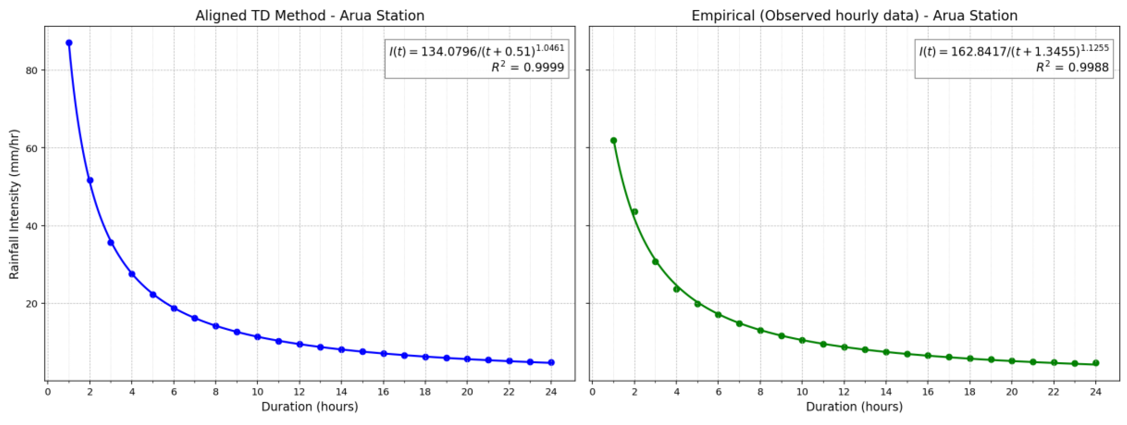
Figure B2.
IDF curves derived from the aligned TD factors and hourly rainfall at Entebbe station.
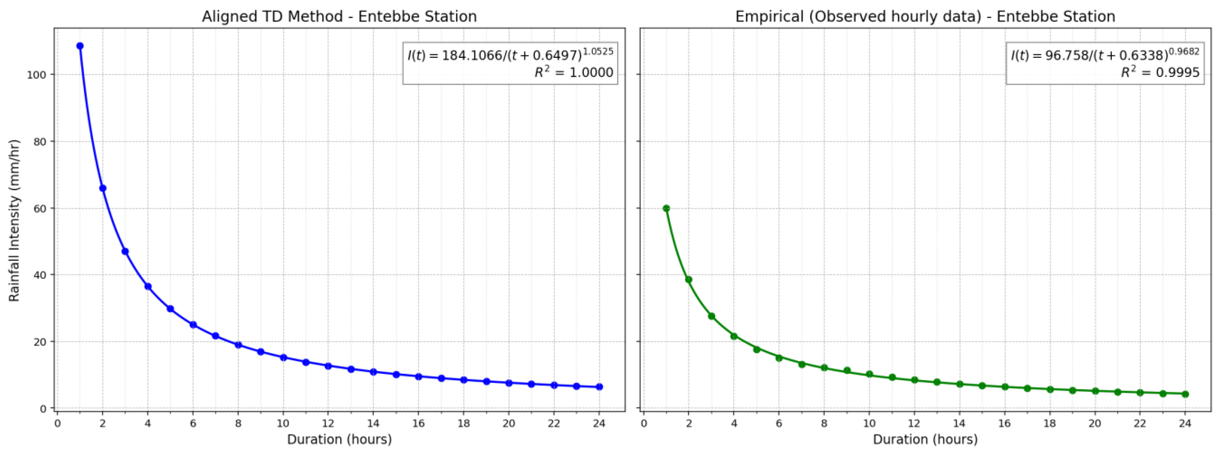
Figure B3.
IDF curves derived from aligned TD factors and hourly rainfall at Tororo station.
References
- B. F. Alemaw and R. T. Chaoka, “Regionalization of Rainfall Intensity-Duration-Frequency (IDF) Curves in Botswana,” J. Water Resour. Prot., vol. 08, no. 12, pp. 1128–1144, 2016. [CrossRef]
- M. R. Mahmoudi, S. Eslamian, S. Soltani, and M. Tahanian, “Regionalization of rainfall intensity–duration–frequency (IDF) curves with L-moments method using neural gas networks,” Theor. Appl. Climatol., vol. 151, no. 1–2, pp. 1–11, 2023. [CrossRef]
- P. M. Acosta-Castellanos, Y. A. C. Ortegón, and N. R. P. Granados, “Regionalization of IDF Curves by Interpolating the Intensity and Adjustment Parameters: Application to Boyacá, Colombia, South America,” Water (Switzerland), 2023. [CrossRef]
- N. M. Ariff, A. A. Jemain, K. Ibrahim, and W. Z. Wan Zin, “IDF relationships using bivariate copula for storm events in Peninsular Malaysia,” J. Hydrol., vol. 470–471, pp. 158–171, 2012. [CrossRef]
- Y. Sun, D. Wendi, D. E. Kim, and S. Y. Liong, “Deriving intensity – duration – frequency ( IDF ) curves using downscaled in situ rainfall assimilated with remote sensing data,” Geosci. Lett., 2019. [CrossRef]
- A. Gahwera and O. Steven, “A Weather Features Dataset for Prediction of Short-term Rainfall Quantities A weather features dataset for prediction of short-term rainfall quantities in Uganda,” Data Br., vol. 50, no. September, p. 109613, 2023. [CrossRef]
- S. N. Mugume and D. Butler, “Evaluation of functional resilience in urban drainage and flood management systems using a global analysis approach,” Urban Water J., vol. 14, no. 7, pp. 727–736, 2017. [CrossRef]
- D. Fiddes, J. A. Forsgate, and A. O. Grigg, “THE PREDICTION OF STORM RAINFALL IN EAST AFRICA,” Crowthorne, Bershire, 1974. Accessed: Apr. 16, 2021. [Online]. Available: https://trid.trb.org/view/21630.
- M. Okirya and J. Du Plessis, “Development of IDF curves for Uganda Using Observed, Remotely Sensed, and Regional Climate Model rainfall data, 02 July 2025, PREPRINT (Version 1) available at Research Square,” 2025. [CrossRef]
- J. G. M. Majaliwa et al., “Characterization of Historical Seasonal and Annual Rainfall and Temperature Trends in Selected Climatological Homogenous Rainfall Zones of Uganda,” Glob. J. Sci. Front. Res., vol. 15, no. 4, pp. 21–40, 2015.
- B. A. Ogwang et al., “Characteristics and changes in SON rainfall over Uganda (1901-2013),” J. Environ. Agric. Sci., vol. 8, no. September 2018, pp. 45–53, 2016, [Online]. Available: https://www.researchgate.net/publication/306324232.
- J. Kisembe, A. Favre, A. Dosio, C. Lennard, G. Sabiiti, and A. Nimusiima, “Evaluation of rainfall simulations over Uganda in CORDEX regional climate models,” Theor. Appl. Climatol., vol. 137, no. 1–2, pp. 1117–1134, 2019. [CrossRef]
- C. Onyutha, “Geospatial trends and decadal anomalies in extreme rainfall over Uganda, East Africa,” Adv. Meteorol., vol. 2016, 2016. [CrossRef]
- World Bank, “Climate Risk Country Profile - Uganda,” 1818 H Street NW, Washington, DC 20433, 2021. [Online]. Available: www.worldbank.org.
- M. Okirya and J. Du Plessis, “Trend and Variability Analysis of Annual Maximum Rainfall Using Observed and Remotely Sensed Data in the Tropical Climate Zones of Uganda,” Sustain., vol. 16, no. 14, 2024. [CrossRef]
- M. Okirya and J. Du Plessis, “Evaluating Bias Correction Methods Using Annual Maximum Series Rainfall Data from Observed and Remotely Sensed Sources in Gauged and Ungauged Catchments in Uganda,” Hydrol., 2025. [CrossRef]
- M. Okirya and J. Du Plessis, “Assessing Rainfall Disaggregation Techniques and Subdaily Rainfall Patterns Across Uganda’s Tropical Climatic Zones, 24 June, PREPRINT (Version 1) available at Research Square,” 2025. [CrossRef]
- A. Chinasho, B. Bedadi, T. Lemma, T. Tana, T. Hordofa, and B. Elias, “Evaluation of Seven Gap-Filling Techniques for Daily Station-Based Rainfall Datasets in South Ethiopia,” Adv. Meteorol., vol. 2021, 2021. [CrossRef]
- R. Maity, Statistical Methods in Hydrology and Hydroclimatology. 2018. [Online]. Available: http://www.springer.com/series/13593.
- C. Zhao and J. Yang, “A Robust Skewed Boxplot for Detecting Outliers in Rainfall Observations in Real-Time Flood Forecasting,” Adv. Meteorol., vol. 2019, pp. 1–7, 2019. [CrossRef]
- N. Wagesho and M. Claire, “Analysis of Rainfall Intensity-Duration-Frequency Relationship for Rwanda,” J. Water Resour. Prot., vol. 8, no. June, pp. 706–723, 2016. [CrossRef]
- S. Andre, G. Abhishek, P. S. Slobodan, and D. Sandink, Computerized Tool for the Development of Intensity-Duration- Frequency Curves Under a Changing Climate, Version 3. London, Ontario, Canada: The University of Western Ontario, Department of Civil and Environmental Engineering and Institute for Catastrophic Loss Reduction, 2018. [Online]. Available: www.idf-cc-uwo.ca.
- R. Maity, Statistical methods in hydrology, Second. Kharagpur, India: Springer Nature Singapore Pte Ltd, 2022. [CrossRef]
- H. Madsen, P. S. Mikkelsen, D. Rosbjerg, and P. Harremoes, “Regional estimation of rainfall intensity-duration-frequency curves using generalized least squares regression of partial duration series statistics,” Water Resour. Res., vol. 38, no. 11, p. 1239, 2002. [CrossRef]
- J. L. Salinas et al., “Comparative assessment of predictions in ungauged basins-Part 2: Flood and low flow studies,” Hydrol. Earth Syst. Sci., vol. 17, no. 7, pp. 2637–2652, 2013. [CrossRef]
- J. P. Obubu, S. Mengistou, T. Fetahi, T. Alamirew, R. Odong, and S. Ekwacu, “Recent Climate Change in the Lake Kyoga Basin , Uganda : An Analysis Using Short-Term and Long-Term Data with Standardized Precipitation and Anomaly Indexes,” Clim., no. Cc, 2021.
Figure 1.
Map of Uganda showing selected rainfall stations.
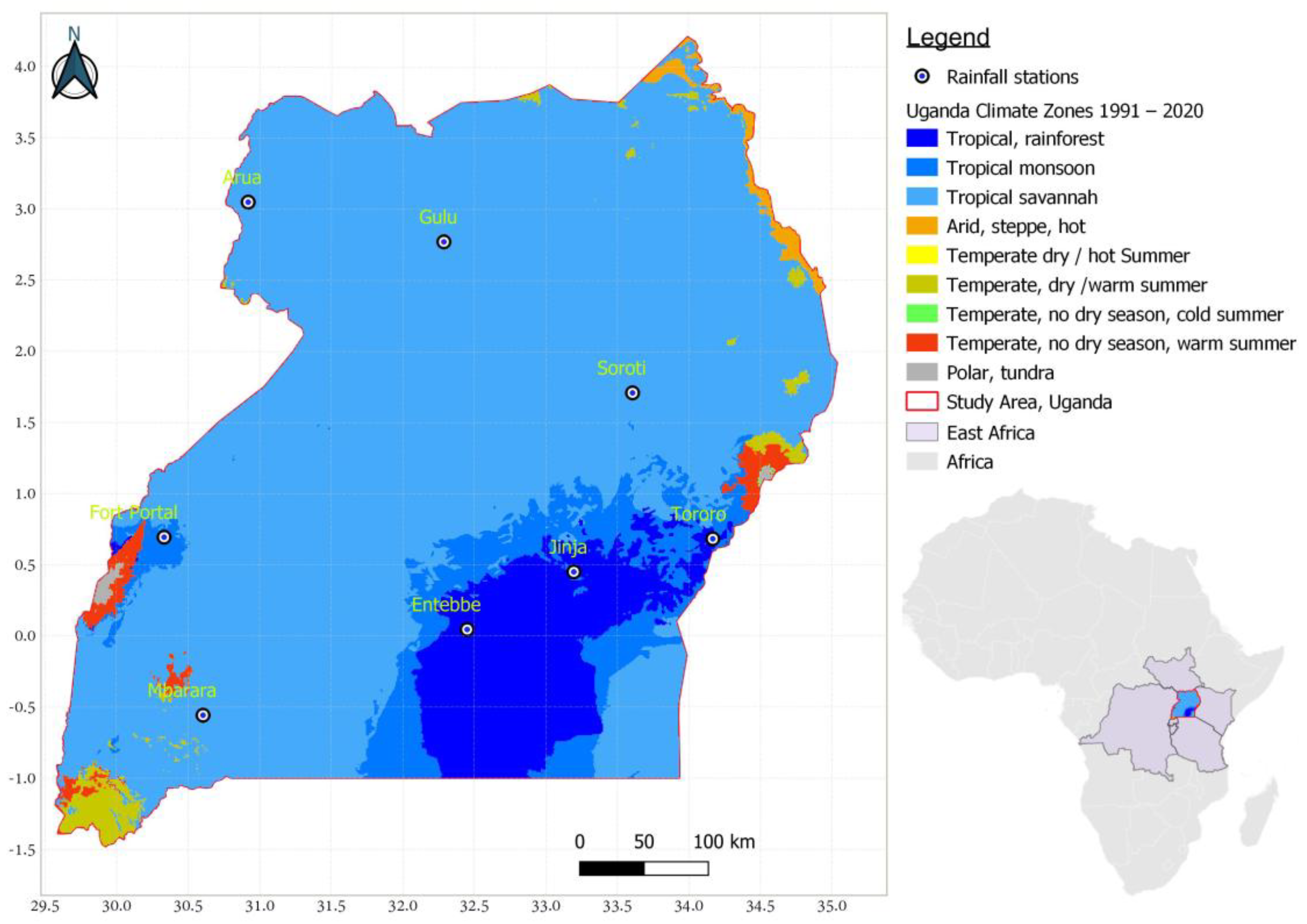
Figure 2.
Scatter plots of the actual and predicted coefficients considering the observed data.
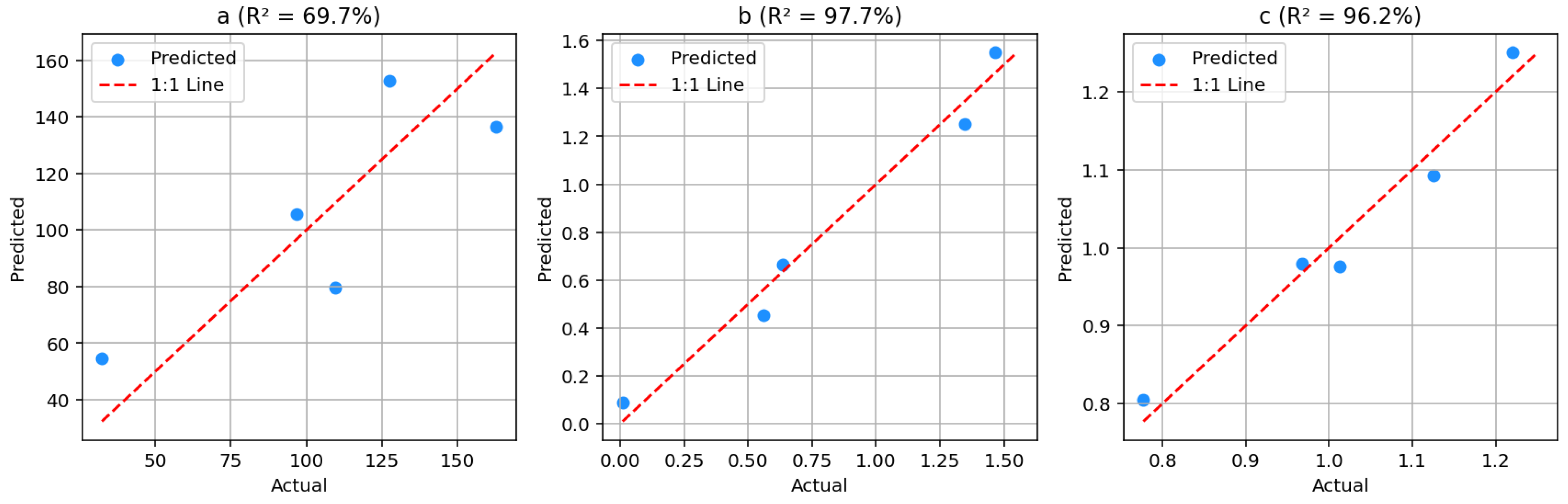
Figure 3.
Scatter plots of the actual and predicted coefficients considering disaggregated data.
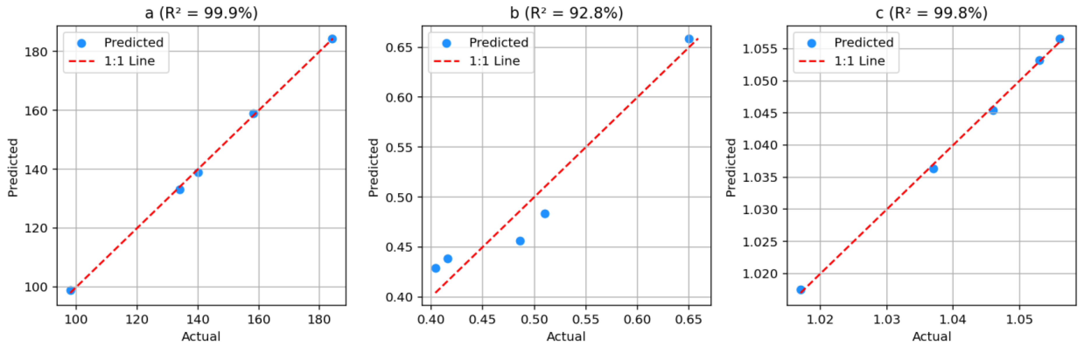
Table 1.
IDF coefficients from the aligned TD method and observed hourly rainfall data.
| S/No | Stations | From application of Aligned TD factors | Empirical (observed hourly rainfall data) | ||||||
|---|---|---|---|---|---|---|---|---|---|
| a | b | c | R2 | a | b | c | R2 | ||
| 1 | Gulu | 121.289 | 0.41 | 1.010 | 100 | 678.54 | 3.25 | 1.430 | 99.55 |
| 2 | Soroti | 158.25 | 0.416 | 1.017 | 100 | 32.37 | 0.01 | 0.777 | 97.15 |
| 3 | Jinja | 128.85 | 0.407 | 1.030 | 100 | 141.07 | 0.718 | 0.857 | 99.73 |
| 4 | Mbarara | 139.95 | 0.486 | 1.037 | 99.99 | 109.37 | 0.559 | 1.013 | 99.84 |
| 5 | Fort Portal | 97.97 | 0.404 | 1.056 | 99.99 | 127.53 | 1.464 | 1.220 | 99.33 |
| 6 | Arua | 134.080 | 0.510 | 1.046 | 99.99 | 162.842 | 1.346 | 1.125 | 99.88 |
| 7 | Entebbe | 184.107 | 0.650 | 1.053 | 100 | 96.758 | 0.634 | 0.968 | 99.95 |
| 8 | Tororo | 163.521 | 0.533 | 1.079 | 99.99 | 57.130 | 0.241 | 0.895 | 99.88 |
Table 2.
Elevations, means and standard deviations of the AMS rainfall data.
| Station | Longitude | Latitude | Elevation | Mean | s |
| Jinja | 33.19558 | 0.450418 | 1175 | 74.23 | 17.454 |
| Gulu | 32.2865 | 2.77233 | 1111 | 72.377 | 18.142 |
| Tororo | 34.167 | 0.683 | 1177 | 79.573 | 21.0222 |
| Mbarara | 30.60435 | -0.55794 | 1402 | 59.067 | 17.290 |
| Fort Portal | 30.33224 | 0.693556 | 1531 | 54.493 | 14.206 |
| Soroti | 33.6063 | 1.7098 | 1116 | 73.493 | 18.281 |
| Entebbe | 32.45 | 0.045 | 1150 | 87.573 | 25.299 |
| Arua | 30.917 | 3.05 | 1199 | 76.44 | 17.897 |
Table 3.
MRA model equations and performance based on observed rainfall data.
| Equations for each of the coefficients, a, b, and c | R2 (%) |
|---|---|
| 69.73 | |
| 97.65 | |
| 96.25 |
Table 4.
MRA model equations and performance based disaggregated rainfall data.
| Equations for each of the coefficients, a, b, and c | R2 (%) |
|---|---|
| 99.92 | |
| 92.81 | |
| 99.84 |
Table 5.
Comparison of actual (observed) and predicted coefficients via AE and PE.
| Station | Coefficient | Actual | Predicted | AE | PE |
| Jinja | a | 141.07 | 107.642 | 33.428 | -23.7 |
| Jinja | b | 0.718 | 0.856 | 0.138 | 19.2 |
| Jinja | c | 0.857 | 0.993 | 0.136 | 15.85 |
| Gulu | a | 678.54 | 42.687 | 635.853 | -93.71 |
| Gulu | b | 3.25 | -0.079 | 3.329 | -102.43 |
| Gulu | c | 1.43 | 0.765 | 0.665 | -46.53 |
| Tororo | a | 57.13 | 106.650 | 49.52 | 86.68 |
| Tororo | b | 0.241 | 0.767 | 0.526 | 218.44 |
| Tororo | c | 0.895 | 0.991 | 0.096 | 10.68 |
Table 6.
Comparison of actual (observed) and predicted coefficients via AE and PE.
| Station | Coefficient | Actual | Predicted | AE | PE |
| Jinja | a | 128.85 | 138.84 | 9.988 | 7.75 |
| Jinja | b | 0.41 | 0.45 | 0.046 | 11.22 |
| Jinja | c | 1.03 | 1.03 | 0.004 | 0.42 |
| Gulu | a | 121.29 | 161.50 | 40.208 | 33.15 |
| Gulu | b | 0.41 | 0.43 | 0.017 | 4.2 |
| Gulu | c | 1.01 | 1.01 | 0.003 | 0.32 |
| Tororo | a | 163.52 | 159.22 | 4.302 | -2.63 |
| Tororo | b | 0.53 | 0.55 | 0.015 | 2.78 |
| Tororo | c | 1.08 | 1.04 | 0.035 | -3.29 |
Disclaimer/Publisher’s Note: The statements, opinions and data contained in all publications are solely those of the individual author(s) and contributor(s) and not of MDPI and/or the editor(s). MDPI and/or the editor(s) disclaim responsibility for any injury to people or property resulting from any ideas, methods, instructions or products referred to in the content. |
© 2025 by the authors. Licensee MDPI, Basel, Switzerland. This article is an open access article distributed under the terms and conditions of the Creative Commons Attribution (CC BY) license (http://creativecommons.org/licenses/by/4.0/).
Copyright: This open access article is published under a Creative Commons CC BY 4.0 license, which permit the free download, distribution, and reuse, provided that the author and preprint are cited in any reuse.


