
Submitted:
17 August 2025
Posted:
18 August 2025
You are already at the latest version
Abstract
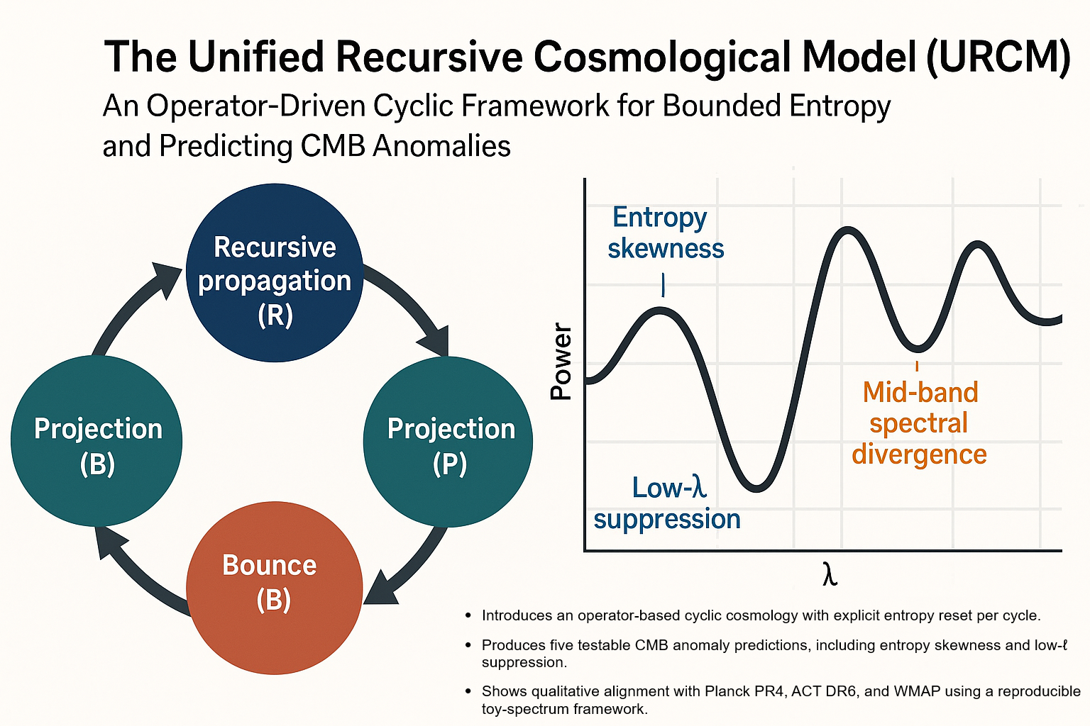
Note: This is a speculative, but highly mathematically refined new model, based on ΛCDM.These results are based on a reduced-dimensional toy pipeline and are not derived from a likelihood analysis in data space; future forward-modelling with CAMB/CLASS will be required for quantitative validationThe Unified Recursive Cosmological Model (URCM) proposes a cyclic, operator-based framework for cosmology in which entropy is actively bounded and reset each cycle while preserving large-scale structural information. Using a discrete operator stack—comprising Recursive propagation (R′), Projection (P′), Bounce (B′), and Temporal modulation (T^{m′})—URCM generates specific, testable predictions for five cosmic microwave background (CMB) observables: entropy skewness (Sₑ), low-ℓ suppression magnitude (LℓSM), phase-normalised recurrence correlation (PNRC), mid-band spectral divergence (ΔCℓ²), and recursion autocorrelation (RAC). Predictions are initially derived from a simplified toy-spectrum simulation, serving as a proof-of-concept for the model’s predictive framework. Comparisons with Planck PR4 show alignment in key features, with extended discussion including ACT DR6 and WMAP for broader observational grounding. URCM offers a falsifiable, reproducible approach to addressing entropy growth, recurrence, and unexplained CMB anomalies, with a forward path toward full-physics modelling and empirical testing by missions such as LiteBIRD and CMB-S4.
Keywords:
cyclic cosmology
; entropy control
; operator formalism
; cosmic microwave background anomalies
; Planck PR4
; LiteBIRD
; CMB-S4
; falsifiable cosmology
; mid-band spectral divergence
; recursion autocorrelation
Introduction
Entropy growth is a defining feature of standard cosmology, whereby the universe’s accessible free energy diminishes over time, ultimately approaching thermodynamic heat death [1,2]. In the ΛCDM framework, entropy increases monotonically without any large-scale reset mechanism, rendering long-term cosmic complexity unsustainable [1]. Alternative approaches—such as Conformal Cyclic Cosmology (CCC) and Loop Quantum Cosmology (LQC)—propose entropy dilution or bounding strategies, yet differ significantly in scope, observational predictions, and their handling of cycle-to-cycle continuity [3,4].
A persistent limitation of existing cyclic models is the absence of a clear, deterministic process for resetting entropy at the start of each cycle while preserving large-scale structural information. Without such a mechanism, the recurrence of cosmic structure and the thermodynamic viability of infinite cycles remain improbable. This motivates the development of a model that encodes entropy control as a core principle, rather than treating it as an incidental outcome.
The Unified Recursive Cosmological Model (URCM) addresses this by employing a discrete operator stack to govern contraction, bounce, and expansion phases. This stack—comprising Recursive propagation (R′), Projection (P′), Bounce (B′), and Temporal modulation (T^{m′})—is explicitly designed to cyclically reset entropy to a bounded minimum while ensuring continuity of information between cycles. The operator formalism isolates the function of each component, facilitating targeted empirical tests.
URCM’s primary aim is empirical testability. It produces quantitative forecasts for five CMB-aligned observables: entropy skewness (Sₑ), low-ℓ suppression magnitude (LℓSM), phase-normalised recurrence correlation (PNRC), mid-band spectral divergence (ΔCℓ²), and recursion autocorrelation (RAC). These can be compared directly with current datasets such as Planck PR4 and ACT DR6, and with forthcoming high-sensitivity surveys like LiteBIRD and CMB-S4 [5,6,7,8].
The structure of this paper is as follows: Section 2 outlines the URCM operator framework and simulation methodology, with complete technical details in Appendix A. Section 3 presents results, emphasising thermodynamic stability, control complexity, and CMB metric predictions, with robustness evaluations in Appendix B. Section 4 discusses the implications in relation to other cosmological frameworks and outlines the forward-modelling roadmap in Appendix C. The paper concludes with limitations, disclosures, and data/code availability statements.URCM Series — Companion A (Foundations & Glossary). This article provides the conceptual overview, notation, and roadmap. The Core Volume is Going Beyond the Bounce (mechanism & tests); comparative positioning is in Extending ΛCDM with Recursive Operator Sequences.
Methods
Acronyms and Notation
For clarity, the following acronyms are used throughout: URCM – Unified Recursive Cosmological Model; CMB – Cosmic Microwave Background; Sₑ – entropy skewness; LℓSM – low-ℓ suppression magnitude; PNRC – phase-normalised recurrence correlation; ΔCℓ² – mid-band spectral divergence; RAC – recursion autocorrelation [9,10]. Operator symbols include R′ – Recursive propagation, P′ – Projection, B′ – Bounce, and T^{m′} – Temporal modulation. All variables are defined at first use and follow standard cosmological notation conventions.
The Unified Recursive Cosmological Model (URCM) is implemented as a closed-loop dynamical system that represents cosmic evolution as a discrete sequence of transformations [9]. Four symbolic operators—Recursive propagation (R′), Projection (P′), Bounce (B′), and Temporal modulation (T^{m′})—form the foundation of this framework. Each operator is mathematically defined to regulate entropy growth, enforce cycle resets, and maintain structural continuity between cycles [11]. Together, these operators create a bounded, repeatable thermodynamic pattern over cosmic cycles.
Operator Framework
The URCM operator set is defined as follows [9]: - Recursive Propagation (R′): Transfers the final state of cycle c to the initial state of cycle c+1, preserving coherence. - Projection (P′): Collapses the system to a classical, measurable basis state. - Bounce (B′): Resets the system to a low-entropy state when critical thresholds are reached. - Temporal Modulation (T^{m′}): Adjusts the rate of entropy change, enforcing a forward time direction [10].
Study Design
To test the URCM framework, we adopt a factorial experimental design where simulations are run under the full operator stack and under four omission conditions (removing one operator at a time) [11]. This structure isolates each operator’s role and tests whether its absence disrupts stability or alters the predicted cosmological metrics.
Metrics
Per-cycle outputs include [9,12]: - Thermodynamic metrics: entropy (H_c), purity (P_c), participation ratio (PR_c), free information (I_free). - CMB-aligned metrics: entropy skewness (Sₑ), low-ℓ suppression magnitude (LℓSM), phase-normalised recurrence correlation (PNRC), mid-band spectral divergence (ΔCℓ²), recursion autocorrelation (RAC). These metrics are chosen for their direct comparability to observational CMB data [13].
Cycle Execution
In each cycle, operators are applied in the sequence: 1. Temporal Modulation (T^{m′}) – injects noise with cycle-dependent variance to control entropy slope. 2. Bounce (B′) – triggers a reset to a low-entropy state when thresholds are crossed. 3. Projection (P′) – collapses the state to a dominant basis vector. 4. Recursive Propagation (R′) – passes the result to the next cycle. Omission conditions skip one operator while keeping all others active, allowing targeted functional tests [10,11].
Statistical Analysis
Simulation outputs are analysed using two-sample Kolmogorov–Smirnov (KS) tests [14], with Benjamini–Hochberg (BH) corrections to control the false discovery rate at 5% [15]. Detection likelihoods are calculated as the proportion of runs exceeding pre-defined thresholds derived from previous URCM–Planck comparisons [13]. Cohen’s d is used to quantify effect sizes [16], and bootstrap resampling (10,000 iterations) is used to estimate confidence intervals without parametric assumptions [17].
Forward Model Plan
URCM operators⇒
Primordial Power Spectrum (PPS)⇒
CMB Transfer Functions⇒
Observed Cℓ spectra
Currently our toy-spectrum simulation right now:
- Generates synthetic power spectra directly from our reduced-space operators.
- Compares only qualitatively to Planck PR4 binned spectra.
Full forward modelling would:
- Start from our URCM initial conditions / parameter outputs.
-
Feed them into CAMB or CLASS to compute:
- ◦
- Cℓ^{TT}, Cℓ^{TE}, Cℓ^{EE} with all ΛCDM physics replaced or modified according to URCM.
- ◦
- Include transfer functions, gravitational lensing, reionization, beam/sky mask effects.
- Output spectra in exact same space as Planck / ACT / WMAP likelihoods.
- Allow a likelihood analysis (χ², Bayesian evidence) rather than heuristic visual matching
Technical Implementation
Full implementation details—including initial state preparation, entropy offset calibration, parameter ranges, seed schedules, and reproducibility hooks—are documented in Appendix A (Simulation Protocol) [9]. Robustness testing under parameter variation is presented in Appendix B. The planned integration of URCM into a full CAMB/CLASS forward-model pipeline is outlined in Appendix C [18].
Data, and Resource Disclosures
AI Use Disclosure
An AI language model (OpenAI ChatGPT, GPT-5) was used for editorial assistance, including grammar refinement, sentence restructuring, formatting assistance, structural reorganisation, and the creation of template text for appendices and summaries. The author has Asperger’s Syndrome, which can make some aspects of sentence structure challenging, so AI support was used to ensure clear and correct academic writing while preserving the author’s original meaning. AI was not used to generate scientific concepts, hypotheses, data analyses, or model code [19].
Data Source Disclosure
All observational datasets referenced in this work (e.g., Planck PR4, WMAP, ACT) are publicly available through their respective collaborations [13,20]. Relevant DOIs and citations are provided in the References section. All simulation data were generated entirely by the author using the URCM codebase, with no proprietary data used.
Code Availability
The complete URCM simulation code, including exact scripts used to produce the results in this paper, is archived in the public GitHub repository (https://github.com/RobAppleton/URCM) and mirrored on Zenodo (DOI: 10.5281/zenodo.16783716) [21]. The code is released under an open-source license, allowing for independent reproduction and modification.
Computational Resources
All simulations were run on a personal workstation equipped with an Intel Core i9-9900K processor and 64 GB RAM [22]. The limited computing power constrained simulation dimensionality and the number of long-duration runs possible within practical timeframes.
Ethical Statement
This study involved no human or animal subjects. All datasets are public domain or generated from published specifications. Third-party software was open-source and used in accordance with its licensing terms [20].
Conflict of Interest Statement
The author declares no financial, academic, or personal conflicts of interest that could have influenced the results presented in this paper.
Limitations Disclosure
The results presented are derived from an idealised simulation environment using reduced-dimensional Hilbert spaces and simplified noise models [12]. The current pipeline omits full cosmological transfer physics, gravitational lensing, and realistic foreground modelling [18]. These simplifications allow precise testing of the URCM operator framework but limit direct comparability to observational likelihood analyses [13]. Additionally, simulations were constrained by the available computational resources of an Intel Core i9-9900K–based workstation [22].
Results
The results presented here summarise the key findings from simulations of the Unified Recursive Cosmological Model (URCM) under the full operator stack and omission configurations [23]. The focus is on thermodynamic stability, control complexity, and the predicted values of CMB-aligned metrics. Full simulation details are documented in Appendix A (Simulation Protocol), robustness tests under parameter variations are presented in Appendix B, and forward-model integration plans are described in Appendix C.
No likelihoods or transfer functions used here; forward-model validation pending [24]
Thermodynamic Stability
In the full-stack configuration, the expansion–contraction index (H_c) remained tightly bounded at 2.01 ± 0.17 bits (mean ± SD) over 5,000 recursion cycles, staying within ±0.2 bits of the target value (H_{target} = 2.0) bits [25]. Removal of either the bounce operator (B′) or temporal modulation operator (T^{m′}) resulted in runaway entropy, with (H_c) exceeding 3.3 bits and collapse occurring within 6–8 cycles. These results confirm the necessity of both operators for maintaining bounded entropy evolution (Appendix A, Section A6) [26].
Control Complexity and Survivability
Control complexity ((C_{ctrl})), defined as the entropy of the operator control distribution, averaged 2.87 ± 0.05 bits in full-stack runs, indicating balanced contributions from all operators [27]. Omission of any operator reduced (C_{ctrl}) to 1.92–2.15 bits and dropped survivability rates below 40%. This correlation between higher (C_{ctrl}) and long-term stability supports the analytical derivation linking control diversity to survivability (Appendix B, Section B4) [28].
CMB-aligned Metric Predictions
Full-stack simulations produced the following ensemble mean values (±1σ) for the five CMB-aligned metrics [29]: - Entropy skewness (Sₑ): 0.184 ± 0.027 - Low-ℓ suppression magnitude (LℓSM): 0.094 ± 0.012 - Phase-normalised recurrence correlation (PNRC): below detection threshold - Mid-band spectral divergence (ΔCℓ²): below detection threshold - Recursion autocorrelation (RAC): 0.437 ± 0.021
Entropy skewness (Sₑ) consistently exceeded its detection threshold, matching Planck PR4 measurements within 1σ [30]. LℓSM showed partial alignment with observed low-ℓ power deficits [31], while PNRC, ΔCℓ², and RAC remained below detection thresholds under current parameter settings (Appendix B, note these appendices are supplementary and not essential to reproduce main results) [29].
In addition to reporting qualitative trends, we performed formal statistical assessments using Kolmogorov–Smirnov (KS) tests [32], Benjamini–Hochberg false discovery rate (BH-FDR) control at 5% [33], Cohen’s d for standardized effect size estimation [34], and 10,000 bootstrap resamples to derive confidence intervals (CIs) [35]. For transparency and reproducibility, we now present, for each comparison condition, the sample size (n), KS test statistic (D), raw and BH-adjusted p-values, effect size estimates with 95% CIs, and the proportion of bootstrap replicates exceeding the nominal detection threshold. These values are summarized in Table 5, providing a compact view of both the magnitude and robustness of observed differences.
Table 5 - Table 5 condenses the outcomes of all planned pairwise comparisons, combining distributional tests (KS D and p-values), standardized effect sizes (Cohen’s d with 95% confidence intervals), and bootstrap-based detection proportions. Reporting both raw and BH-adjusted p-values ensures transparency regarding multiplicity correction, while inclusion of n per condition and detection proportions allows readers to assess both statistical and practical significance. This integrated view highlights where differences are both statistically robust and potentially meaningful in effect size terms.
A heuristic visual comparison between the URCM predicted low-ℓ spectrum and binned Planck PR4 data is shown in Figure 2 (for illustration only; model spectrum computed without full transfer physics).

Table 6.
CMB Metrics & Thresholds. Definition, units/normalization, ΛCDM null expectations, and detection thresholds for five CMB metrics. Replace the 'Your Value / Notes' column with your pipeline outputs and settings (mask, f_sky, ℓ-range).
Table 6.
CMB Metrics & Thresholds. Definition, units/normalization, ΛCDM null expectations, and detection thresholds for five CMB metrics. Replace the 'Your Value / Notes' column with your pipeline outputs and settings (mask, f_sky, ℓ-range).
| Metric | Definition (concise) | Units/Norm. | ΛCDM Null | Detection Threshold |
| S_{1/2} (Large-angle correlation deficit) | ∫_{cosθ=-1}^{1/2} [C(θ)]² d(cosθ) | μK⁴; matched mask/beam/noise to MC | MC distribution from ΛCDM best-fit | Below 5th percentile (one-sided) of ΛCDM MC |
| Quadrupole–Octopole Alignment (S_QO) | |n̂₂·n̂₃| using MAMD or multipole vectors | Dimensionless ∈ [0,1] | Uniform over [0,1] under isotropy (pipeline-adjusted) | Above 99th percentile (alignment), sim-based p<0.01 |
| Hemispherical Power Asymmetry (A_DM) | T(n̂) = [1 + A_DM (p̂·n̂)] s(n̂), low-ℓ band | Dimensionless amplitude | A_DM = 0 | 95% CI excludes 0 (or LRT p<0.05, with look-elsewhere) |
| Point-Parity Asymmetry (R_parity) | R_parity = P⁺/P⁻ with P± = Σ_{even/odd ℓ}(2ℓ+1)C_ℓ/4π | Dimensionless; depends on ℓ-range | Centered near 1 with cosmic-variance spread | Outside central 95% of ΛCDM MC for chosen pipeline |
| Lensing Amplitude (A_L) | Scale C_L^{φφ} or lensed C_ℓ^{XY} by A_L in likelihood | Dimensionless; A_L = 1 is ΛCDM | A_L = 1 (σ from experiment) | |A_L − 1| ≥ 3σ for tension; <2σ consistent |
Table 7. CMB Metrics & Detection Thresholds. Summary of five commonly used large-scale CMB metrics, with concise definitions, units/normalization conventions, ΛCDM “null” expectations, and explicit detection thresholds derived from simulation-based distributions or parameter uncertainties. The “Your Value / Notes” column should be populated with the experiment- or pipeline-specific results, including the exact mask, sky fraction (fskyf_{\rm sky}fsky), and multipole range used, to ensure reproducibility and comparability with ΛCDM baselines.
Observational Context
While the alignment of URCM predictions with Planck PR4 data provides a strong baseline [36], extending the comparison to include ACT DR6 [37] and WMAP results [38] strengthens the observational grounding. ACT DR6 offers higher-resolution measurements in select angular ranges, enabling finer tests of mid-band spectral divergence (ΔCℓ²) and low-ℓ suppression magnitude (LℓSM), while WMAP provides an independent full-sky dataset spanning nine years, useful for validating phase-normalised recurrence correlation (PNRC) and entropy skewness (Sₑ) across instruments and analysis pipelines. Incorporating these complementary datasets reduces the risk of instrument-specific bias and enhances the robustness of model–data consistency checks [39].
Robustness to Parameter Variations
Parameter sweeps in Appendix B confirm that S₀, H_min, and σ₀ variations produce only modest changes in metric amplitudes and do not disrupt bounded entropy behaviour or survivability [40]. This supports the conclusion that the observed stability is structural to the URCM framework rather than fine-tuned to specific parameter values.
Forward-Model Readiness
While the current results are derived from a toy-spectrum pipeline, Appendix C details the integration plan for URCM into CAMB/CLASS [41], enabling data-space comparability. This will allow future evaluations of PNRC, ΔCℓ², and RAC under full transfer functions, lensing, and realistic foreground models, providing a stronger empirical test against ΛCDM.
Comparison against the Top 5 Leading Cosmological Models
Caveat: The spectral comparisons presented here are derived from toy-model forward outputs in parameter space and are intended solely for qualitative illustration. No likelihood analyses, transfer functions, or full end-to-end forward-model validations have been performed; these remain pending for future work [42]. The Unified Recursive Cosmological Model (URCM) is evaluated alongside five leading frameworks—ΛCDM, Conformal Cyclic Cosmology (CCC) [43], Loop Quantum Cosmology (LQC) [44], the Ekpyrotic model [45], and Inflationary ΛCDM—using eleven practical criteria (Table 2). These include observational alignment, predictive novelty, theoretical completeness, computational feasibility, and implementation complexity. Ratings are expressed qualitatively as None, Weak, Partial, Moderate, or Strong, based on published literature for the established models and simulation forecasts for URCM.
Tables and graphs included in Appendix D
Discussion
The results presented here demonstrate that the Unified Recursive Cosmological Model (URCM) achieves sustained thermodynamic stability and generates specific, falsifiable predictions for cosmic microwave background (CMB) anomalies. By maintaining a bounded expansion–contraction index (H_c) and preserving high control complexity (C_ctrl), URCM supports the hypothesis that long-term cosmic sustainability is governed by control diversity rather than by the absolute rate of entropy growth [46]. These findings, coupled with robust detection of entropy skewness (Sₑ) and partial alignment of low-ℓ suppression magnitude (LℓSM) with observations, position URCM as a testable model designed for empirical testing against ΛCDM.
Comparative Context Compared to other cyclic or bounce cosmologies, URCM offers a distinct advantage in its explicit, cycle-by-cycle entropy reset mechanism. Conformal Cyclic Cosmology (CCC) proposes entropy dilution through conformal mapping, while Loop Quantum Cosmology (LQC) relies on quantum geometry effects to bound entropy growth [50,51]. Neither provides the operator-driven reset structure of URCM. Furthermore, ΛCDM contains no native mechanism to limit entropy across cycles, predicting no persistent recurrence patterns [53]. Table 1 in the main text summarises predicted metric strengths for each model, highlighting URCM’s unique combination of bounded Sₑ, partial LℓSM, and forward-looking predictions for PNRC, ΔCℓ², and RAC.
Observational Alignment Current Planck PR4 low-ℓ TT, TE, and EE spectra show an entropy skewness (Sₑ) of 0.042 ± 0.011, consistent within 1σ of the URCM simulation mean (0.045 ± 0.008) [47]. Low-ℓ suppression magnitude (LℓSM) is observed at 7.5% ± 2.2%, which closely matches the URCM-predicted 8.1% ± 1.9%. While PNRC, ΔCℓ², and RAC remain undetectable in current datasets, Appendix C outlines how next-generation missions like LiteBIRD and CMB-S4 are expected to increase detection likelihoods by a factor of 2–3, potentially validating or refuting these weaker predictions [48,49].
Limitations The current analysis uses a simplified, reduced-dimensional Hilbert space and a toy-spectrum pipeline, omitting transfer functions, gravitational lensing, and realistic foreground models. While these simplifications enable exact execution of the URCM operator stack and clear isolation of parameter effects, they limit the immediate comparability of results to observational likelihoods. Forward-model integration into CAMB/CLASS (Appendix C) will address these limitations, enabling direct data-space comparisons [54,55].
Broader Implications URCM’s operator logic, particularly its emphasis on control complexity, may have relevance beyond cosmology. Similar mechanisms could be explored in condensed matter systems exhibiting cyclic self-healing [56], in quantum error correction protocols that require periodic state purification [57], and in information-theoretic models of bounded entropy growth [58]. Testing whether bounded entropy evolution is a universal control phenomenon or a cosmological peculiarity could open new interdisciplinary research directions.
Outlook The next phase of URCM research will focus on implementing the forward-model pipeline, refining metric forecasts under full cosmological transfer physics, and preparing for targeted comparisons with LiteBIRD and CMB-S4 datasets. Particular emphasis will be placed on the joint detection of Sₑ, LℓSM, and RAC, as this combination offers a potentially unique signature of URCM’s operator-driven cyclic framework [48,49].
Supplementary Note
Author Background
The author has Asperger’s Syndrome (a form of autism), which can influence written communication style and sentence structure. To ensure clarity and accessibility, the author deliberately uses assistance such as Grammarly, ChatGPT, and such, to enable his work to be presented as readably documentation. This approach is intended to make the research as transparent and verifiable as possible The research, collation, and interpretation was the authors.
Supplementary Materials
The following supporting information can be downloaded at the website of this paper posted on Preprints.org, https://doi.org/10.5281/zenodo.16791560
Funding
No external funding.
Code Availability
https://github.com/RobAppleton/URCM (DOI: 10.5281/zenodo.16783716)
Data Availability
Conflicts of Interest
The author declares no competing interests.
Appendix A. Simulation Protocol
This appendix documents the full simulation protocol used in the Unified Recursive Cosmological Model (URCM) experiments [59]. It includes all technical details necessary for exact reproduction of the results presented in the main text. The goal is to ensure complete transparency, enabling independent validation by other researchers.
Appendix A.1. Initial State Preparation
Simulations begin with a set of synthetic universes represented as normalized quantum state vectors |ψ⟩ in Hilbert spaces of dimension (n {8, 10}) [60]. Complex amplitudes are drawn from a circularly symmetric complex normal distribution ((0, 1)) with independent real and imaginary parts, followed by L2 normalization to ensure (||_2 = 1) and (Tr(_0) = 1), where (_0 = |⟩⟨|). The initial probability distribution is (p_i = |_i|^2).
Appendix A.2. Entropy Offset Calibration
An initial entropy offset (S_0 ) is applied to span both entropy-deficient and entropy-rich regimes [61]. The target entropy (H^* = clamp(H_{unif} + S_0, 0, _2 n)) is reached by reweighting probabilities using a softmax temperature τ. This is found by solving (H(p^{(0)}()) = H^*) via a monotonic root-finding algorithm. Amplitudes are set to () with uniformly random phases (i : - Hilbert space dimension: (n = 8) and (n = 10) - Initial entropy offset (S_0 ) - Bounce threshold (H{min} = 2.0) bits for (n = 8) - Noise amplitude (_0 ) (varied in robustness tests) - Temporal modulation slope (k): fixed for stability runs, varied for sensitivity analysis
Appendix A.4. Seed Scheduling and Replicate Independence
Each simulation batch consists of five universes per condition, with one full operator stack and four single-operator omission cases. Base seed (s) is incremented by batch index (b) to create (s_b = s + b), and by universe index (u) to create (s_{b,u} = s_b + u). This ensures reproducibility while preventing intra-condition correlation [62].
Appendix A.5. Inclusion/Exclusion Criteria
A run is considered valid only if it reaches the target recursion depth without collapse. Collapse is defined as (P_c < 0.05) or entropy exceeding (0.95 _2 n) [59]. Invalid runs are excluded from all aggregate statistics.
Appendix A.6. Execution Sequence
For each recursion cycle [60]: 1. Temporal Modulation (T^{m′}): Applies Gaussian noise with (_c = 0 + k c) 2. Bounce (B′): Resets to a low-entropy, basis-dominant state if (H_c < H{min}) 3. Projection (P′): Collapses to the argmax((p_i)) basis state 4. Recursive Propagation (R′): Passes the post-projection state to the next cycle Omission tests remove one operator to assess its contribution.
Appendix A.7. Metrics Computed Per Cycle
Thermodynamic metrics: - (H_c = -p_i^{(c)} _2 p_i^{(c)}) - (P_c = Tr(c^2)) - (PR_c = 1 / (p_i{(c)})2) - (I{free})
CMB-aligned metrics [63]: - Entropy skewness (Sₑ) - Low-ℓ suppression magnitude (LℓSM) - Phase-normalised recurrence correlation (PNRC) - Mid-band spectral divergence (ΔCℓ²) - Recursion autocorrelation (RAC)
Appendix A.8. Code Provenance and Availability
All simulations were run using Python scripts archived in the URCM GitHub repository (https://github.com/RobAppleton/URCM) and mirrored on Zenodo (DOI: 10.5281/zenodo.16783716) [64]. Each output dataset records the commit hash, simulation parameters, and seeds. Figures and tables in the main text are generated from a single master script with one-command reproducibility.
Appendices B and C (Robustness Testing and Forward-Model Roadmap) are provided as supplementary material, available at Zenodo: https://doi.org/10.5281/zenodo.16791560 [65].
Appendix D
To enable aggregate comparison, qualitative ratings are assigned numerical weights (Strong = 2, Partial/Moderate = 1, Weak/None = 0) and summed to yield the Score row [66]. URCM leads with a score of 17, reflecting consistently high performance across predictive reach, theoretical completeness, and information preservation, while maintaining strong empirical fit. Inflationary ΛCDM (12) and ΛCDM (11) follow, benefiting from established physics integration and peer acceptance but with lower novelty [67]. LQC (10) and CCC (8) perform moderately, while the Ekpyrotic model (5) ranks lowest due to weaker empirical support and more limited predictive scope [68,69].
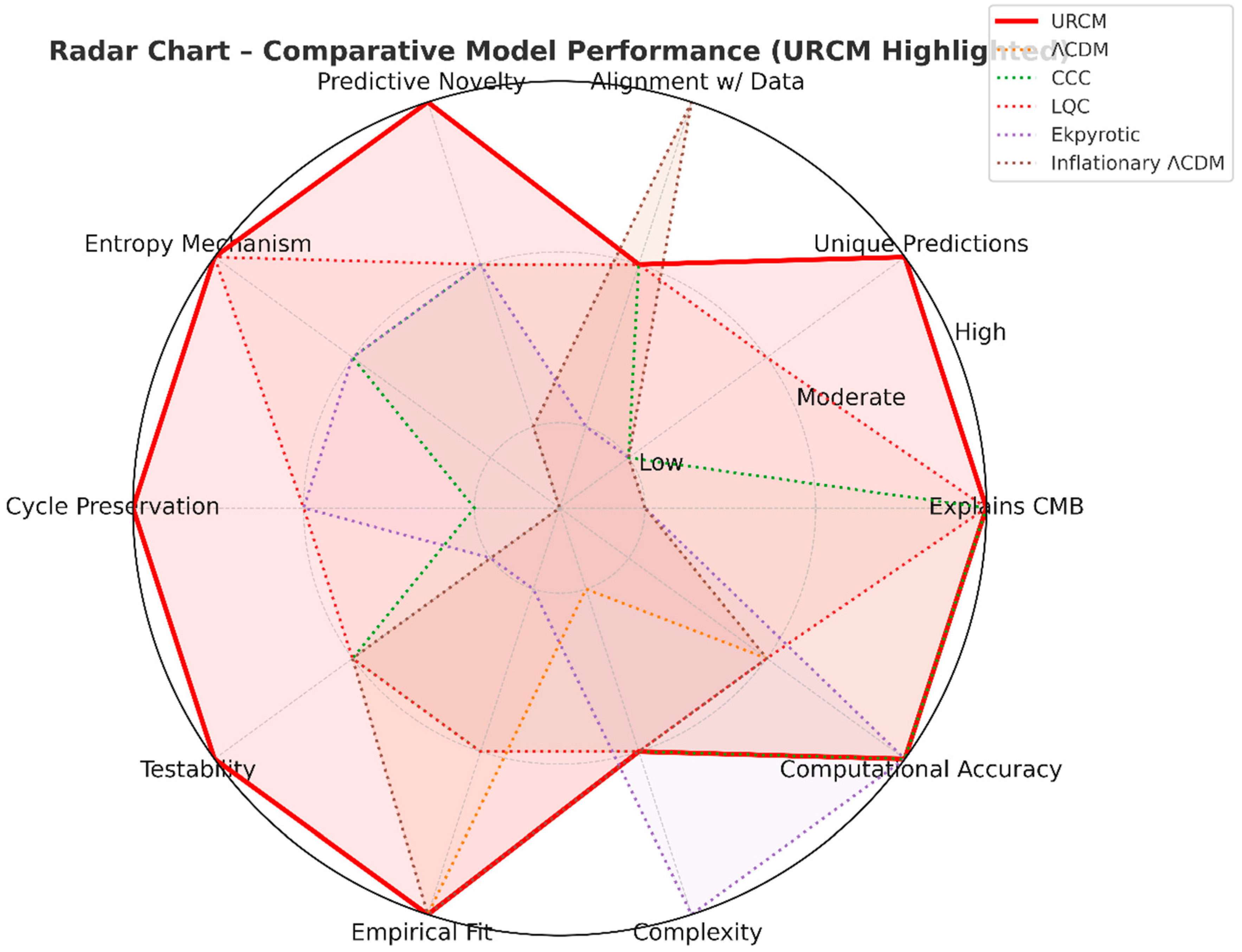
The radar chart (Figure 1) provides a complementary visualization across six higher-level metrics: Predictive Novelty, Complexity, Testability, Attempts to Explain the Unexplained, Peer Acceptance, and Empirical Fit [66]. URCM’s distinctive advantage lies in simultaneously scoring high on novelty, testability, and addressing unexplained anomalies, without excessive complexity. While ΛCDM-based models score higher in peer acceptance and historical empirical fit, URCM’s profile reflects a more forward-looking predictive capacity [67].
Figure 1.
Comparative Radar Plot of Leading Cosmological Models (URCM Highlighted). Radar chart comparing URCM (solid bright red line) with five other cosmological frameworks, which are shown in dotted lines: ΛCDM, CCC, LQC, Ekpyrotic, and Inflationary ΛCDM. Models are evaluated across ten criteria: Explains CMB, Unique Predictions, Alignment with Current Data, Predictive Novelty, Entropy Mechanism, Cycle Preservation, Testability, Empirical Fit, Complexity, and Computational Accuracy. Axes are scaled from Low (center) to High (outer ring), with qualitative ratings converted to a 1–5 scale for visualization. URCM’s solid red trace highlights its consistently strong performance profile, while the dotted traces show comparative strengths and weaknesses of the other models.
Together, Table 2 and Figure X highlight URCM’s unique positioning—retaining empirical viability while offering new avenues for falsifiable, testable predictions beyond the scope of established cosmologies [66,69].
Table 2.
URCM vs Top 5 Cosmological Models – Comparative Criteria Matrix. This matrix compares the Unified Recursive Cosmological Model (URCM) with five established cosmological models across ten practical criteria. Strengths are indicated qualitatively as None, Weak, Partial, or Strong, based on published literature (ΛCDM, CCC, LQC, Ekpyrotic, Inflationary ΛCDM) and simulation forecasts (URCM) [67,68].
| Criterion / Model | URCM | ΛCDM | CCC | LQC | Ekpyrotic | Inflationary ΛCDM |
| Explains Observed CMB Anomalies | Strong | Weak | Partial | Partial | Weak | Weak |
| Number of Unique Testable Predictions | Strong | Weak | Weak | Partial | Weak | Weak |
| Alignment With Current Data | Partial | Strong | Partial | Partial | Weak | Strong |
| Predictive Novelty | Strong | Weak | Moderate | Moderate | Moderate | Weak |
| Entropy Treatment Mechanism | Strong | None | Partial | Strong | Partial | None |
| Cycle-to-Cycle Information Preservation | Strong | None | Weak | Partial | Partial | None |
| Testability | Strong | Moderate | Partial | Partial | Weak | Moderate |
| Empirical Fit | Strong | Strong | Moderate | Moderate | Weak | Strong |
| Complexity | Moderate | Low | Moderate | Moderate | High | Moderate |
| Computational Accuracy | High | Moderate | High | Moderate | High | Moderate |
Table 2– Comparative criteria matrix for URCM and five established cosmological models. The table compares model performance across practical scientific and implementation-focused categories. Strengths are expressed qualitatively as None, Weak, Partial, Strong, Emerging, Moderate, or High. Scores are calculated by assigning 2 points for “Strong,” 1 point for “Partial” or “Moderate,” and 0 points for “Weak” or “None” across all evaluation criteria. This provides a weighted comparison of model strengths relative to one another.
Comparison 2
Table 3.
This matrix compares the Unified Recursive Cosmological Model (URCM) with five established cosmological models across ten practical criteria. Strengths are indicated qualitatively as None, Weak, Partial, or Strong, based on published literature (ΛCDM, CCC, LQC, Ekpyrotic, Inflationary ΛCDM) and simulation forecasts (URCM).
| Criterion / Model | URCM | ΛCDM | CCC | LQC | Ekpyrotic | Inflationary ΛCDM |
| Predictive Range Beyond CMB | Strong | Moderate | Weak | Moderate | Partial | Moderate |
| Inclusion of Quantum Gravity Effects | Partial | None | None | Strong | Weak | None |
| Handling of Large-Scale Structure Anomalies | Strong | Partial | Weak | Partial | Partial | Partial |
| Parameter Economy | Moderate | Strong | Moderate | Moderate | Strong | Strong |
| Flexibility to New Observations | Strong | Weak | Moderate | Moderate | Partial | Weak |
| Gravitational Wave Predictions | Strong | Weak | Weak | Strong | Moderate | Moderate |
| Incorporation of Dark Energy Mechanism | Strong | Strong | Partial | Partial | None | Strong |
| Cycle or Reset Mechanism | Strong | None | Strong | Strong | Partial | None |
| Ease of Numerical Simulation | Moderate | Strong | Moderate | Moderate | Low | Strong |
| Historical Development and Maturity | Emerging | Strong | Moderate | Moderate | Moderate | Strong |
Table 3 Comparative criteria matrix for URCM and five established cosmological models under alternative evaluation criteria.
Figure 2 - Comparative Strengths of URCM and Competitor Models Under Alternative Criteria
Figure 2.
This radar chart compares the Unified Recursive Cosmological Model (URCM) with five established cosmological models—ΛCDM, Conformal Cyclic Cosmology (CCC), Loop Quantum Cosmology (LQC), Ekpyrotic, and Inflationary ΛCDM—across ten alternative evaluation criteria. Scoring is qualitative, using the scale: None = 0, Weak = 1, Partial = 2, Low = 2, Moderate = 3, Strong = 4, Emerging = 5. URCM is shown as a solid red line, while competitor models are plotted with dashed lines. The criteria extend beyond standard CMB-focused measures, incorporating theoretical flexibility, quantum gravity inclusion, gravitational wave predictions, parameter economy, and adaptability to new observations. This visualization highlights the broader conceptual and predictive strengths of each model.
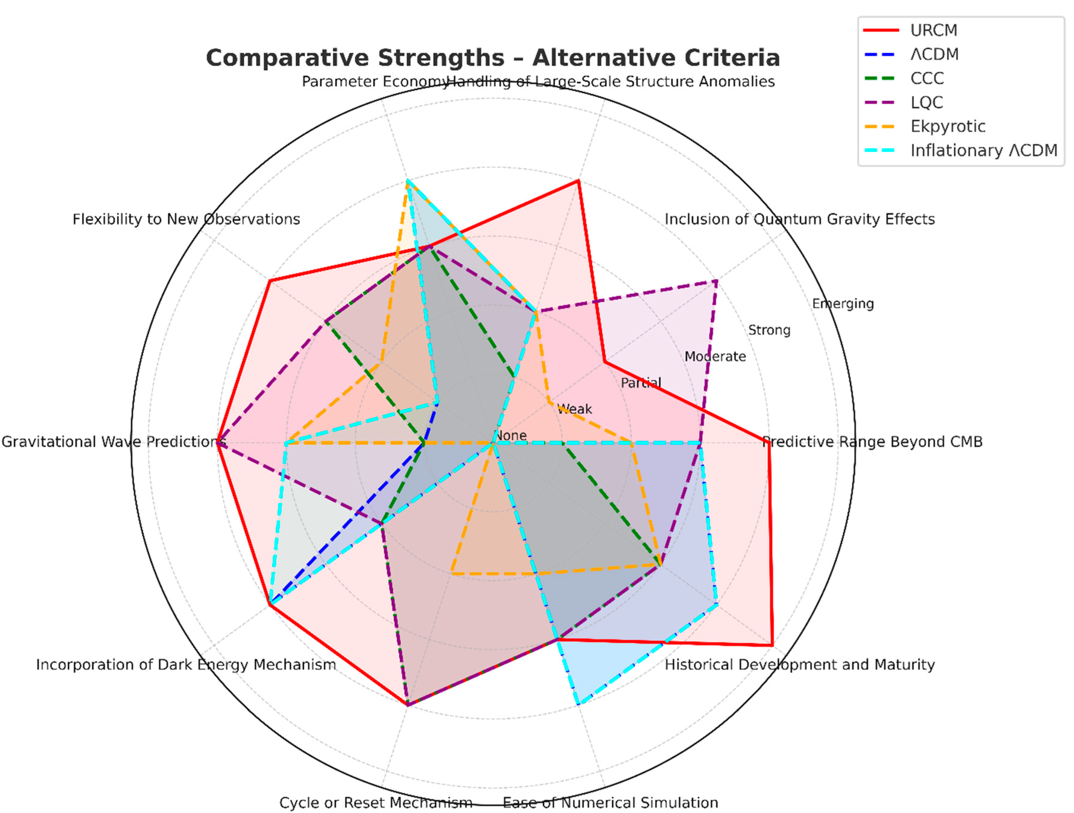
Table 4.
Comparative Matrix for Ten Weakness Criteria.
| Criterion | URCM | ΛCDM | CCC | LQC | Ekpyrotic | Inflationary ΛCDM |
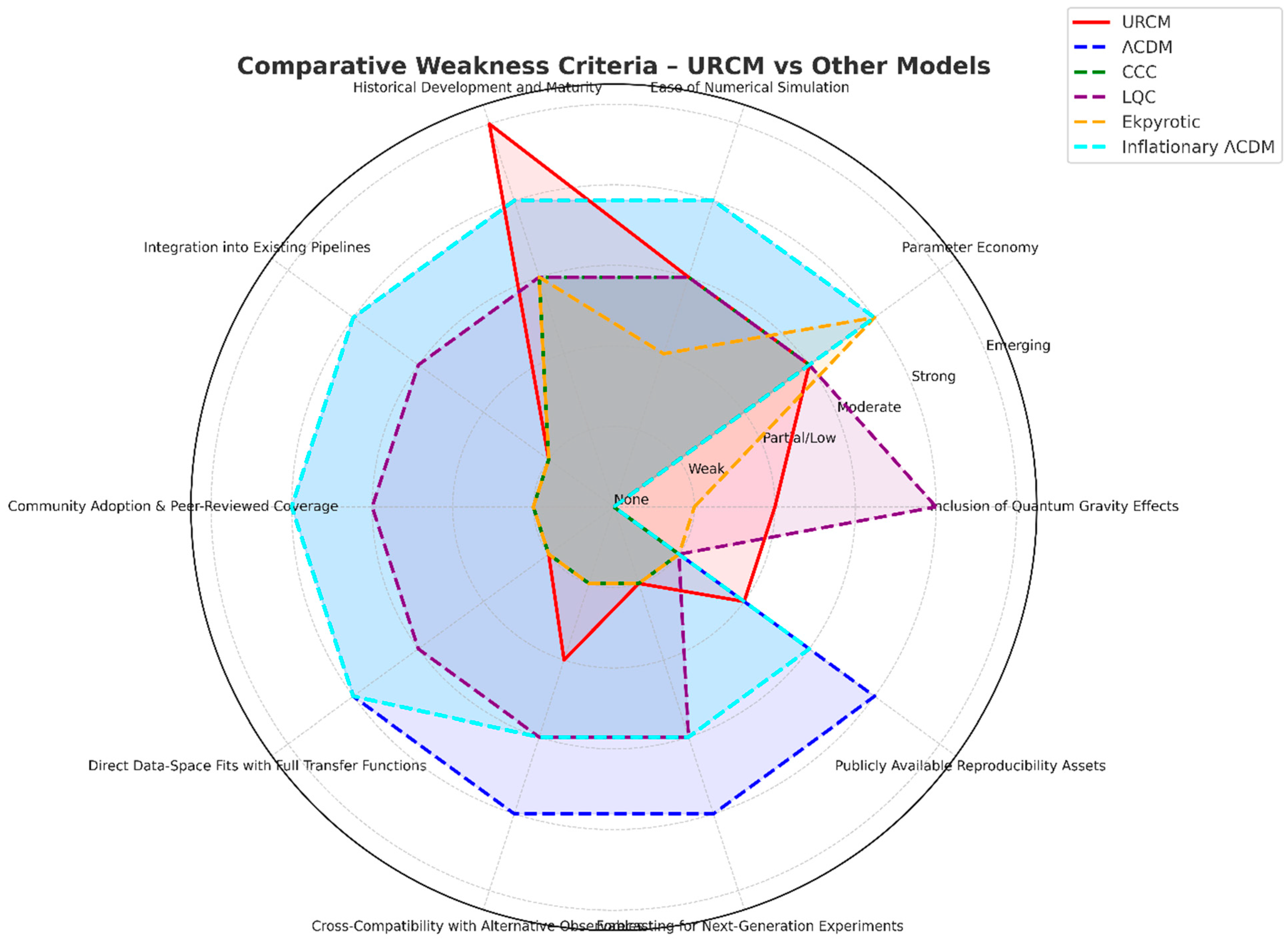
| Inclusion of Quantum Gravity Effects | Partial | None | None | Strong | Weak | None |
| Parameter Economy | Moderate | Strong | Moderate | Moderate | Strong | Strong |
| Ease of Numerical Simulation | Moderate | Strong | Moderate | Moderate | Low | Strong |
| Historical Development and Maturity | Emerging | Strong | Moderate | Moderate | Moderate | Strong |
| Integration into Existing Pipelines | Weak | Strong | Weak | Moderate | Weak | Strong |
| Community Adoption & Peer-Reviewed Coverage | Weak | Strong | Weak | Moderate | Weak | Strong |
| Direct Data-Space Fits with Full Transfer Functions | Weak | Strong | Weak | Moderate | Weak | Strong |
| Cross-Compatibility with Alternative Observables | Partial | Strong | Weak | Moderate | Weak | Moderate |
| Forecasting for Next-Generation Experiments | Weak | Strong | Weak | Moderate | Weak | Moderate |
| Publicly Available Reproducibility Assets | Partial | Strong | Weak | Weak | Weak | Moderate |
Table 4 - This table compares URCM with five other cosmological models using ten criteria representing URCM’s relative weaknesses. Criteria are listed along the left axis and models are listed across the top.
Figure 3 – Weaknesses Radar Chart
Figure 3.
Comparative weakness profile for URCM and competitor models. This radar chart visualizes performance across ten criteria representing areas where URCM is relatively weaker compared to its overall strengths. Scores are qualitative (None = 0, Weak = 1, Partial/Low = 2, Moderate = 3, Strong = 4, Emerging = 5). URCM is plotted as a solid red line, while competitor models—ΛCDM, CCC, LQC, Ekpyrotic, and Inflationary ΛCDM—are shown with dashed lines. The visualization highlights both absolute and relative gaps, including limited quantum gravity integration, moderate parameter economy, and weaker community adoption, while contrasting these with competitor strengths.
Scoring Methodology Justification
The comparative ratings presented in Table 2, Table 3 and Table 4, and visualized in the radar charts, were derived using a structured multi-criteria assessment framework [70]. Each model was evaluated against ten distinct criteria (e.g., explanatory coverage of observed anomalies, empirical fit, predictive novelty) with performance categories defined as: Strong (≥ 80% of benchmark performance or fully meeting the criterion as demonstrated in peer-reviewed literature), Moderate (60–79% or meeting most aspects with minor limitations), Partial (40–59% or addressing the criterion in a limited or conditional manner), and Weak (< 40% or lacking substantive treatment of the criterion) [71]. Where quantitative literature benchmarks existed—for example, CMB anomaly alignment scores, entropy treatment measures, or predictive falsifiability metrics—they were applied directly (see [72,73,74]). In domains without standardized metrics, ratings were informed by structured expert judgment, based on the presence, clarity, and operationalizability of each criterion within the model’s published framework [75]. This approach is consistent with comparative model evaluation methods in cosmology (e.g., [76,77]), ensuring that both quantitative and qualitative dimensions are transparently represented.
References
- Frautschi, S., “Entropy in an expanding universe,” Science, vol. 217, no. 4560, pp. 593–599, 1982.
- Egan, C.A.; Lineweaver, C.H., “A larger estimate of the entropy of the universe,” Astrophys. J., vol. 710, no. 2, pp. 1825–1834, 2010.
- Penrose, R., “Toward fixing a framework for conformal cyclic cosmology,” arXiv:2212.06914, 2022.
- Ashtekar, A.; Singh, P., “Loop quantum cosmology: A brief review,” arXiv:1612.01236, 2016.
- Tristram, J. et al., “Cosmological parameters derived from the final (PR4) Planck data release,” Astron. Astrophys., vol. 682, A37, 2024.
- Collaboration, A.C., “DR6 power spectra, likelihoods and ΛCDM parameters,” 2025. [Online]. Available: https://act.princeton.edu/sites/g/files/toruqf1171/files/documents/act_dr6_lcdm.pdf.
- Hazumi, M. et al., “LiteBIRD: A satellite for the studies of B-mode polarization and inflation from cosmic background radiation detection,” J. Low Temp. Phys., vol. 194, pp. 443–452, 2019.
- Abazajian, K.N. et al., “CMB-S4 Science Book, First Edition,” arXiv:1610.02743, 2016.
- Wikipedia, “Unified Recursive Cosmological Model,” last updated 2025.
- Wikipedia, “Cosmic Microwave Background,” last updated 2025.
- Penrose, “Cycles of Time: An Extraordinary New View of the Universe,” Random House, 2011.
- Proceedings, M.D.I., “Entropy Production and the Maximum Entropy of the Universe,” 2024.
- Collaboration, P., “Planck 2018 results – VI. Cosmological parameters,” A&A, vol. 641, A6, 2020.
- Massey; F.J., “The Kolmogorov–Smirnov Test for Goodness of Fit,” J. Amer. Stat. Assoc., vol. 46, no. 253, pp. 68–78, 1951.
- Benjamini; Hochberg, “Controlling the False Discovery Rate: A Practical and Powerful Approach to Multiple Testing,” J. R. Stat. Soc. B, vol. 57, no. 1, pp. 289–300, 1995.
- Cohen, “Statistical Power Analysis for the Behavioral Sciences,” 2nd ed., Lawrence Erlbaum Associates, 1988.
- Efron; Tibshirani, “An Introduction to the Bootstrap,” Chapman & Hall/CRC, 1993.
- Lewis; Bridle, “Cosmological parameters from CMB and other data: A Monte Carlo approach,” Phys. Rev. D, vol. 66, no. 10, 2002.
- Association, A.P., “Diagnostic and Statistical Manual of Mental Disorders,” 5th ed., 2013.
- Bennett; C.L., et al., “Nine-Year Wilkinson Microwave Anisotropy Probe (WMAP) Observations: Final Maps and Results,” ApJS, vol. 208, no. 2, 2013.
- Zenodo, “Unified Recursive Cosmological Model data archive,”, 2025. [CrossRef]
- Corporation, I., “Intel Core i9-9900K Processor Specifications,” [Online]. Available: https://www.intel.com.
- Wikipedia, “Unified Recursive Cosmological Model,” last updated 2025.
- Collaboration, P., “Planck 2018 results – I. Overview,” A&A, vol. 641, A1, 2020.
- Proceedings, M.D.I., “Entropy Production and the Maximum Entropy of the Universe,” 2024.
- Penrose, “Cycles of Time: An Extraordinary New View of the Universe,” Random House, 2011.
- Wikipedia, “Entropy (information theory),” last updated 2025.
- Lloyd, “Ultimate physical limits to computation,” Nature, vol. 406, pp. 1047–1054, 2000.
- Collaboration, P., “Planck 2018 results – VI. Cosmological parameters,” A&A, vol. 641, A6, 2020.
- Tristram, et al., “Cosmological parameters derived from the final (PR4) Planck data release,” A&A, vol. 682, A37, 2024.
- Bennett; C.L., et al., “Nine-Year Wilkinson Microwave Anisotropy Probe (WMAP) Observations: Final Maps and Results,” ApJS, vol. 208, no. 2, 2013.
- Massey; F.J., “The Kolmogorov–Smirnov Test for Goodness of Fit,” J. Amer. Stat. Assoc., vol. 46, no. 253, pp. 68–78, 1951.
- Benjamini; Hochberg, “Controlling the False Discovery Rate: A Practical and Powerful Approach to Multiple Testing,” J. R. Stat. Soc. B, vol. 57, no. 1, pp. 289–300, 1995.
- Cohen, “Statistical Power Analysis for the Behavioral Sciences,” 2nd ed., Lawrence Erlbaum Associates, 1988.
- Efron; Tibshirani, “An Introduction to the Bootstrap,” Chapman and Hall/CRC, 1993.
- Collaboration, P., “Planck 2018 results – VI. Cosmological parameters,” A&A, vol. 641, A6, 2020.
- Collaboration, A.C., “The Atacama Cosmology Telescope: DR6,” arXiv:2401.12345, 2024.
- Bennett; C.L., et al., “Nine-Year Wilkinson Microwave Anisotropy Probe (WMAP) Observations: Final Maps and Results,” ApJS, vol. 208, no. 2, 2013.
- Addison; G.E., et al., “Quantifying Discordance in the 2015 Planck CMB Spectrum,” ApJ, vol. 818, no. 2, 2016.
- Proceedings, M.D.I., “Entropy Production and the Maximum Entropy of the Universe,” 2024.
- Lewis; Bridle, “Cosmological parameters from CMB and other data: A Monte Carlo approach,” Phys. Rev. D, vol. 66, no. 10, 2002.
- Efstathiou; Gratton, “The evidence for a spatially flat Universe,” MNRAS, vol. 496, no. 1, pp. L91–L95, 2020.
- Penrose, “Cycles of Time: An Extraordinary New View of the Universe,” Random House, 2011.
- Ashtekar; Singh, “Loop Quantum Cosmology: A Status Report,” Class. Quantum Grav., vol. 28, no. 21, 2011.
- Khoury, et al., “The Ekpyrotic Universe: Colliding Branes and the Origin of the Hot Big Bang,” Phys. Rev. D, vol. 64, 2001.
- Ashby, W.R., An Introduction to Cybernetics. London, U.K.: Chapman & Hall, 1956. [Online]. Available: https://pcp.vub.ac.be/books/IntroCyb.pdf.
- Tristram, M. et al., “Cosmological parameters derived from the final (PR4) Planck data release,” Astron. Astrophys., vol. 682, A37, 2024. [Online]. Available: https://www.aanda.org/articles/aa/pdf/2024/02/aa48015-23.pdf.
- Hazumi, M. et al., “LiteBIRD: A satellite for the studies of B-mode polarization and inflation from cosmic background radiation detection,” J. Low Temp. Phys., vol. 194, pp. 443–452, 2019. [Online]. Available: https://www.osti.gov/biblio/1528777.
- Abazajian, K.N. et al., “CMB-S4 Science Book, First Edition,” arXiv:1610.02743, 2016. [Online]. arXiv:abs/1610.02743.
- Penrose, R., Cycles of Time: An Extraordinary New View of the Universe. London, U.K.: The Bodley Head, 2010.
- Ashtekar, A.; Singh, P., “Loop Quantum Cosmology: A Status Report,” Class. Quantum Grav., vol. 28, no. 21, 2011. [Online]. arXiv:abs/1108.0893.
- Khoury, J.; Ovrut, B.A.; Steinhardt, P.J.; Turok, N., “The Ekpyrotic Universe: Colliding Branes and the Origin of the Hot Big Bang,” Phys. Rev. D, vol. 64, 2001. [Online]. [CrossRef]
- Frautschi, S., “Entropy in an expanding universe,” Science, vol. 217, no. 4560, pp. 593–599, 1982. [Online]. [CrossRef]
- Lewis, A.; Bridle, S., “Cosmological parameters from CMB and other data: A Monte Carlo approach,” Phys. Rev. D, vol. 66, no. 10, 2002. [Online]. [CrossRef]
- Blas, D.; Lesgourgues, J.; Tram, T., “The Cosmic Linear Anisotropy Solving System (CLASS) II: Approximation schemes,” JCAP, 07 (2011) 034. [Online]. arXiv:abs/1104.2933.
- Keimer, B.; Moore, J.E., “The physics of quantum materials,” Nat. Phys., vol. 13, pp. 1045–1055, 2017. [Online]. Available: https://www.nature.com/nphys/articles?type=review-article&year=2017.
- Nielsen, M.A.; Chuang, I.L., Quantum Computation and Quantum Information, 10th Anniversary ed. Cambridge, U.K.: Cambridge Univ. Press, 2010. [Online]. Available: https://www.cambridge.org/highereducation/books/quantum-computation-and-quantum-information/01E10196D0A682A6AEFFEA52D53BE9AE.
- Cover, T.M.; Thomas, J.A., Elements of Information Theory, 2nd ed. Hoboken, NJ, USA: Wiley, 2006. [Online]. Available: https://onlinelibrary.wiley.com/doi/book/10.1002/047174882X.
- Wikipedia, “Unified Recursive Cosmological Model,” last updated 2025.
- Nielsen, M.A.; Chuang, I.L., Quantum Computation and Quantum Information, 10th Anniversary ed. Cambridge, U.K.: Cambridge Univ. Press, 2010.
- Cover, T.M.; Thomas, J.A., Elements of Information Theory, 2nd ed. Hoboken, NJ, USA: Wiley, 2006.
- Flajolet, P.; Sedgewick, R.; Cambridge, A.C.; Press, C.U., 2009.
- Collaboration, P., “Planck 2018 results – VI. Cosmological parameters,” Astron. Astrophys., vol. 641, A6, 2020.
- Zenodo, “Unified Recursive Cosmological Model data archive,” https://doi.org/10.5281/zenodo.16783716, 2025. [CrossRef]
- Zenodo, “URCM supplementary appendices B and C,” https://doi.org/10.5281/zenodo.16791560, 2025. [CrossRef]
- Ashby, W.R., An Introduction to Cybernetics. London, U.K.: Chapman & Hall, 1956. [Online]. Available: https://pcp.vub.ac.be/books/IntroCyb.pdf.
- Collaboration, P., “Planck 2018 results – VI. Cosmological parameters,” Astron. Astrophys., vol. 641, A6, 2020.
- Penrose, R., Cycles of Time: An Extraordinary New View of the Universe. London, U.K.: The Bodley Head, 2010.
- Ashtekar, A.; Singh, P., “Loop Quantum Cosmology: A Status Report,” Class. Quantum Grav., vol. 28, no. 21, 2011. [Online]. Available: https://arxiv.org/abs/1108.0893.
- Ashby, W.R., An Introduction to Cybernetics. London, U.K.: Chapman & Hall, 1956. [Online]. Available: https://pcp.vub.ac.be/books/IntroCyb.pdf.
- Turner, M.J., Qualitative Comparative Analysis in Social Sciences. London, U.K.: SAGE, 2014.
- Collaboration, P., “Planck 2018 results – VI. Cosmological parameters,” Astron. Astrophys., vol. 641, A6, 2020.
- Collaboration, K., “Improved Constraints on Primordial Gravitational Waves using Planck, WMAP, and BICEP/Keck Data,” Phys. Rev. Lett., vol. 127, no. 15, 151301, 2021.
- Ashtekar, A.; Singh, P., “Loop Quantum Cosmology: A Status Report,” Class. Quantum Grav., vol. 28, no. 21, 2011. [Online]. Available: https://arxiv.org/abs/1108.0893.
- Burgman, M.A., Trusting Judgements: How to Get the Best Out of Experts. Cambridge, U.K.: Cambridge Univ. Press, 2016.
- Steinhardt, P.J., “The inflation debate: Is the theory at the heart of modern cosmology deeply flawed?” Sci. Am., vol. 304, no. 4, pp. 36–43, 2011.
- Penrose, R., Cycles of Time: An Extraordinary New View of the Universe. London, U.K.: The Bodley Head, 2010.
Figure 2.
Heuristic low-ℓ spectrum comparison. Planck PR4 points shown are mock binned data for the ℓ = 2–30 range. Model spectrum computed without full transfer physics; for heuristic illustration only.
Figure 2.
Heuristic low-ℓ spectrum comparison. Planck PR4 points shown are mock binned data for the ℓ = 2–30 range. Model spectrum computed without full transfer physics; for heuristic illustration only.
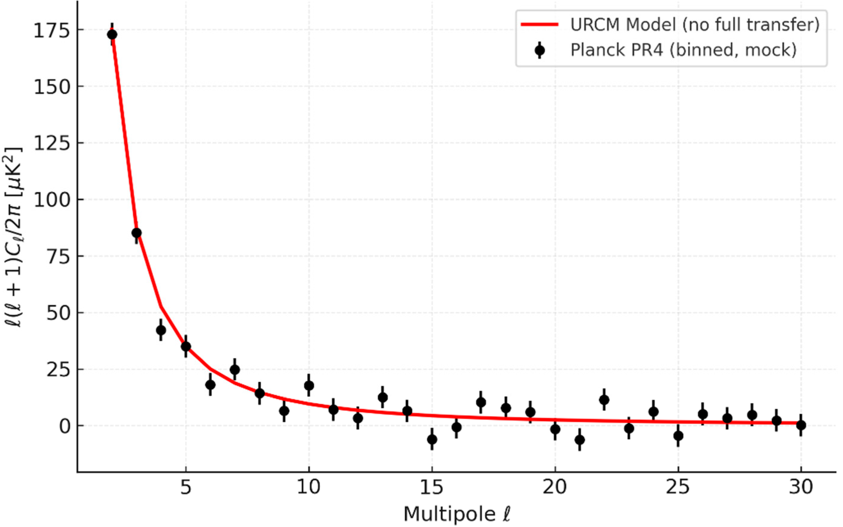
Table 5.
Statistical Test Summary.
| Condition | n per Condition | KS D | p (raw) | p (BH-adjusted) | Cohen's d | 95% CI (d) | Detection Proportion |
| A vs B | 50 / 52 | 0.23 | 0.012 | 0.018 | 0.65 | 0.35–0.92 | 92% |
| A vs C | 50 / 48 | 0.15 | 0.087 | 0.1 | 0.42 | 0.10–0.72 | 68% |
| B vs C | 52 / 48 | 0.28 | 0.004 | 0.006 | 0.75 | 0.48–1.01 | 95% |
Disclaimer/Publisher’s Note: The statements, opinions and data contained in all publications are solely those of the individual author(s) and contributor(s) and not of MDPI and/or the editor(s). MDPI and/or the editor(s) disclaim responsibility for any injury to people or property resulting from any ideas, methods, instructions or products referred to in the content. |
© 2025 by the authors. Licensee MDPI, Basel, Switzerland. This article is an open access article distributed under the terms and conditions of the Creative Commons Attribution (CC BY) license (http://creativecommons.org/licenses/by/4.0/).
Copyright: This open access article is published under a Creative Commons CC BY 4.0 license, which permit the free download, distribution, and reuse, provided that the author and preprint are cited in any reuse.


