Submitted:
04 August 2025
Posted:
06 August 2025
You are already at the latest version
Abstract
This paper presents a systematic approach for rapid assessment of the performance and robustness of linear control systems through geometric analysis in the complex plane. By combining indirect performance indices within a defined zone of desired performance in the complex s-plane, a connection is established with direct performance indices, forming a foundation for the synthesis of control algorithms that ensure root placement within this zone. Analytical relationships between the complex variables s and z are derived, thereby defining an equivalent zone of desired performance for discrete-time systems in the complex z-plane. Methods for verifying digital algorithms with respect to the desired performance zone in the z-plane are presented, along with a visual assessment of robustness through radii describing robust stability and robust performance—representing performance margins under parameter variations. Through parametric modeling of controlled processes and their projections in the complex s- and z- domains, the influence of the discretization method and sampling period - as forms of a priori uncertainty is analyzed. This paper offers original derivations for MISO systems, facilitating the analysis, explanation, and understanding of the dynamic behavior of real-world controlled processes in both the continuous and discrete-time domains, and is aimed at integration into expert systems supporting control strategy selection.

Keywords:
Г-sector
; Q-box
; robustness
; discretization
; geometric analysis
; s-plane
; z-plane
; assessment
1. Introduction
Modern control methods and algorithms lead to increased efficiency and performance of control systems by improving control performance in production processes. Achieving such improvement critically depends on the study and modeling of real controlled processes whose performance is targeted for enhancement [1,2].
The introduction of models employing intelligent solutions for parametric modeling of real-world processes [3] currently fails to provide designers with sufficient explanation or understanding regarding the combination of real parameters and the generation of control models under parametric uncertainty.
The work in [4] addresses this issue by proposing a methodology for the description, analysis, and control of systems with unknown or varying parameters, using an H∞-based framework, μ-analysis, sensitivity analysis, and worst-case approaches. However, this work remains abstract and analytical in nature, focusing primarily on continuous-time systems. Modern industry, in contrast, demands integration with visual tools that allow intuitive and rapid adaptation of algorithms or decision-making.
Moreover, the simultaneous research of uncertainties arising from both the discretization method used and the influence of the sampling period is scarcely addressed in scientific literature. For example, [5] explores how changes in the sampling period lead not only to changes in the "radius" but also in the "center" of parametric sets, turning the problem into a complex robust control challenge. Reference [6] examines various discretization methods (ZOH, Tustin, Euler, Adams, etc.) and how their selection results in differences in accuracy, delay, overshoot, and stability in permanent magnet drive systems.
Conversely, feeding parametric models into intelligent systems—even those equipped with expert knowledge—for the purpose of generating or selecting control algorithms usually fails to achieve a meaningful improvement in the properties of the real-world controlled process. This is often due to insufficient accumulated data and/or data collected from samples containing errors that the expert system cannot detect.
As a result, a gap remains between theoretical scientific norms and their transformation into usable information for designers who rely on expert systems to save time, effort, and human resources. Therefore, there is a need for an approach that combines the analytical capabilities of modern control theories with the industry's demand for fast and reliable decision-making in the control of complex processes and systems.
1.1. Brief Overview
The study of real-world processes and/or control systems requires an integrated approach with synergistic action, built upon three foundational pillars. The results of such an approach can be utilized by modern industry for the design of advanced control algorithms. The first pillar is the classical component — the complex s- and z-domains and their associated tools for analyzing stability and control performance. The second pillar is the modern component, which encompasses robust control tools, particularly in the manipulation of parametric spaces using graph-analytical relationships for tracking performance. The third pillar is the implementation of both classical and modern theory in the discrete-time domain, aiming for consistency and uniqueness of the resulting solutions in both continuous and discrete-time representations.
This work is inspired by foundational studies [7,8,9,10,11,12,13,14] that aim to build a modern perspective on the analysis and design of control systems under uncertainty, with a focus on stability, robustness, and the applicability of classical and contemporary methods in these areas.
The classical works by authors such as [7,8,9] present the fundamental concepts of control theory, including stability, root locus, frequency-domain analysis, and state-space modeling. These sources offer both theoretical depth and practical examples, making them widely adopted in academic and engineering communities.
Contemporary studies, such as those in [10,11] examine robust control under parametric uncertainty and introduce structured methodologies for the analysis and synthesis of systems that remain stable under parameter variations. These works represent a transition from classical to robust control, with an emphasis on guaranteed stability. Specialized studies, such as [12], lay the foundations for robust root locus analysis and highlight the potential for geometrically interpreting the stability of uncertain systems. Similarly, [13] apply LMI-based methods for robust pole placement, which are particularly relevant to the design of discrete-time and second order control systems.
Additionally, the study in [14] demonstrates how control theory finds real-world application in energy systems (e.g., wind energy), integrating engineering principles with sustainable design under conditions of uncertainty.
Taken together, these sources form a comprehensive body of knowledge — from classical foundations, through the development of robust theory, to their practical application in industrial systems. They provide the context for a modern approach in both discrete and continuous domains, where graph-analytical methods and root locus techniques can be adapted for uncertainty analysis, not only in system parameters but also in the structure of discretization itself.
Numerous authors in recent publications apply the root locus concept to analyze process behavior under parameter variations.
In [15], the influence of parameter changes on frequency stability in systems with virtual synchronous generators is analyzed using root locus methods in the complex plane. Graphs are presented to illustrate how control parameters affect the stability of the control system.
Reference [16] focuses on the design of robust PIR controllers, using stability boundary analysis methods. Mathematical derivations and plots are presented to show how control parameters influence the stability of the closed-loop system.
In [17], a novel combined technique is proposed, incorporating ACM and PI controllers, based on root locus tuning. A small-signal model of a DC microgrid system is developed, analyzing how variations in control and system parameters affect system dynamics.
1.2. Brief Comparison and Explanation
Most scientific sources focus individually on either the s- or z-domain, without providing a comparative transition between the two based on discretization methods and sampling time [18,19]. In classical literature, performance indices in the time domain, frequency domain, and complex plane are typically examined independently for analysis purposes, often lacking visual-graphical toolkits that facilitate the selection of control strategies ([20,21]).
While most classical and modern studies address parametric uncertainty, the uncertainty arising from the discretization process itself is rarely analyzed [22,23]. Robustness is also commonly evaluated only within a single domain, with a focus on a specific class of uncertainty, leaving open questions about the system's unambiguous behavior in other domains [24,25,26,27].
Article [28] presents an innovative geometric transformation aimed at facilitating the analysis of discrete-time systems through a mapping of the z-plane into a pseudo s-plane. However, it does not incorporate a robust perspective based on parametric analyses and graph-analytical methods for evaluating the sensitivity and stability of systems under parameter variations. A clear and unambiguous connection between the continuous s- and discrete z- domains is not developed.
Reference [29] discusses interval polynomials with coefficients varying within predefined bounds, focusing on the stability of polynomial families using a graph-analytical approach based on extended root locus theory. Although the topic addresses stability under uncertainty, it does not apply formalized robust methods from modern control theory, such as sensitivity analysis or worst-case evaluations.
In [30], an extended root locus is introduced, allowing for simultaneous variation of multiple coefficients. It demonstrates how to select values that ensure the stability of the entire polynomial model by tracking trajectories in the root space. However, it lacks integration of analysis between the continuous s- and discrete z- domains and does not apply modern robust metrics.
Reference [31] research the stability of Hurwitz polynomials through combinations of orthogonal polynomials and recurrence relations, offering constructive methods for generating stable families under parametric uncertainty. However, it does not address the relationship between the s- and z-planes.
In [32], stability conditions are proposed for convex combinations of polynomials, focusing on the stability of families through geometric and structural approaches. Yet, graph-analytical techniques for root trajectory tracking and transitions between continuous and discrete time are not considered.
Study [33] deals with fractional polynomials and complex types of uncertainty (interval, affine, multilinear), applying tools such as the Kharitonov theorem and edge theorem for stability analysis. Nonetheless, it lacks focus on classical root locus theory and its direct application for controller synthesis with a clear distinction between the s- and z-domains.
Reference [34] develops a stabilization methodology under uncertainty by focusing on dominant roots within interval systems, but it does not explore the discrete domain or interpret robustness.
Finally, [35] introduces a toolbox primarily focused on continuous-time frequency methods, which does not offer extended support for discrete-time systems.
1.3. Research Aim
The aim of the present study is to develop an integrated approach that provides a more comprehensive understanding of the overall dynamics of processes or control systems and supports control strategy selection by designers. Additionally, the graphical and analytical insights generated by this approach can contribute valuable data for the effective training of expert systems.
To achieve this objective, performance zones are defined—regions in which the characteristics of real-world processes must lie—through original derivations linking control performance properties and indicators in the complex s- and z-planes. Parametric models of controlled process uncertainty are developed, and their positioning in the complex domain is examined under both continuous and discrete-time representations.
The newly derived graph-analytical relationships offer guidance for the well-grounded selection of control algorithms and their subsequent digital implementation, establishing a meaningful collaboration between theory and practice. This theoretical framework ensures the development of control algorithms that are relevant and effective in terms of performance, both in continuous and discrete-time domains.
As part of a modern approach to control and performance analysis, the study introduces an original method for robustness evaluation in the complex s-plane, using analytical links between the frequency domain and the root locus. A parallel is drawn with the continuous-time frequency domain in the case of non-parametric uncertainty, and with the discrete-time frequency domain in the case of parametric uncertainty.
The uncertainty related to the sampling period is also modeled in an original way using methods in the complex z-plane, with the aim of enabling proper selection and tracking of its impact on control performance.
2. Gamma Regions
2.1. Definition of the Performance Region in the -Plane
The desired control performance of processes is specified through criteria formalized by indirect performance indices in the complex domain—specifically, in the root locus of the closed-loop system, the, plane, through the transition , denoted as the , (1) and in the frequency response domain through the transition , . The performance specifications in the frequency domain are also of an indirect nature (gain and phase margins, delay margin, resonance peak, bandwidth, etc.), but they are not the focus of this study.
where: – undamped natural frequency, – damped natural frequency, - damping ratio, – stability degree.
The Indirect Performance Indices are not directly measurable from the physical system. Their determination requires approximation, mathematical modeling, or system identification procedures. They represent abstract characteristics of a dynamic model based on the system's transfer function, rather than directly observable quantities. The general case of describing the complex variable assumes that , which defines the complex plane and enables the application of the concept of dominant roots of a closed-loop control system. The concept of dominant roots originates from the prototype of a second order closed-loop system, given by, (2).
where the damping ratio (3) and the undamped natural frequency (4) are dimensionless quantities.
- real physical parameters of the controlled process.
Physically meaningful values of the damping ratio satisfy the condition . The concept of dominant roots encompasses all possible dynamic states that can describe a real control process. Therefore, it is essential that the entire desired dynamics and behavior of real processes can be mathematically represented and graphically displayed in the complex plane, to identify suitable control algorithms and enable proper analysis of the solutions obtained. The coordinates of the roots from (2) are given by (5) and define the indirect performance indices in the complex plane, whose graphical combination forms the zone – region, see [10], Figure 1. The coordinates in (5) refer to the case when the damping coefficient lies within the range , as this case contains the most important analytical conclusions. The zone represents the desired performance region in which the roots of the closed-loop system (the control algorithm and the real process) must be located. The specifications defining are mathematically derived through the following geometric relations (6)– (9), see Figure 1.
The relationship between the indirect performance indices and the direct performance indices of transient processes (10) is expressed through the time-domain response of the second-order control system prototype (11)
where the overshoot (12), settling time , (13), time of the first peak , (14) and rise time (15) are given by the expressions (12)– (15).
The desired performance zone can be refined with a lower bound and an upper bound of the indirect performance indices . Its boundary is described by the following expression (16), Figure 1
The definition of and creates a premise for a new class of problems that require a control algorithm to ensure that the closed-loop system roots are located within the region.
2.2. Defining of the Performance Region in the –Plane
The – region has its counterpart in the complex – plane, . For this purpose, the necessary expressions for the transformation from the plane to the plane. The mathematical description of the complex variables and is given by equations (17) and (18):
where the modulus is given by , and the argument is:
where the modulus is , and the argument is .
The relationship between the two complex variables and is given by . Equations (19)– (21) are written as follows.
where is the sampling period, [t].
From equations (19)– (21), it follows that for known real and imaginary parts of the complex variable (22) the modulus and argument of the complex variable can be found as in (23).
To define the performance region it is necessary to use the relations (22) and (23) and find the geometric equivalents through mathematical expressions of the performance specifications (6)– (9), which determine the indirect performance indices , (1). The five most characteristic cases are considered:
, – for
The mathematical correspondence is given by (24)
Expression (24) describes circles in the - plane. For and modulus of the complex variable , the unit circle in the - plane is obtained. When and modulus the degree of stability, , is defined (see Figure 1), with the corresponding circles located inside the unit circle and centered at () in the plane.
- , – for
The analytical relationship between the - and - plane is given by the equation (25)
The relation (25) shows that a line with fixed frequency between in the plane is transformed into a ray with fixed angle in the plane, but with a variable modulus .
, – for
The required expressions are given by (26).
It can be seen from (26) that the two lines at , in the plane transform into a single line located at in the plane.
- – for
The relationship between the - and - plane is obtained using the expressions (27).
Relation (27) shows that the straight line forming an angle with slope which determines the damping ratio in the - plane, corresponds in the - plane to a logarithmic spiral located inside the unit circle.
- , – for
The mathematical correspondence between the two planes and is given by equation (28).
Equation (28) shows that the shape of the semicircles defined by in the - plane transforms into a teardrop-shaped figure in the - plane, located inside the unit circle. Figure 2 illustrates the desired performance region , obtained by applying expressions (24)– (28).
The representation of the performance region in the discrete-time domain is a necessary condition for analyzing the correspondence between the and plane as well as for evaluating the performance of control algorithms and control systems designed in the continuous-time domain when, in real operational environments, the signals are discrete in time.
3. Robustness in the s-Plane
Defining the performance regions in the and planes raise questions related to the concepts of robust stability and robust performance through the lens of the root locus plane. In the present study, the concepts of robust stability and robust performance are originally interpreted from the root locus plane, with conclusions based on the most common case of dominant closed-loop roots , (5), the performance region from Figure 1, and a non-parametric description of uncertainty in the real process model (29).
Equation (29) shows the relative error between the real process and its model . Equation (29) is also known as the multiplicative uncertainty model in robust control approaches. It is known that the sum of the sensitivity function and the complementary sensitivity function is given by (30):
In the ideal case, which is a mathematical abstraction , , achieving insensitivity of the closed-loop system to the uncertainty (caused by modeling errors, changes in the operating point, etc.) and perfect tracking of the reference signal . In real applications, the goal of control algorithms is for the closed-loop system dynamics to closely follow the reference input . Therefore, conditions for robust stability (31) and robust performance (32), are formulated. These conditions are well interpreted in the frequency domain , as they are defined through magnitudes that reflect the system's sensitivity to disturbances acting on it, which need to be attenuated.
3.1. Calculation of Sensitivity Functions and .
For a given configuration tuning of the closed-loop system , its dominant poles are fixed in the complex plane. These poles may be real and equal, real and distinct, complex conjugates with a nonzero real part, or purely imaginary with a zero real part, and may be located at the origin of the coordinate system in the complex plane. The position and the resulting system performance depend on the value of the damping ratio , (). In the complex plane, the magnitude of the closed-loop system poles , (33), considering the damping ratio is given by expressions (34)– (37):
Equations (34)–(37) for the magnitude of the closed-loop poles , show that the magnitude of the sensitivity function depends on how quickly the system responds to input stimuli, i.e., on the undamped natural frequency , of the control system, assuming a fixed value of the damping ratio . It is important to note that the real part of the closed-loop pole magnitude , is always , only when is it possible for . For the complementary sensitivity function its magnitude is given by equation (38), and for the sensitivity function its magnitude is given by equation (39), considering equation (30).
Expression (38) represents the control system's gain, expressed through . The magnitude can be interpreted in terms of distances and from a control point at a significant system frequency , (41), located on the imaginary axis , to each of the pole’s , (40). This control point is often , since the frequency is close to the resonance frequency, at which . Frequencies considered significant for the control system are typically those located one or two decades around the crossover frequency of the real process model , (41).
Table A1 presents the calculated values of и пo (40), using equation (40), for various configurations of dominant poles and significant frequencies , [rad/s], з in order to draw conclusions about .
- If the control point frequency is close to the dominant poles and the distance to the imaginary axis is small, the magnitude becomes large, and the control system will exhibit oscillatory-damped transient responses.
- If the control point is far from the poles , is smaller, and the control system will show faster time response at that frequency .
In analyzing it is important to note that the sensitivity function is inversely related to the characteristic polynomial of the closed-loop system , where is the open-loop transfer function of the control system, as defined in (42).
indicates that for a fixed tuning of the closed-loop system , and hence for given poles (obtained from a specific open-loop system ) the magnitude of is also fixed. The root locus of the inverse sensitivity function shows the position of the open-loop poles of the system , i.e., the starting point of the root locus when . An important aspect when studying the robustness of systems through the sensitivity functions and their magnitudes and in the complex plane is the value of the natural frequency .
Two cases are distinguished:
- When , the magnitude of the closed-loop system tends to approach 1 more rapidly, and the system sensitivity remains low for a fixed damping ratio . However, if the value of , where changes, the real part of the dominant poles decreases, leading to an increase in the magnitude of the sensitivity function , as shown in Table A1.
- When , the magnitude , regardless of the value of the damping ratio , which results in , also shown in Table A1.
The conclusions drawn regarding the significant frequencies and the dominant poles as well as the relationships between and , together with the calculations from Table A1 concerning the sensitivity function and the complementary sensitivity function , enable their graphical representation in the complex plane shown in Figure 3. The geometric interpretation of the magnitudes of and , calculated using equations (38) and (39) through the distances and , (40) is presented in Figure 3 for values of , in the cases and , where , [rad/s], and , [-], with a fixed damping ratio , [-].
A control point is marked in pink at , for which the required calculations of and are shown
3.1.1. Discussion
The magnitudes of the sensitivity function and the complementary sensitivity function play a key role in control theory. When there exists a significant frequency that is much greater than the system’s natural frequency , i.e. , the control system is unable to track its reference input. In such a case, the entire error is passed to the output of the closed-loop system, and the sensitivity to disturbances and uncertainty, represented by increases up to 1, in accordance with equation (30).
Based on the conducted studies regarding robustness in the complex plane, the following general conclusions can be made, considering expressions (38) and (39)
- The dominant roots of the closed-loop system , which characterize the control of the real process must be located sufficiently far from every point , on the imaginary axis so that the magnitude remains acceptably small to compensate for the uncertainty .
- If the magnitude is larger, this leads to oscillations in the transient responses, a general reduction in system stability, and the robustness condition (31) will be violated.
- If are located close to the points on the imaginary axis , the distances and become small, i.e., is large, and stability decreases. On the other hand, this implies that will be small, (30), which is an indication of insensitivity.
These trade-offs and the pursuit of robustness require a broader perspective of the complex domain, referred to as a compromise, which demands the following:
At low frequencies, , the sensitivity function should be small to eliminate steady-state error and to suppress disturbances .
Simultaneously, the complementary sensitivity function should be large to ensure proper tracking of the reference input . Conversely, at high frequencies, , should be small to provide noise attenuation and preserve system robustness against high-frequency uncertainties.
This compromise forms the core of robust control design and is crucial for balancing performance and robustness across the entire frequency spectrum.
3.2. Robust Stability and Robust Performance (
An original geometric interpretation of the conditions for Robust Stability and Robust Performance , defined in the frequency domain by equations (31) and (32), but interpreted from the perspective of the complex plane is presented for control points corresponding to the essential frequencies , [rad/s], with values of , [-], and a fixed damping ratio , [-]. This interpretation is visualized in Figure 4, Figure 5, Figure 6 and Figure 7, based on data from Table A1.
A complete analysis was carried out using all combinations of the complex parameters and , where , and , for the entire range of essential frequencies .
Around the dominant poles circles are drawn with radii equal to the values of and , denoted and . These radii are obtained for , where the magnitudes of and are calculated using equations (38) and (39). The black circles around have radii equal to , denoted and represent the uncertainty region within which the poles may shift in the presence of model uncertainty .
3.2.1. Discussion
Figure 4 was generated for the case Under this lower uncertainty level , the analyzed process maintains stability and performance when the dominant poles are located farther away from the imaginary axis . Poles located closer to the imaginary axis led to increased system sensitivity and as seen in Figure 4, the system may lose both robust stability , and robust performance , at specific frequencies (see Table A1). This shift in system dynamics is caused by the low damping ratio , which results in highly oscillatory transient responses and degraded indirect indicators of stability. As the frequency and consequently increases, the number of frequencies at which robust stability is guaranteed decreases (Table A1). Additionally, there is an intersection of the circles defining with the imaginary axis . Typically, at higher damping ratio values the system retains stability under uncertainty for all frequencies, , (highlighted in green), and robust performance is also achieved across the entire frequency range (highlighted in blue). For configurations of the circle radii defining robust stability, robust performance, and uncertainty under , condition (43) holds (43)
This implies that the system has a robust performance margin which can be calculated using equation (44)
If the value of equation (44) is negative, conditions (31) and (32) are violated, If the value is positive, it indicates that the system has a positive robust performance margin , as per equation (44).
Figure 5 was obtained for the combination . The same conclusions made regarding Figure 4 apply here. The reduction of the reference input decreases the radii of the circles , which describe for all frequencies . The difference in this case arises from the robust performance margin , which for is given by (45), and for given by (45), and for the conditions (31) and (32) may be violated:
For has a value of 0.5, and the blue circles coincide with the circle describing . With the increase of the natural frequency the margins for robust stability and robust performance decrease (see Table A1). Changing the reference input affects the weighting of the sensitivity function , where smaller values of provide better robust stability and robust performance .
Figure 6 was obtained for the case . The uncertainty is large, corresponding to a 120% variation in the parameters of the control process. This situation shows that the conditions for robust stability and performance (31) and (32) are not satisfied for some frequencies , as shown in Table A1. With increasing values of the damping ratio , and respectively with the dominant roots moving away from the imaginary axis, the process exhibits better dynamic properties. However, conditions (31) and (32) are still violated for important frequencies . The intersection of the imaginary axis by the circles colored red and pink, which corresponds to the lack of robust stability and performance, represents a risk zone for loss of system stability.
Figure 7 was obtained for the combination . For this particular combination, as shown in Figure 7 and Table A1, the process is characterized by robust stability , but robust performance is not present. This fact is explained by the increase in the scaling factor of the sensitivity function through . Additionally, loss of stability of the process is possible, since the circles for which condition (32) is not satisfied intersect the imaginary axis in the complex plane.
In summary, the following conclusions can be drawn:
- A quick engineering analysis when applying the proposed strategy for evaluating robust properties from the complex plane boils down to checking the radii of the circles. Larger radii and indicate smaller margins of robust stability and robust performance , as seen in Figure 6 and Table A1. The intersection of circles obtained when conditions (31) and (32) are violated is an indicator of a potential loss of stability of the system/process control (classical analysis is required for confirmation).
- Visualization of regions defined by circles in the complex plane allows searching for solutions that will reduce the radii and n order to bring the regions into the desired performance region. This shows that the study of robust properties in controlling real processes from the root locus plane is a feasible approach, which can be easily automated and provide information to expert systems and designers for preliminary and/or final selection of a control algorithm.
The representation of as a non-parametric uncertainty, like well-established methods in the frequency domain, is applicable for real processes with continuous mathematical descriptions. When discrete-time modeling of the control process is required, a parametric description of the uncertainty is used to reduce the introduction of additional inaccuracies during the design of the control algorithm.
4. Parametric Uncertainty Models
4.1. Q−box. Parameters Uncertainty
The geometric interpretation of robustness of control systems for real processes from the complex plane can be represented through parametric models of uncertainty, expressed by forming a [10]. Every mathematical model of a real process (29) involves uncertainty due to known factors. This uncertainty, error, or multiplicative uncertainty in the real process can be described only by the real parameters of the controlled process (46)
where are parameters (fixed but with unknown values within given bounds).
is the set of admissible values that the parameters can take. The parameters of the process carry information about the real characteristics of the control process. They are obtained from the description of the real process by differential equations based on physical, chemical, mechanical, and other laws. In terms of automation represent gain coefficients , time constants , which can appear in different combinations, ratios, and models of the real process dynamics. The real parameters from (4) become functions of , upon variation, i.e. , , where and and the real process dynamics can be described by (47)
A canonical form of describing the dynamics in control systems with parameters , (is assumed (either through a differential equation or through the transfer function (48), to indicate uncertainty in the parameters of the control process.
This creates convenience in the analysis of parametric uncertainty, since the parameters и express the relationship between the real gain coefficients and the time constants and carry information about the actual physical structure of the process, (49).
where is a function reflecting the structure of the control process.
The parameters are dimensionless quantities, , [-], (50).
The number of parameters allows graphical visualization of their uncertainty through a . Figure 8 shows the region for different numbers of parameters .
The represents a parametric model of the uncertainty in the parameter space . It is unified because its shape depends only on the parameters . Differences between various processes arise from the size of the , which is determined by the specific numerical values of the parameters . For parameters, were, , the shape of the is an n-dimensional hypercube. The provides a priori graphical information about the type and magnitude of the uncertainty in the control process. This information is the starting point for selecting a control strategy that uses passive adaptation (robustness), as the parameter variations , expressed through are present.
4.2. Generation in s-Complex Roots Plane
The formation of the – region, shown in Figure 1, raises questions related to the concepts of – stability and - performance. The test for -stability and performance reduces to analyzing the trajectories of the roots of the characteristic equation (42), , obtained under a parametric description of the uncertainty, called the , relative to the region guaranteeing the desired performance . The is an important region, as in the continuous-time case it is involved in procedures for analysis and synthesis of continuous controllers with robust properties [36].
Determining the uncertainty region in the complex plane, obtained by varying the process parameters (46), is associated with the use of the root locus method applied to variations of the corresponding interval parameter . The general form (42) of the characteristic equation of the closed-loop system under parametric uncertainty and unit negative feedback, is represented by (51).
where is the Evans coefficient, is the transfer function of the controller, and - is the transfer function of the controlled process with varying parameters.
The characteristic equation of the closed-loop system (51) takes the form (52), which is suitable for isolating the uncertain parameters.
Equation (52) needs to be modified so that the free, variable, uncertain, real parameter , is separated as the Evans coefficient , to plot the root locus for . For example, for the characteristic equation with respect to the expression (53) is obtained.
In a similar manner, the procedure is applied to all uncertain parameters . Each resulting segment of the root locus obtained in the described way (53) for represents an uncertainty region called the . The relationship between the two regions, the and the is established through the characteristic equation of the closed-loop system (52).
The following particularities must be considered when constructing the .
- For values of the root locus enters the class of negative root locus ().
- When modifying equation (52), it is possible that equation (53) violates the physical realizability condition, resulting in - that is, the order of the numerator polynomial exceeds the order of the denominator polynomial in the open-loop transfer function. Therefore, instead of using , as the varying parameter, the Evans coefficient function is represented by .
- In case of a nonlinear dependence of , the usual rules for constructing the root locus are not applicable.
4.2.1. Numerical Example
Further in this study, the formation of the for parameters with is considered. The characteristic equation of closed loop control system of a real process is described by (54)
The nominal values of the dynamic parameters of the control process — time constants and gain coefficient are respectively: , and . For the purpose of the study, a proportional controller with proportional gain is assumed in the system. The parametric uncertainty in the control system arises from a 20% variation in the three dynamic parameters of the process from their nominal values, i.e. , (55) , , ,
Equation (52) takes the form of (56).
- Discussion
The following possible scenarios of combinations of the parameters are considered:
- 1.
- Case 1 -
Equation (56) takes the form of (57).
For generating the , equation (52) is modified into a single equation (58):
Figure 9 shows the region. The appears as a line since the parametric uncertainty is present in only one parameter of the control process.
- 2.
- Case 2 -
Equation (56) takes the form of (59).
For generating the , equation (52) is modified into two equations with two uncertain parameters and , given by (58) and (60):
Figure 10 shows the region. The zone represents a combination of a line corresponding to the third pole, since it is real, and a two-dimensional figure corresponding to the complex-conjugate poles, as the parametric uncertainty is present in two parameters of the control process.
- 3.
- Case 3 - for , , , ,
Equation (56) takes the form:
For generating the , equation (52) is modified into three equations with three uncertain parameters, , and , given by (58), (60) and (61)
Figure 11 shows the region. The represents a combination of a line corresponding to the real pole of the process and a three-dimensional figure corresponding to the complex-conjugate poles, arising from uncertainties in three parameters of the control process.
The enables direct visual assessment of the stability of the control system. If any parts of the zone intersect the imaginary axis, this indicates that, for the corresponding combination of process parameters, , the control system will lose stability without the need for further checks. Analytically, stability can be conveniently verified using the polynomials that describe the vertices of the shown in Figure 11. This Figure 11 was selected for detailed consideration because the encompasses all other cases described and illustrated in Figure 9 and Figure 10. In this particular case, the characteristic (interval) polynomial has the form (62):
The Kharitonov polynomials [10] can only be applied when the coefficient intervals are independent. In this particular case, the classical theorem is not directly applicable, and the cannot be fully covered by combinations that include all possible stable cases. Therefore, the following coefficients are introduced: , and . Equation (62) takes the form of (63), from which the polynomials whose solutions satisfy , corresponding to the vertices of the take the forms (64)– (71), shown in Figure 12.
Some authors refer to the as the robust root locus [12], if the е is located in the left half of the complex – plane, as shown in Figure 12. For the case illustrated in Figure 12, the region is constructed, with its boundary marked by a pink line, (16). For the analysis of – stability and – performance it is sufficient to use the polynomials (63) and check the position of the current roots. In this particular case, both – stability and – performance, are present since the is entirely located within the desired performance range. For comparison, in Figure 12, a yellow circle with radius represents uncertainty as a non-parametric model centered at the nominal values of the parameters . Noticeable differences can be seen between the parametric uncertainty represented by the and the non-parametric uncertainty in the parameters of the control process .
4.3. Generation in z-Complex Roots Plane
In the digitization of control algorithms, there is no guarantee that the robustness and stability of the control system will be preserved, since discrete approximations of the complex operator are applied. It is crucial in the digital implementation of control algorithms that the region is accurately and correctly mapped into the discrete domain. Accounting for the effects of aliasing and warping, which are inherent in discrete transformations, as well as ensuring the accuracy and stability of the resulting discrete system, is an essential step.
Aliasing is a phenomenon where high-frequency components of the continuous system appear as low-frequency components in the discrete implementation when the sampling frequency is chosen too low. This violates the Nyquist–Shannon sampling theorem (also known as the Kotelnikov–Shannon theorem in Eastern literature) and leads to signal distortion and information loss during the reconstruction from discrete to continuous signals.
Frequency warping is a consequence of the bilinear transformation, which changes the relationship between the discrete frequency and the continuous frequency according to . It distorts the frequency axis , but prevents aliasing by avoiding frequency overlaps. To mitigate warping effects, a pre-warping correction is applied for the critical frequency relevant to the process.
4.3.1. Numerical Example
In the present study, a comparative analysis is carried out using three discretization methods: (Impulse Invariance), (Zero-Order Hold) and (Bilinear Transform). Discrete transformations of the characteristic equations (58), (60), and (61) are applied using all three methods to discretize the control process described in Section 4.2.1, with the goal of generating the .
These three discretization methods were selected because, in industrial practice, each offers specific advantages in the implementation of control algorithms:
provides a good approximation of continuous-time behavior in the frequency domain, offers accurate representation of transient responses in continuous-time systems, and yields realistic modeling of continuous-time behavior with sample-and-hold effects.
is suitable for systems or real processes with low frequencies, which are characterized by slow transient responses (72). After discretization, the control system responds to an impulse in the same way as the original continuous system. However, it is prone to aliasing when higher-frequency components are present (i.e., in faster control processes).
is commonly used in the discretization of control algorithms because it realistically reflects the holding behavior of DACs (Digital-to-Analog Converters), as shown in equation (73). It acts as a low-pass filter; although it attenuates high-frequency components, it still allows aliasing to occur.
method does not prevent aliasing but preserves system stability by mapping the to the . This mapping distorts the frequency scale but maintains stability, as shown in equation (74). It is particularly suitable for digital implementation of controllers, as the continuous frequency range is compressed into the finite discrete interval .
where – sampling period, [t], variable in the domain after applying the bilinear transformation, – pseudo-frequency defined as .
- Discussion
Figure 13, Figure 14 and Figure 15 show the generated , regions obtained for the following parameter combinations:
Case 1 -, see Figure 13.
Case 2 - , see Figure 14.
Case 3 - for , , , , see Figure 15.
Discretization of equations (58), (60), and (61) has been performed using the three methods (72)– (74), for the following sampling periods: .
In Figure 13, Figure 14 and Figure 15, the parametric uncertainty is illustrated in the plane, represented by the . The following expression can be written (75)
That is, the discrete equivalent of the , namely the s obtained using , and , discretization methods, as defined in equations (72)-(74).
Depending on the number of varying parameters , the assumes a shape analogous to that shown in Figure 8, transferred through the characteristic closed-loop equation, (52) as depicted in Figure 9, Figure 10, Figure 11 and Figure 12. This shape is preserved during discretization, with the key distinction arising from the sampling period and the discretization method applied to generate it. As observed in Figure 13, Figure 14 and Figure 15, when the sampling period , is small relative to the system dynamics (see (55)), the differences between the discretization methods (72)– (74) are minimal or practically negligible. With an increase in particularly beyond =0.2 significant differences emerge between the discretization methods, as summarized in Table A2. The most pronounced deviations from the continuous-time system behavior are seen with the , method, due to the frequency warping introduced in the domain, as described by equation (74).
The performance range in the z-plane shown in Figure 16, is obtained through the discretization of the continuous-time performance range , defined in Figure 1, using the three methods considered in this study (72)– (74). This relationship can be expressed as (76)
- Discussion.
Depending on the discretization method (72)– (74) and the sampling time , the performance range defined in Figure 2, also changes, as shown in Figure 16.
At a small sampling time the zones for the different methods (, and ) are almost identical, which indicates that there will be minimal difference in the dynamic behavior of the control process. This means that at high sampling frequency the discrete-time system closely approximates the behavior of the continuous-time system.
As the value of increases, the begin to diverge more significantly, and the difference between the method and the methods becomes more pronounced—especially at , к where the divergence is clearly visible in Figure 16. The transformation causes greater frequency distortion, which affects the shape and position of the . Table A2 shows the calculated boundaries for the different methods and sampling periods .
At small there is no significant difference between the discretization methods (72)– (74), and any of the three methods can be used, as system stability is preserved. The distortion introduced by the е method is negligible at low . However, at higher values of a visible difference between the methods emerges. While system stability is still maintained, the dynamic behavior changes, and the distortion from the method becomes significant. In such cases, the choice of discretization method becomes a critical step.
4.3.2. Study of the Influence of Sampling Time
The sampling period and its variation can be considered uncertain, since different values yield different results, as shown in Table A2. The maximum allowable sampling period с is determined by the Kotelnikov–Shannon theorem, while the minimum is limited by the computational capabilities of the PLC, (77) and (78).
For example, in the specific case, the crossover frequency of the nominal process described by (55) is rad/s. We assume (78), i.e., the variation interval is described by (79).
Therefore, this a priori known variation (79) can be modeled and used to ensure insensitivity with respect to the sampling period , considering the entire context such as the discretization method, process dynamics, and closed-loop system stability.
This can be achieved by isolating the sampling period ,. as an Evans coefficient in the discrete characteristic polynomial (52). For the three methods considered, this is only possible with the method (see section 4.2), since in the and methods, the sampling period is nonlinearly dependent and cannot be separated as a free variable parameter. The discrete realization of the characteristic polynomial (52), modified to isolate the Evans coefficient, has the form (80).
Figure 17 shows the root locus for , where the sections corresponding to sampling periods , are marked with yellow dots, and the range of allowable variation for , under the three-parameter uncertainty is indicated with pink dots.
From Figure 17, the sampling period can be conveniently determined so that it lies within the range и ensuring correct reconstruction of the continuous signal. This interval guarantees that the system frequencies remain well away from the aliasing zone , and the distortion introduced by the bilinear () transformation will be minimal.
4.4. Generation in a Frequency Domain Design Template
regions also have their representation in the frequency domain. For continuous-time systems, this is obtained through the substitution and for discrete-time descriptions, through the substitution . The method provides a unique frequency spectrum in the discrete domain via the – domain (74), which allows the entire mathematical apparatus for frequency-domain analysis and synthesis of continuous systems to be applied to discrete systems without limitations related to information loss during signal reconstruction for sampling frequencies . The drawback of this approach is phase distortion at high frequencies, but by using a pre-warping frequency (in the article, the arithmetic mean of the critical frequencies is used) the global distortion characteristic for high frequencies is compensated (for the purposes of this study).
4.4.1. Numerical Example
The article analyzes the in the discrete frequency domain, obtained using the three discretization methods (, и ). However, due to (74), the main conclusions for interpreting robustness are drawn from the approximation obtained via the method. The are constructed in the Nichols plane (), as it is a fundamental tool for performance analysis and is highly applicable in the synthesis of robust controllers, for example through QFT [1,14].
- Discussion
The are constructed under the following conditions: for , , , , , by discretizing equations (58), (60), and (61) using the three methods (72)–(74) (including correction for distortion) and with sampling periods . These are shown in separate figures from Figure 18, Figure 19, Figure 20, Figure 21, Figure 22 and Figure 23, for a vector of frequencies relevant to the process .
In Figure 18, Figure 19, Figure 20, Figure 21, Figure 22 and Figure 23, the continuous system (labeled as ) is included to enable comparative analysis. When using the discretization method and a small sampling period , he is corresponding discrete equivalent of the process closely approximates the continuous system (see Figure 18, Figure 19, Figure 20 and Figure 21). For larger sampling periods the lines forming the с begin to disintegrate or experience phase discontinuities (so-called "unexpected jumps"). This behavior is characteristic of method, especially when the system has poles/zeros near the stability boundary (see Figure 22 and Figure 23).
For the discretization method, it is typical for the amplitude of the process to be preserved. However, at large values of (), the phase of the begins to lag, and its curves shift to the left (Figure 22 and Figure 23). The distortion becomes significant at higher frequencies and larger .
The м method is designed to preserve the frequency characteristics, but it introduces phase distortion, especially at higher frequencies . With the added phase correction applied in the construction of the the zone lines match much more closely with those of the , particularly at small sampling intervals (), as shown in Figure 18 and Figure 19.
At larger sampling intervals () deviations are still present, but they are smaller compared to the , method, as seen in Figure 22 and Figure 23. The specific comparison regarding the sampling interval leads to the following conclusions:
- All discretization methods are very close to the continuous-time analog of the process (Figure 18).
– Small deviations are observed in the when using the and methods (Figure 19).
discretized using starts to lag, while the one using remains accurate (Figure 20).
– Clear phase shifts are observed in the with and methods, Figure 21).
- Errors caused by the large sampling interval and discretization method become significant (Figure 22).
- The discretized equivalents of the deviate significantly from the continuous system, especially , (Figure 23).
In this specific case, it can be concluded that discretization with minimal phase distortion is achieved using the method with frequency pre-warping. The method is the most suitable for generating uncertainty templates, for instance in the QFT methodology. offers easy implementation, but only at small ((e.g. ) significant frequency distortions will occur.
4.4.2. Robustness in the Frequency Domain
For completeness of the exposition, it is necessary to visualize the parametric uncertainty of the parameters in the frequency domain, in the case of continuous-time descriptions of processes or control systems. In the frequency domain, conditions (31) and (32) for robust stability and robust performance have a well-established and widely known graphical interpretation, usually represented through the configuration of circles and the comparison of their radii [37].
Figure 24 shows the frequency response in the Nyquist plane for the process в 4.2.1 studied in Section 4.2.1 under nominal operating conditions, equation (55). For three characteristic frequencies () from the vector of essential frequencies defined in Section 4.4.1, circles are drawn with radius , and center (the corresponding frequency). These circles are marked in pink on Figure 24. The distance from the center of the circles to the point with coordinates с corresponds to the inverse of the sensitivity function , obtained as the sum of vectors of lengths 1 and , (81)
From this, the graphical verification of conditions (31) and (32) follows. If the distance is greater than the radius, the condition for robust stability (31) in (31) is satisfied, equation (82).
For robust performance (32) according to condition (32), the following must be fulfilled:
The distance from the point with coordinates to any point of each set (i.e., the distance ) т must exceed the distance from the point to the center for the corresponding frequency, reduced by the radius of the circle , that is (83)
When the uncertainty is represented parametrically via the , cube is formed from the extreme combinations of the parameters . The reflects the actual range of the frequency response, while the circles provide only an approximate boundary defined by the radius , which is a fixed relative value.
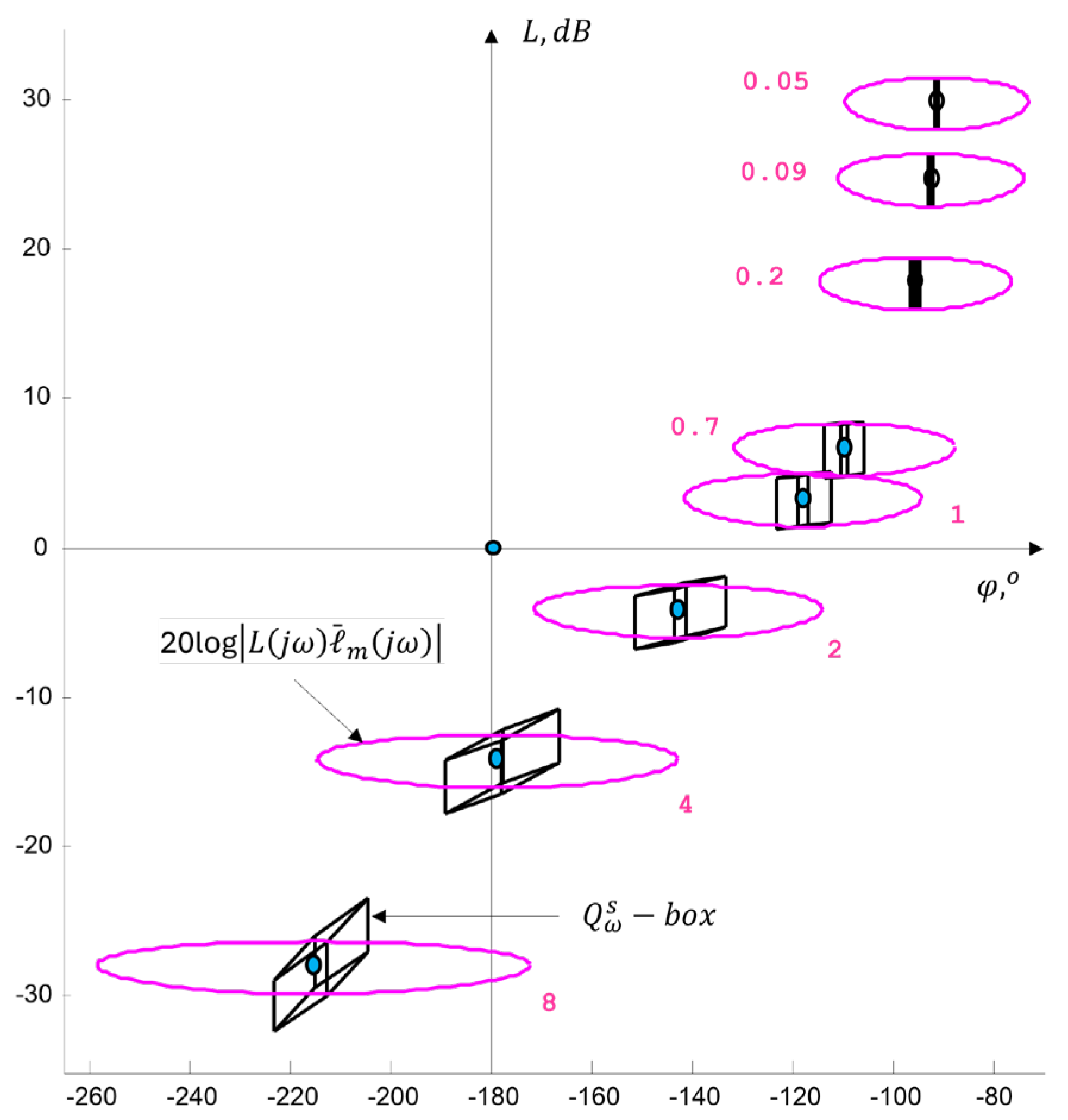
Figure 25 shows a portion of the frequency response of the process in the Nichols plane, under conditions corresponding to the graphical interpretation from Figure 24. The are templates of parametric uncertainty, which are used in the design of controllers via QFT (Quantitative Feedback Theory). For successful synthesis and to avoid introducing additional modeling uncertainty, the uncertainty in the process must be represented parametrically, as shown in Figure 25.
5. Conclusions
The article proposes a systematic approach that combines classical and modern methods for rapid engineering analysis, aimed at a better understanding of process dynamics due to the need for decision-making on control strategy.
The integration of indirect performance indices within a geometrically defined desired performance region establishes a connection with the direct performance indices and lays the foundation for synthesizing control algorithms that ensure the closed-loop system dominated poles fall within the desired performance range, going beyond the classical stability check. A discrete-time representation analogue of the region in the plane, denoted as region, is defined by deriving analytical relationships between the complex variables and , which transform the . The region is used to verify control algorithms implemented in the discrete-time domain.
The desired performance regions and enable a new approach for interpreting robust stability ( and robust performance (, traditionally formulated in the frequency domain, through geometric analysis in the complex - plane based on the location of the system roots under unstructured variation of the process parameters . A methodology for visual assessment of robustness has been developed using circles with radii , and , allowing for the calculation of a robust performance margin , under various scenarios . This approach allows for automation and integration into expert systems.
The need for digital equivalents of control algorithms requires a parametric representation of process parameter variations through the so-called . Consequently, a sequence of zones , are defined and compared, derived under varying parameters . Particular attention is given to the specific characteristics arising from the use of different discretization methods (, ) and the influence of the sampling time is examined through an original modeling approach that treats it as an a priori uncertainty. A reference is also made to a graph-analytical robustness assessment in the frequency domain, addressing unstructured uncertainty and parametric uncertainty in the process parameters .
The advantage of the proposed integrated approach lies in its direct applicability in real practice environments for rapid orientation, owing to its simple and well-formalized relationships. This simplicity does not reduce its significance; rather, it facilitates the analysis of situations arising from changes in control processes and supports decision-making regarding the selection of control algorithms or the evaluation of real process performance. The limitations of the study relate to its applicability primarily to linear or linearized systems. The discretization conditions are idealized (i.e., without noise, delays, etc.), and only the most used discretization methods are considered. The results are applicable to processes or systems with single or multiple inputs but a single output (MISO configuration).
Future developments may focus on the design of specific control algorithms based on the , aimed at ensuring guaranteed и stability and performance. Another direction involves the development of an expert system based on the visual zones, enabling automated conclusions regarding robust stability and performance. Further expansion could include extending the approach to MIMO configurations.
Appendix A

| 0.10 | 3.00 | 0.20 | 2.9021 | 3.0980 | 1.0010 | 0.0010 | 1.202 | 1.201 | |
| 0.10 | 3.00 | 0.50 | 2.9138 | 3.0870 | 1.0006 | 0.0006 | 1.201 | 1.201 | |
| 0.10 | 3.00 | 0.90 | 2.9578 | 3.0449 | 0.9993 | 0.0007 | 1.200 | 1.199 | |
| 0.10 | 5.00 | 0.20 | 4.9021 | 5.0980 | 1.0004 | 0.0004 | 1.201 | 1.200 | |
| 0.10 | 5.00 | 0.50 | 4.9137 | 5.0868 | 1.0002 | 0.0002 | 1.200 | 1.200 | |
| 0.10 | 5.00 | 0.90 | 4.9572 | 5.0444 | 0.9998 | 0.0002 | 1.200 | 1.200 | |
| 0.10 | 7.00 | 0.20 | 6.9020 | 7.0980 | 1.0002 | 0.0002 | 1.200 | 1.200 | |
| 0.10 | 7.00 | 0.50 | 6.9136 | 7.0868 | 1.0001 | 0.0001 | 1.200 | 1.200 | |
| 0.10 | 7.00 | 0.90 | 6.9570 | 7.0442 | 0.9999 | 0.0001 | 1.200 | 1.200 | |
| 3.83 | 3.00 | 0.20 | 1.0697 | 6.7909 | 1.2389 | 0.2389 | 1.606 | 1.487 | |
| 3.83 | 3.00 | 0.50 | 1.9379 | 6.5959 | 0.7041 | 0.2959 | 0.993 | 0.845 | |
| 3.83 | 3.00 | 0.90 | 3.6915 | 5.7995 | 0.4204 | 0.5796 | 0.794 | 0.504 | |
| 3.83 | 5.00 | 0.20 | 1.4675 | 8.7811 | 1.9401 | 0.9401 | 2.798 | 2.328 | |
| 3.83 | 5.00 | 0.50 | 2.5505 | 8.5297 | 1.1491 | 0.1491 | 1.454 | 1.379 | |
| 3.83 | 5.00 | 0.90 | 4.7914 | 7.5036 | 0.6954 | 0.3046 | 0.987 | 0.834 | |
| 3.83 | 7.00 | 0.20 | 3.3410 | 10.7749 | 1.3611 | 0.3611 | 1.814 | 1.633 | |
| 3.83 | 7.00 | 0.50 | 4.1539 | 10.4884 | 1.1247 | 0.1247 | 1.412 | 1.350 | |
| 3.83 | 7.00 | 0.90 | 6.3473 | 9.3259 | 0.8278 | 0.1722 | 1.079 | 0.993 | |
| 7.55 | 3.00 | 0.20 | 4.6495 | 10.5065 | 0.1842 | 0.8158 | 0.629 | 0.221 | |
| 7.55 | 3.00 | 0.50 | 5.1741 | 10.2583 | 0.1696 | 0.8304 | 0.619 | 0.203 | |
| 7.55 | 3.00 | 0.90 | 6.8012 | 9.2600 | 0.1429 | 0.8571 | 0.600 | 0.171 | |
| 7.55 | 5.00 | 0.20 | 2.8334 | 12.4891 | 0.7065 | 0.2935 | 0.995 | 0.848 | |
| 7.55 | 5.00 | 0.50 | 4.0765 | 12.1403 | 0.5052 | 0.4948 | 0.854 | 0.606 | |
| 7.55 | 5.00 | 0.90 | 7.0066 | 10.7197 | 0.3328 | 0.6672 | 0.733 | 0.399 | |
| 7.55 | 7.00 | 0.20 | 1.5614 | 14.4764 | 2.1678 | 1.1678 | 3.185 | 2.601 | |
| 7.55 | 7.00 | 0.50 | 3.8031 | 14.0549 | 0.9167 | 0.0833 | 1.142 | 1.100 | |
| 7.55 | 7.00 | 0.90 | 7.7414 | 12.3319 | 0.5133 | 0.4867 | 0.859 | 0.616 | |
| 11.28 | 3.00 | 0.20 | 8.3572 | 14.2270 | 0.0757 | 0.9243 | 0.553 | 0.091 | |
| 11.28 | 3.00 | 0.50 | 8.8056 | 13.9539 | 0.0732 | 0.9268 | 0.551 | 0.088 | |
| 11.28 | 3.00 | 0.90 | 10.326 | 12.8691 | 0.0677 | 0.9323 | 0.547 | 0.081 | |
| 11.28 | 5.00 | 0.20 | 6.4540 | 16.2049 | 0.2390 | 0.7610 | 0.667 | 0.287 | |
| 11.28 | 5.00 | 0.50 | 7.3811 | 15.8041 | 0.2143 | 0.7857 | 0.650 | 0.257 | |
| 11.28 | 5.00 | 0.90 | 10.147 | 14.1870 | 0.1736 | 0.8264 | 0.622 | 0.208 | |
| 11.28 | 7.00 | 0.20 | 4.6330 | 18.1875 | 0.5815 | 0.4185 | 0.907 | 0.698 | |
| 11.28 | 7.00 | 0.50 | 6.2788 | 17.6869 | 0.4412 | 0.5588 | 0.809 | 0.529 | |
| 11.28 | 7.00 | 0.90 | 10.359 | 15.6503 | 0.3022 | 0.6978 | 0.712 | 0.363 | |
| 15.00 | 3.00 | 0.20 | 12.075 | 17.9494 | 0.0415 | 0.9585 | 0.529 | 0.050 | |
| 15.00 | 3.00 | 0.50 | 12.492 | 17.6619 | 0.0408 | 0.9592 | 0.529 | 0.049 | |
| 15.00 | 3.00 | 0.90 | 13.956 | 16.5297 | 0.0390 | 0.9610 | 0.527 | 0.047 | |
| 15.00 | 5.00 | 0.20 | 10.148 | 20.0351 | 0.1211 | 0.8789 | 0.690 | 0.325 | |
| 15.00 | 5.00 | 0.50 | 10.991 | 19.6020 | 0.1059 | 0.8941 | 0.667 | 0.287 | |
| 15.00 | 5.00 | 0.90 | 13.610 | 17.7170 | 0.0847 | 0.9153 | 0.573 | 0.124 | |
| 15.00 | 7.00 | 0.20 | 8.2194 | 22.0674 | 0.2840 | 0.7160 | 0.690 | 0.325 | |
| 15.00 | 7.00 | 0.50 | 9.7930 | 21.5540 | 0.2106 | 0.7894 | 0.582 | 0.140 | |
| 15.00 | 7.00 | 0.90 | 13.932 | 19.3397 | 0.1433 | 0.8567 | 0.633 | 0.228 |
| Method | |||||
|---|---|---|---|---|---|
| 0.02 | 0.341 | 0.682 | 1.674 | 2.511 | |
| 0.02 | 0.341 | 0.682 | 1.674 | 2.511 | |
| 0.02 | 0.341 | 0.681 | 1.674 | 2.511 | |
| 0.05 | 0.341 | 0.682 | 1.674 | 2.511 | |
| 0.05 | 0.341 | 0.682 | 1.674 | 2.511 | |
| 0.05 | 0.4 | 0.681 | 1.674 | 2.510 | |
| 0.1 | 0.341 | 0.682 | 1.674 | 2.511 | |
| 0.1 | 0.341 | 0.682 | 1.674 | 2.511 | |
| 0.1 | 0.339 | 0.679 | 1.672 | 2.505 | |
| 0.2 | 0.341 | 0.682 | 1.674 | 2.511 | |
| 0.2 | 0.341 | 0.682 | 1.674 | 2.511 | |
| 0.2 | 0.333 | 0.671 | 1.666 | 2.484 | |
| 0.5 | 0.341 | 0.682 | 1.674 | 2.511 | |
| 0.5 | 0.341 | 0.682 | 1.674 | 2.511 | |
| 0.5 | 0.298 | 0.614 | 1.623 | 2.334 | |
| 0.7 | 0.341 | 0.682 | 1.674 | 2.511 | |
| 0.7 | 0.341 | 0.682 | 1.674 | 2.511 | |
| 0.7 | 0.267 | 0.554 | 1.571 | 2.173 |
References
- Horowitz, I. M. (1992). Quantitative Feedback Design Theory: Fundamentals and Applications. IEEE Press.
- Goodwin, G. C., Graebe, S. F., & Salgado, M. E. (2001). Control System Design. Prentice Hall.
- M. Panahi, G. M. Porta, M. Riva, и A. Guadagnini, “Modelling parametric uncertainty in PDEs models via Physics-Informed Neural Networks,” Advances in Water Resources, vol. 195, art. no. 104870, Jan. 2025. [CrossRef]
- Zhou, K., Doyle, J. C., & Glover, K. (1996). Robust and Optimal Control. Prentice Hall.
- Tredinnick, J., Zampieri, S., & Rantzer, A. (2010). Sampling-Period Influence in Performance and Stability in Sampled-Data Control Systems. IEEE Transactions on Automatic Control, 55(10), 2321–2334.
- Ádám, D., Dadvandipour, M., & Futás, J. (2009). Influence of discretization method on the digital control system performance. International Journal of Control, 82(5), 853–865.
- Ogata, K. (2021). Modern Control Engineering (5th ed.). Pearson.
- Golnaraghi, F., & Kuo, B. C. (2017). Automatic Control Systems (10th ed.). McGraw-Hill Education.
- Richard C. Dorf, Robert H. Bishop, Modern Control Systems, 14th edition, Published by Pearson (January 14th, 2021) - Copyright © 2022.
- Ackerman, J. in co-operation A. Barlett, D. Kaesbauer, W. Sienel, R. Steinhauser, Robust Control – Systems with Uncertain Parameters, L., Springer-Verlag, 1993.
- Sanchez-Pena, R., M. Sznaier, Robust Systems – Theory and Applications, Jonh Wiley & Sons, Inc., 1998.
- Barmish, B. R. Tempo, The Robust Root Locus, International Federation of Automatic Control, Automatica, vol. 26, Number 2, pp 283-292, l, 1990.
- Henrion, D., Šebek, M., & Kučera, V. (2005). Robust pole placement for second-order systems: An LMI approach. Kybernetika, 41(1), 1–14.
- Garcia-Sanz, M., C. Houpis, Wind Energy Systems, Control Engineering Design, CRC Press, 2012.
- Zhang, Y.; Wang, Z.; Zhang, L. Control Strategy and Corresponding Parameter Analysis of a Virtual Synchronous Generator. Electronics 2022, 11(18), 2806. [CrossRef]
- Wang, J.; Liu, T.; Li, J. Stable PIR Controller Design Using Stability Boundary Locus. Processes 2023, 13(5), 1535. [CrossRef]
- Huang, Y.; Zhou, Q.; Liu, J.; Wang, H. Small-Signal Stability Analysis of DC Microgrids Based on Root Locus Method. Energies 2023, 18(10), 2467. [CrossRef]
- Mondal, A., Dolai, S. K., & Sarkar, P. (2023). A unified direct approach for digital realization of fractional order operator in delta domain. Facta Universitatis, Series: Electronics and Energetics, 35(3), 313–331. [CrossRef]
- Baños, A., Salt, J., & Casanova, V. (2020). A QFT approach to robust dual-rate control systems. arXiv preprint arXiv:2002.03718. https://arxiv.org/abs/2002.03718.
- Dincel, E., & Bhattacharyya, S. P. (2021). Adaptive-Robust Stabilization of Interval Control System Quality on a Base of Dominant Poles Method. Automation and Remote Control, 82(10), 1903–1915. [CrossRef]
- Nesenchuk, A. A. (2010). The root-locus method of synthesis of stable polynomials by adjustment of all coefficients. Automation and Remote Control, 71(8), 1515–1525. [CrossRef]
- Tanaka, S., & Ohnishi, K. (2019). Robust stability for uncertain sampled-data systems with discrete disturbance observers. arXiv preprint arXiv:1901.08722. https://arxiv.org/abs/1901.08722.
- Sariyildiz, E., & Ohnishi, K. (2021). A guide to design disturbance observer-based motion control systems in discrete-time domain. IEEE Access, 9, 32842–32860. [CrossRef]
- Biannic, J.-M., Roos, C., & Cumer, C. (2024). LFT modelling and μ-based robust performance analysis of hybrid multi-rate control systems. IFAC-PapersOnLine. (2024).
- Zhang, X., Kamgarpour, M., Georghiou, A., Goulart, P., & Lygeros, J. (2015). Robust optimal control with adjustable uncertainty sets. arXiv preprint arXiv:1511.04700. https://arxiv.org/abs/1511.04700.
- Arceo, V. M., Arceo, R. P., & Cervantes, E. F. (2022). Robust Control for Uncertain Systems: A Unified Approach. Mathematics, 10(4), 583. [CrossRef]
- Bartlett, A. C., Hollot, C. V., & Huang, L. (1992). Root locations of polynomials with parametric uncertainty. IEEE Transactions on Automatic Control, 37(1), 127–131.
- K. Noury and B. Yang, "A Pseudo S-Plane Mapping of Z-Plane Root Locus," in Proceedings of the ASME 2020 International Mechanical Engineering Congress and Exposition (IMECE2020), Portland, OR, USA, Nov. 15–19, 2020, Paper No. IMECE2020-23096.
- N. Alla, ‘Investigation and Synthesis of Robust Polynomials in Uncertainty on the Basis of the Root Locus Theory’, Polynomials - Theory and Application. IntechOpen, May 02, 2019. [CrossRef]
- Nesenchuk, V. I. (2010). The root-locus method of synthesis of stable polynomials by adjustment of all coefficients. Автoматизация и дистанциoннo управление, 71(8), 1389–1397. [CrossRef]
- Arceo, M. I., Lee, T. H., & Kim, J. H. (2022). On robust stability for Hurwitz polynomials via recurrence relations and linear combinations of orthogonal polynomials. Applied Mathematics and Computation, 427, 127004. [CrossRef]
- Bartlett, A. C., Hollot, C. V., & Huang, L. (1992). A structural approach to robust stability of polynomials. Systems & Control Letters, 19(3), 207–212. [CrossRef]
- Li, X., & Chen, Y. (2017). Robust stability of fractional order polynomials with complicated uncertainty structure. Fractional Calculus and Applied Analysis, 20(3), 649–672. [CrossRef]
- Dincel, A., & Bhattacharyya, S. P. (2021). Adaptive-robust stabilization of interval control system quality on a base of dominant poles method. Automation and Remote Control, 82(10), 1903–1915. [CrossRef]
- Karimi, A., et al. (2013). Frequency-domain robust control toolbox. In 2013 IEEE 52nd Annual Conference on Decision and Control (CDC) (pp. xxx–xxx). [CrossRef]
- V. A. Karlova-Sergieva, Robust Performance Assessment of Control Systems with Root Contours Analysis, Cybernetics and Information Technologies, vol. 25, no. 2, pp. 83–99, June 2025.
- Morari, M., & Zafiriou, E. (1989). Robust Process Control. Prentice Hall.
Figure 1.
and - region

Figure 2.
and - region.
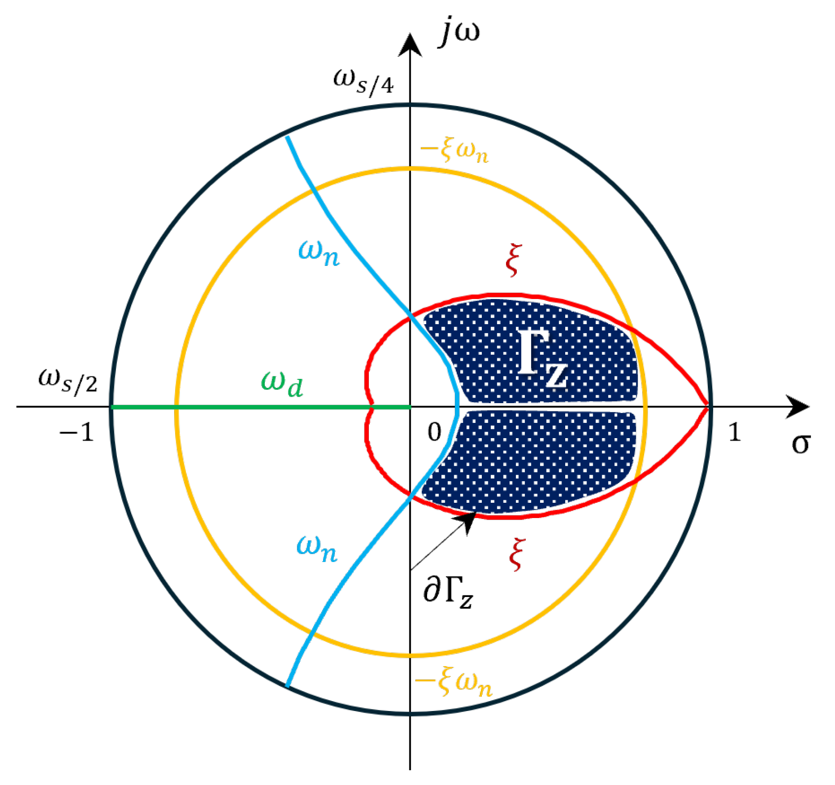
Figure 3.
Geometric interpretation of the magnitude of
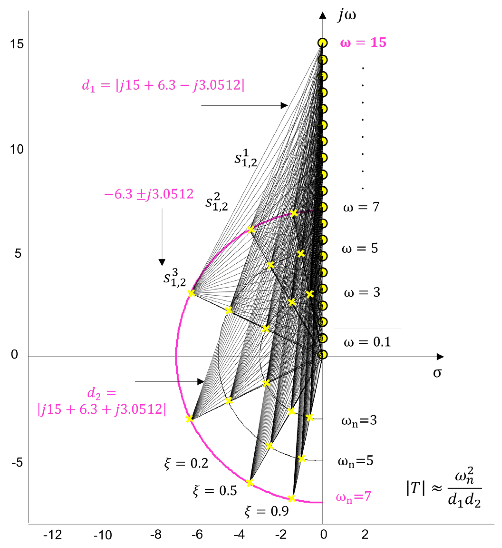
Figure 4.
and for .
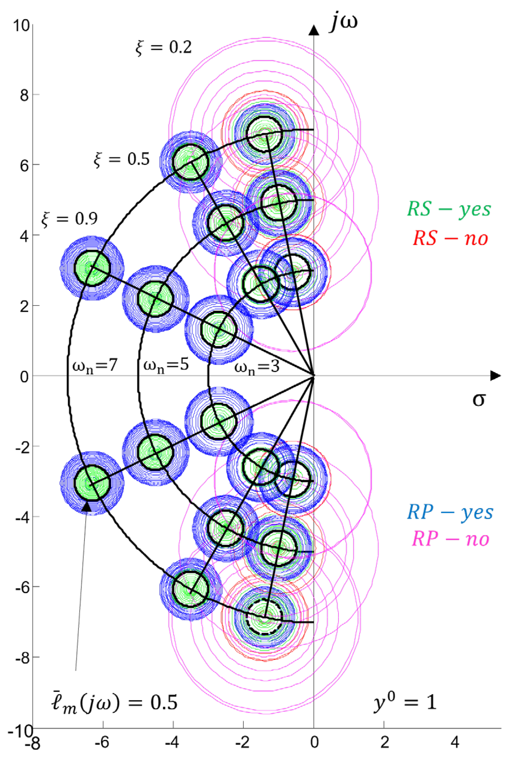
Figure 5.
and for
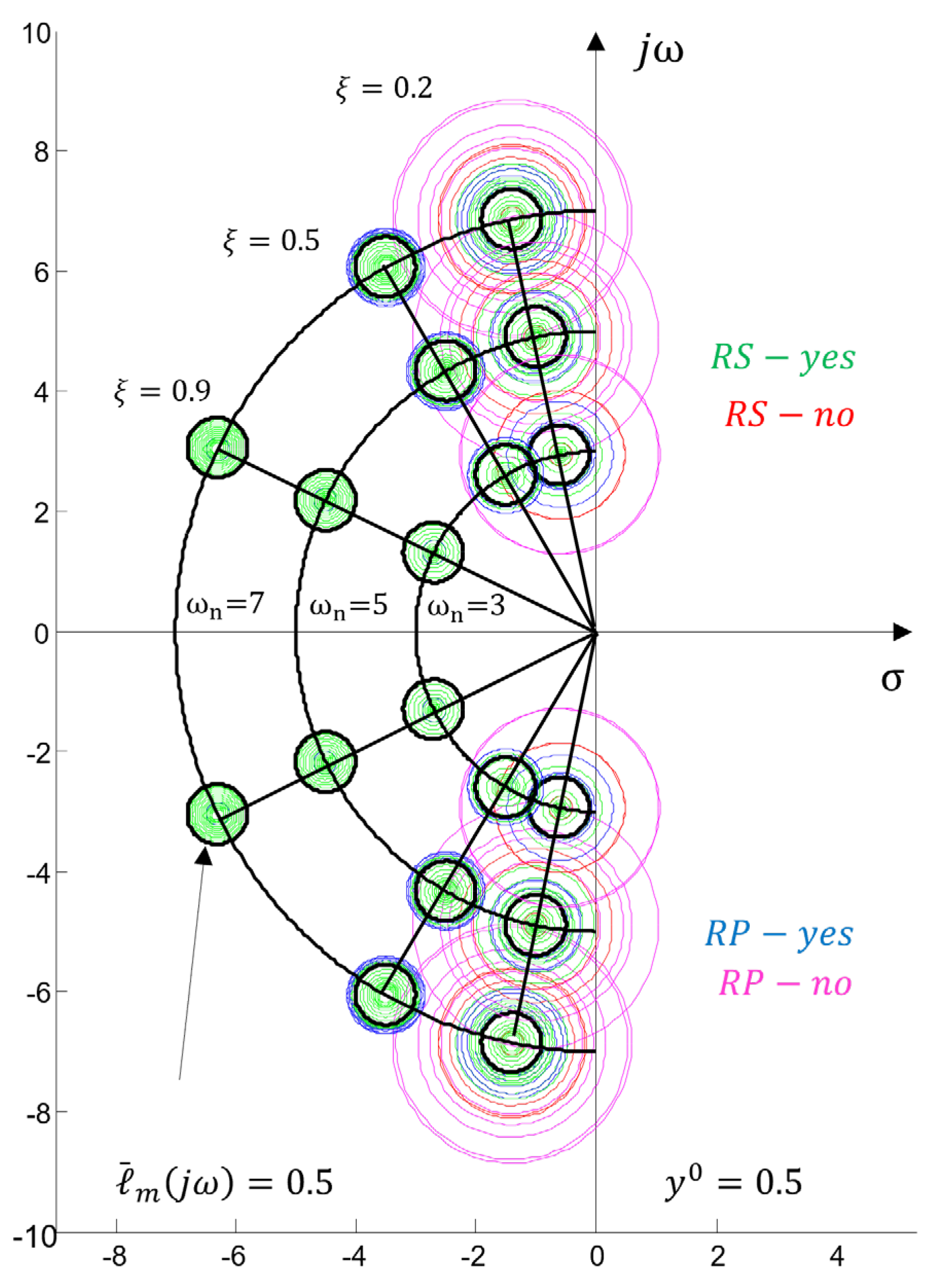
Figure 6.
and for .
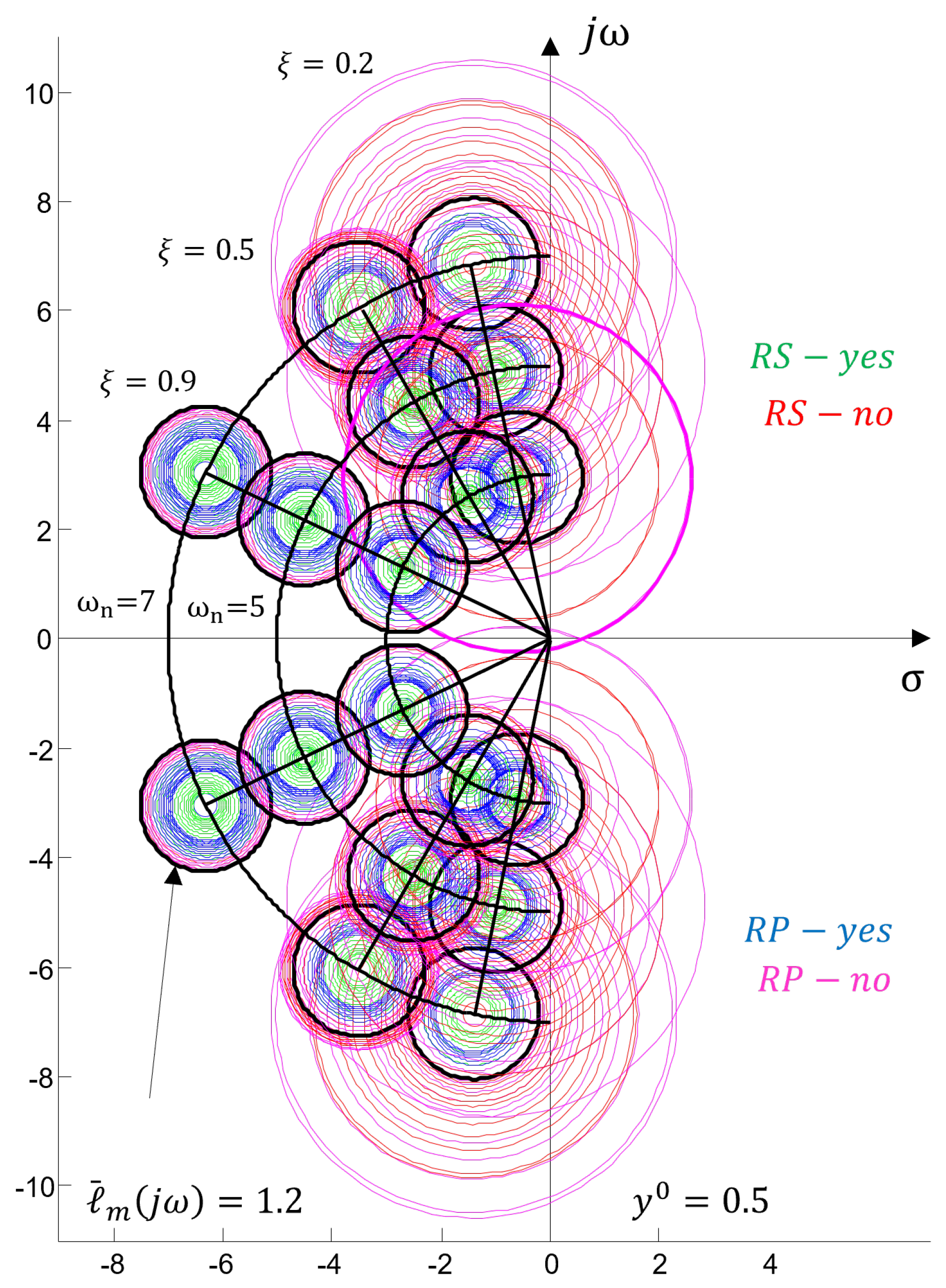
Figure 7.
and for
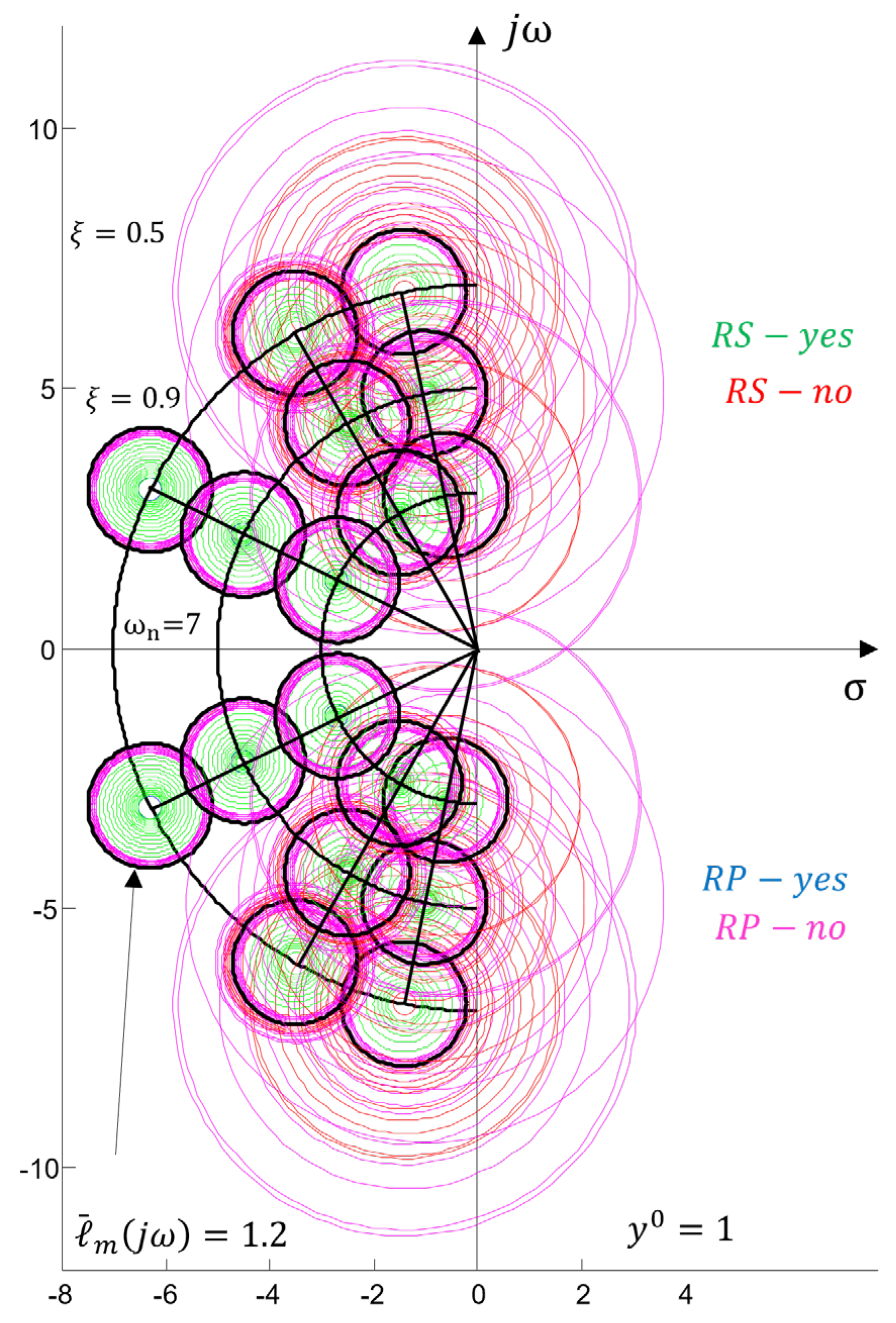
Figure 8.
for
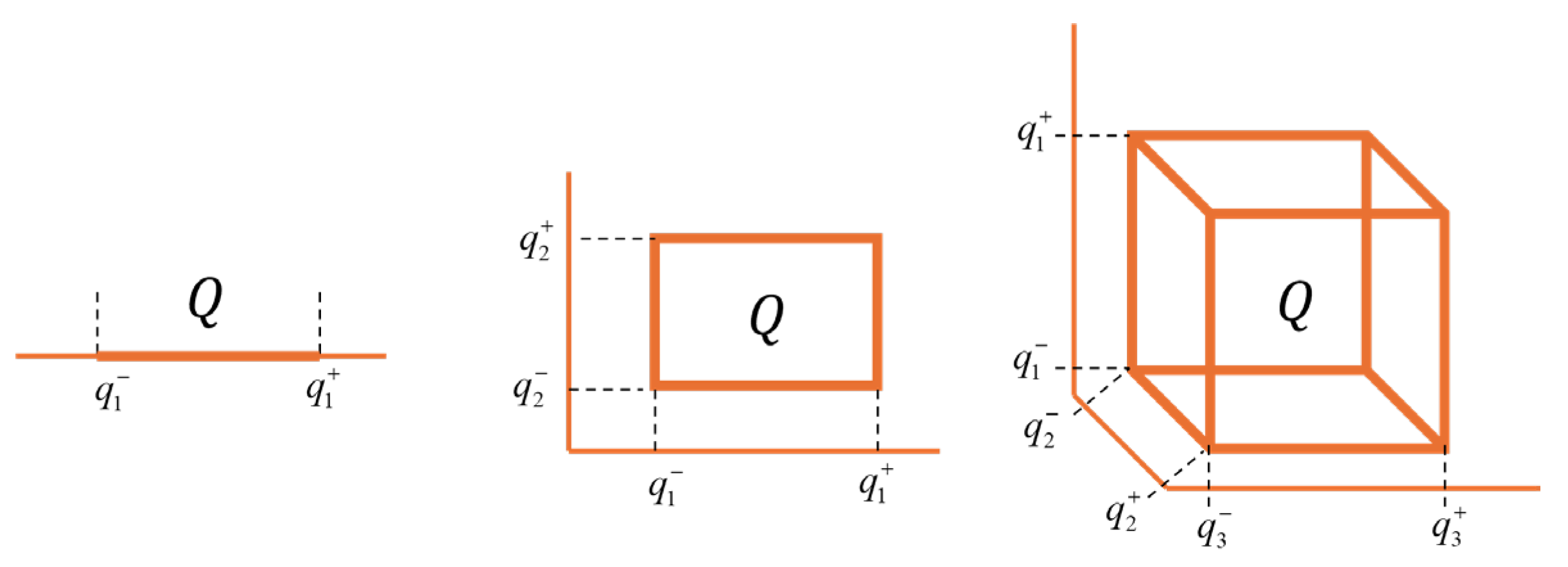
Figure 9.
, for .
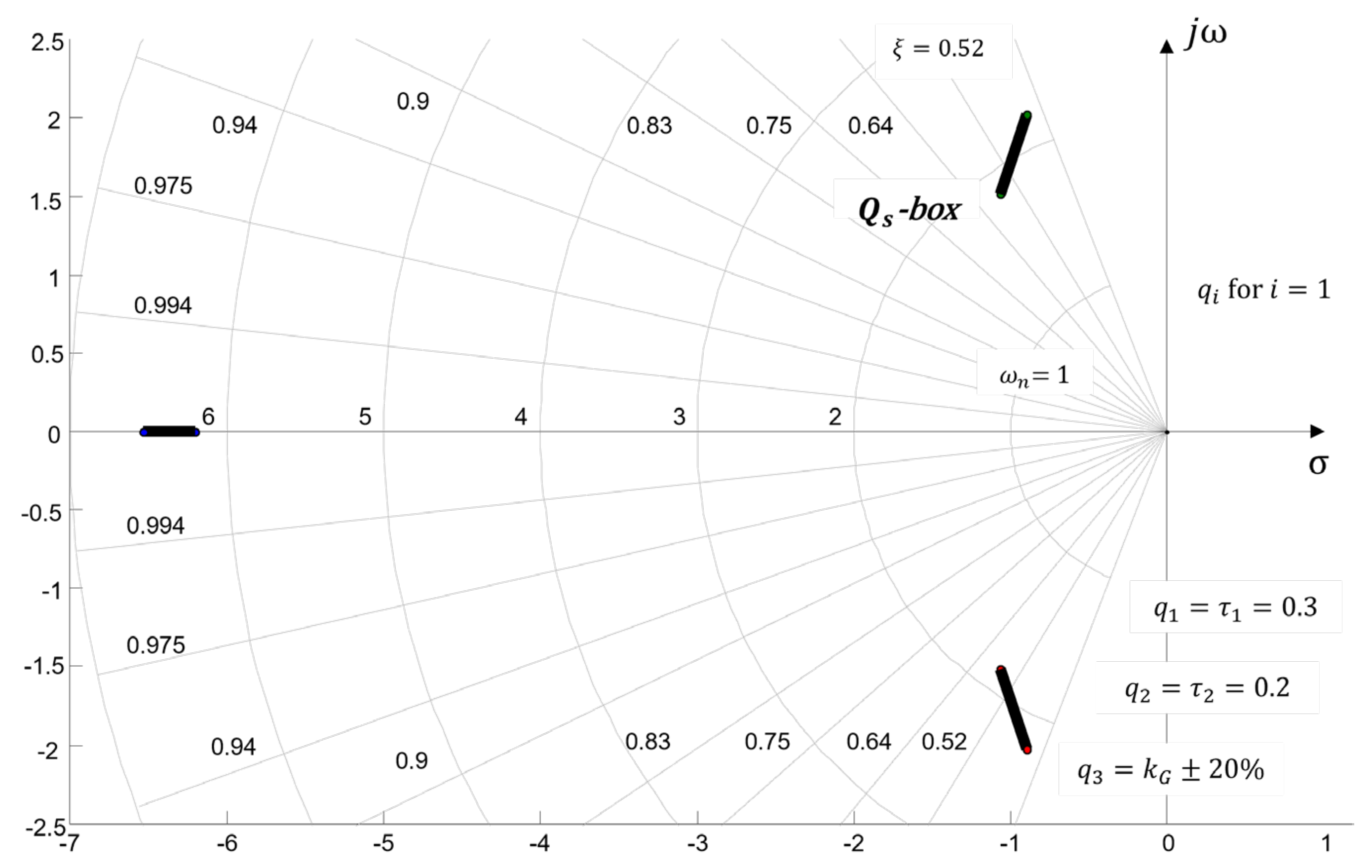
Figure 10.
, for
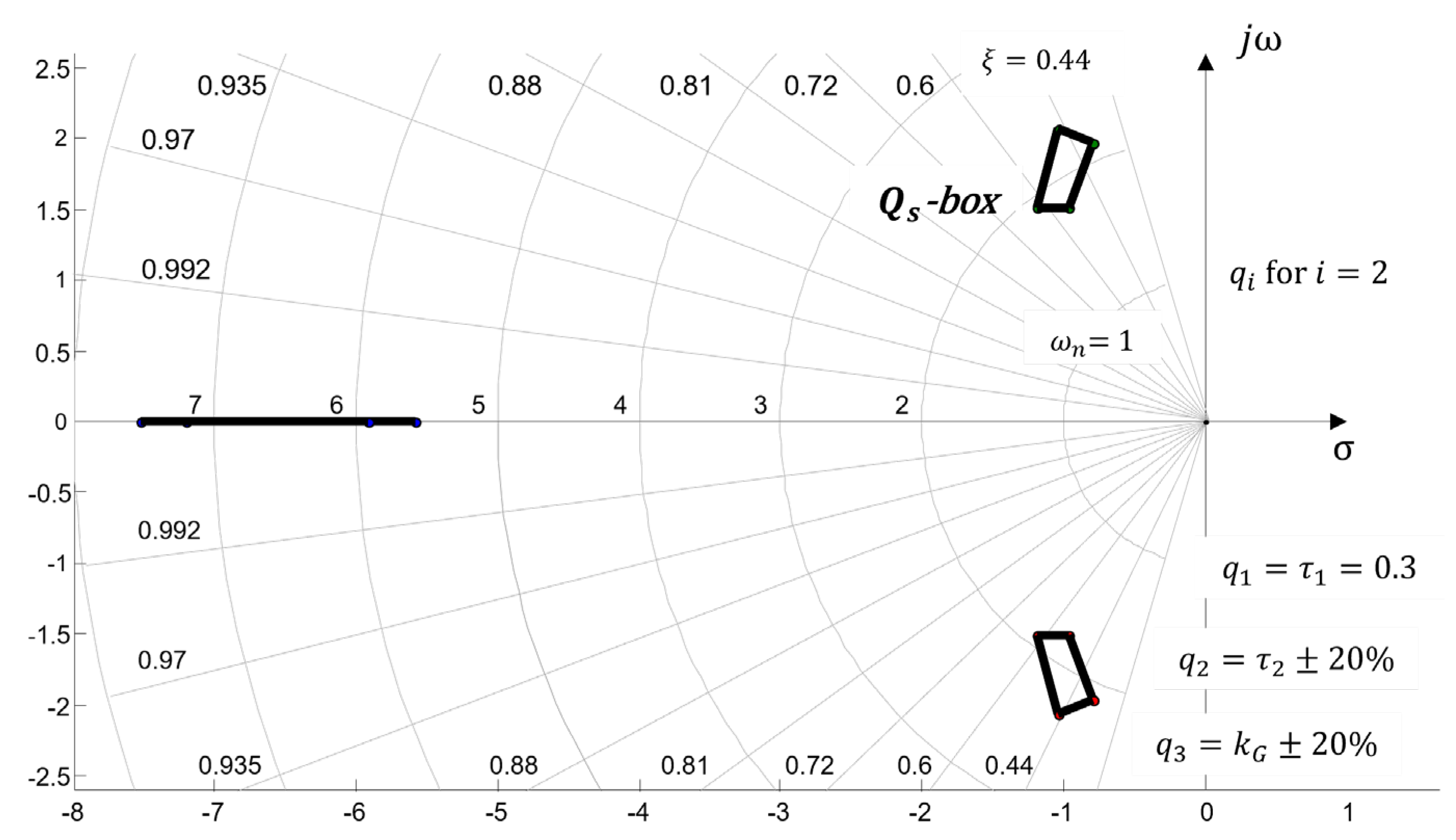
Figure 11.
for
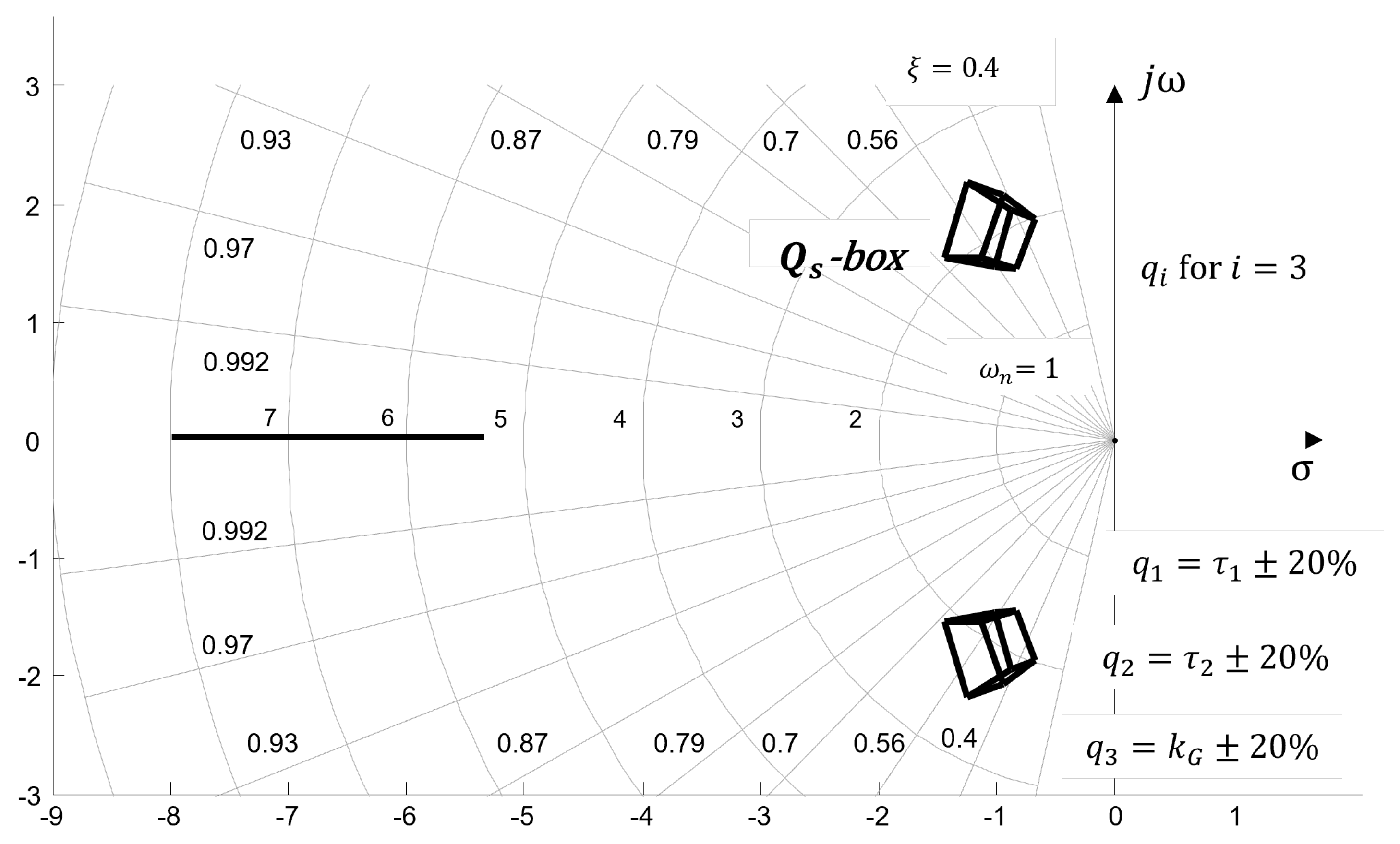
Figure 12.
Vertices of the
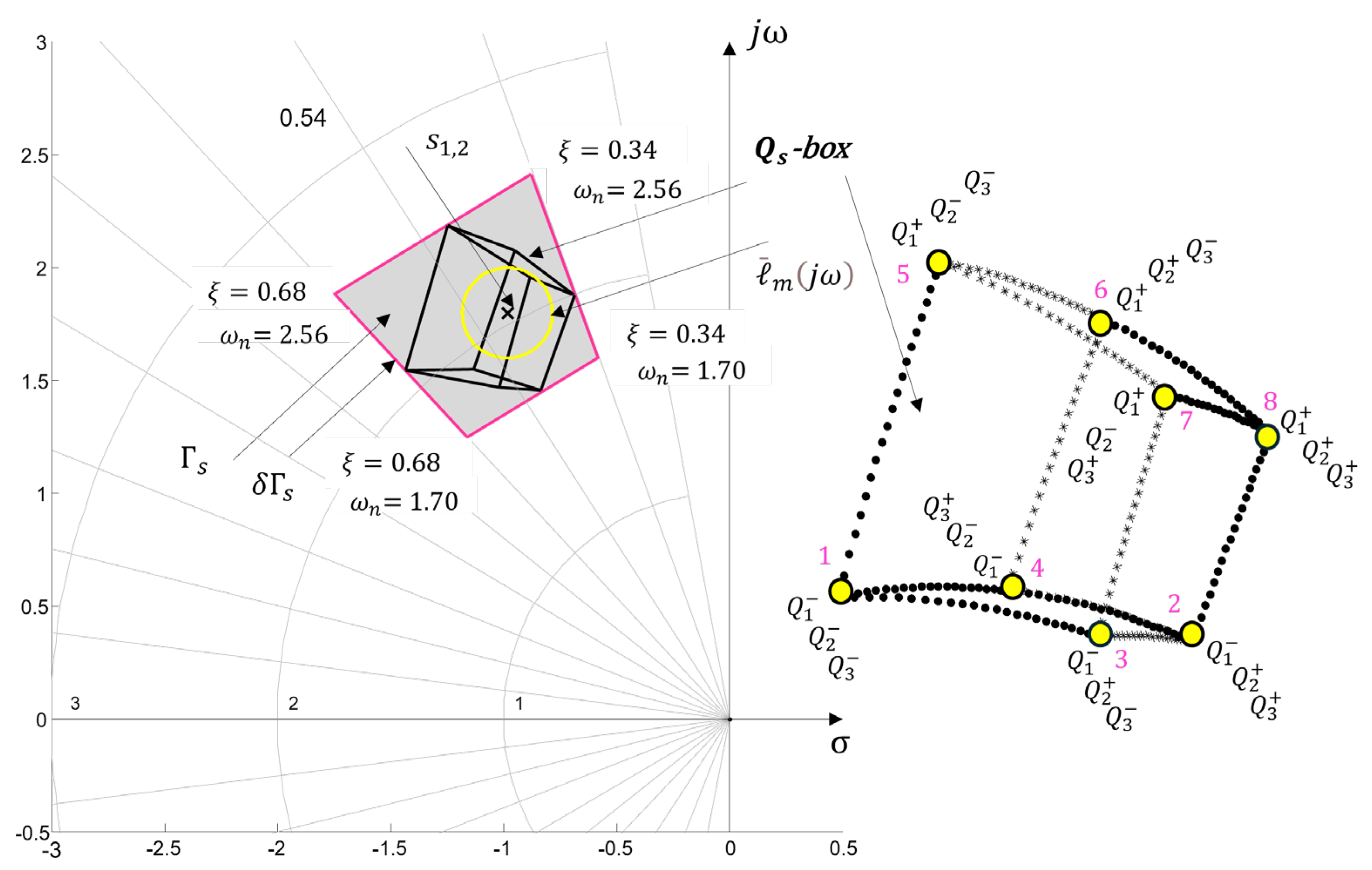
Figure 13.
, .
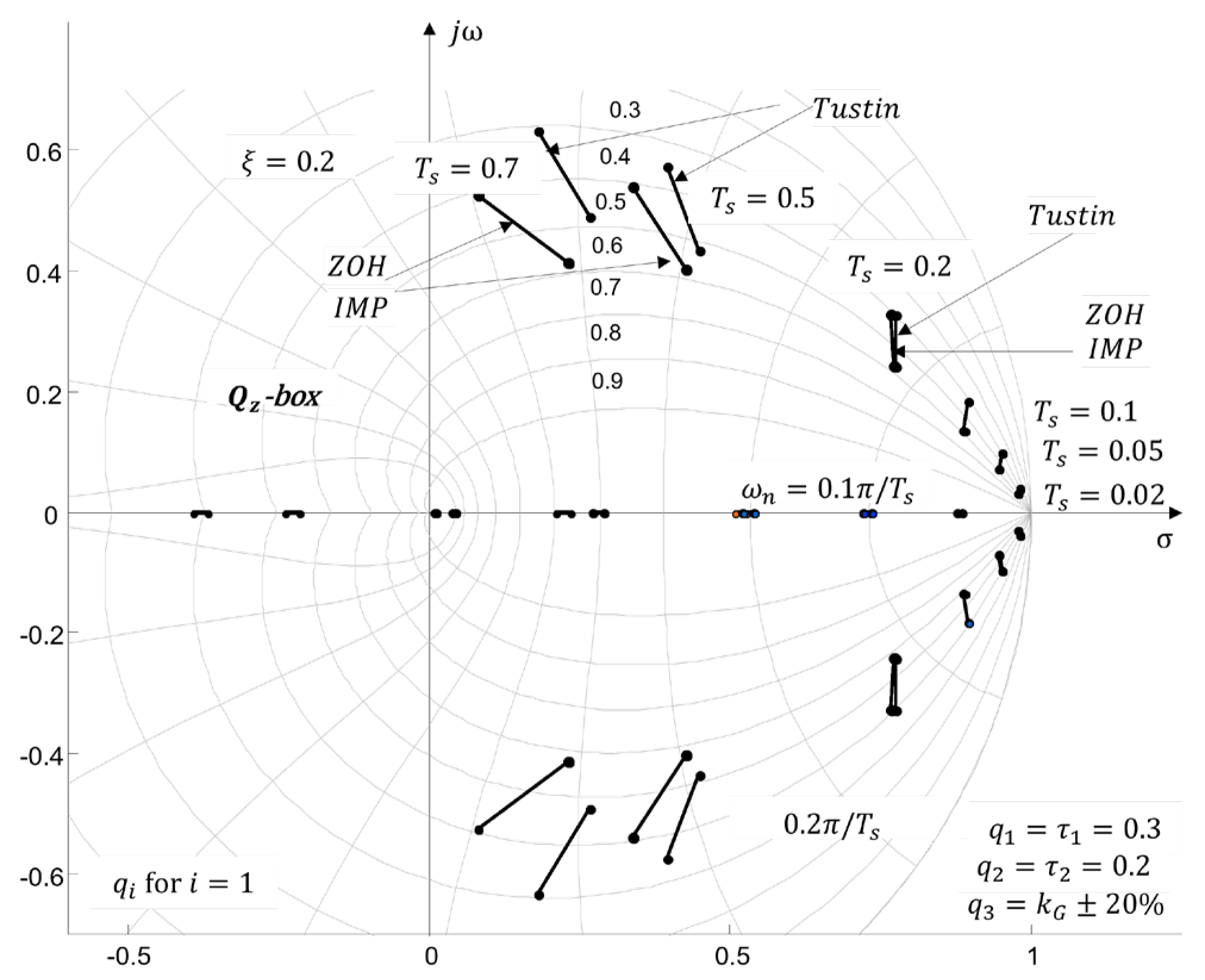
Figure 14.
, .
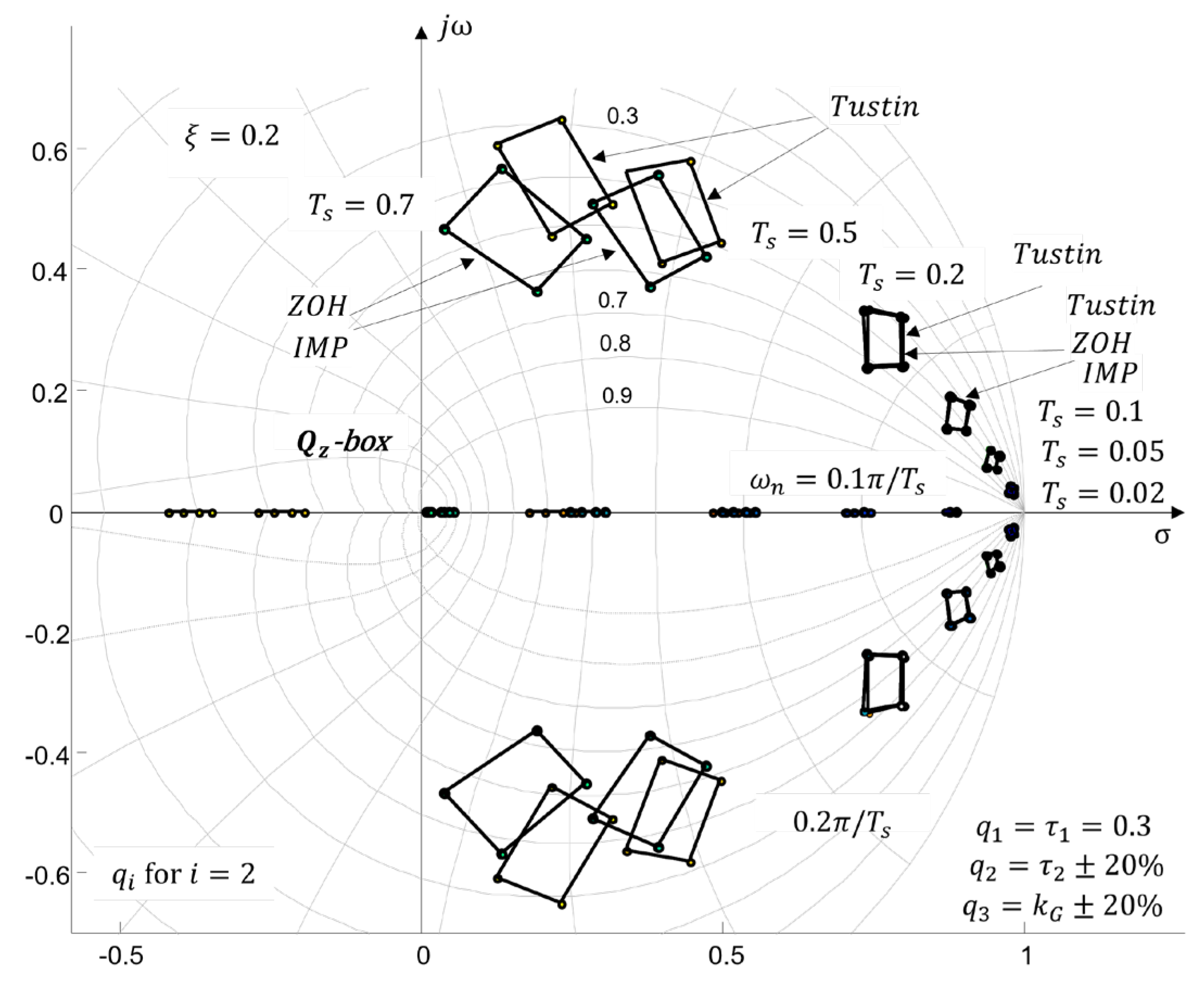
Figure 15.
, .
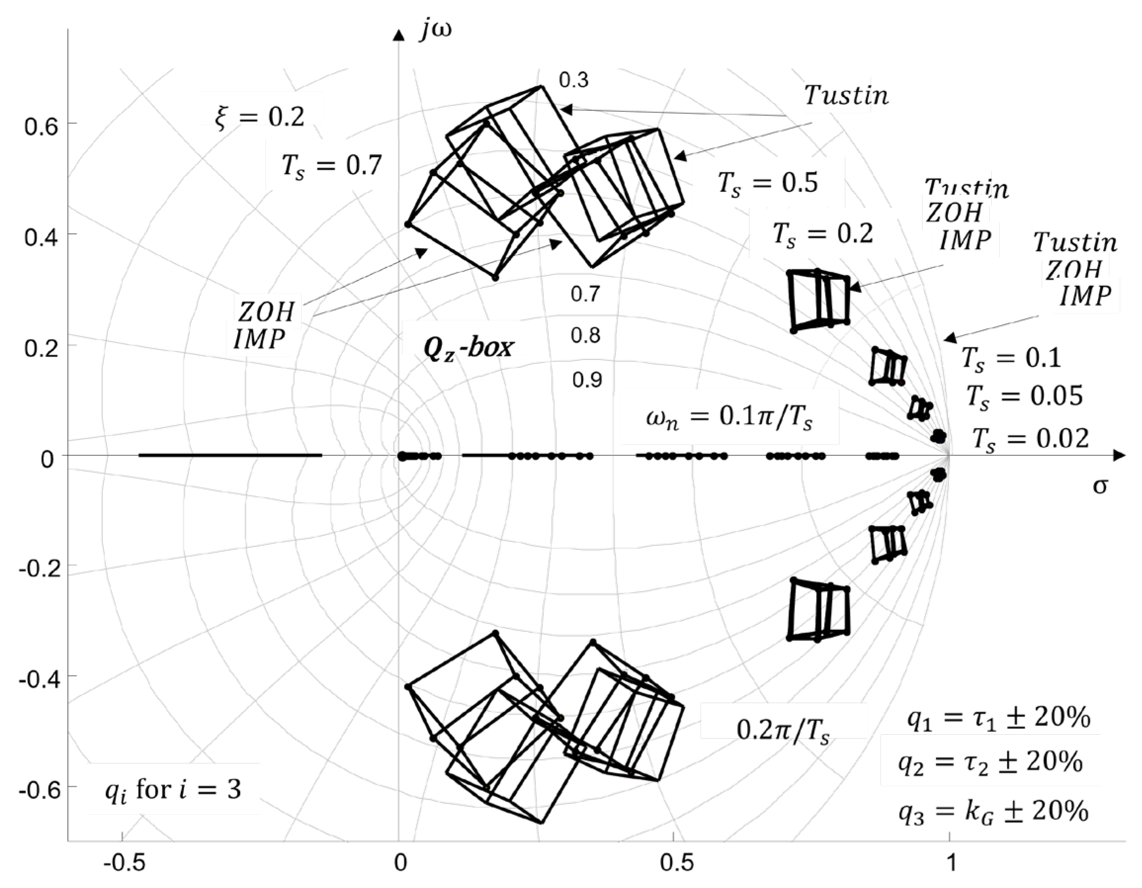
Figure 16.
Performance range
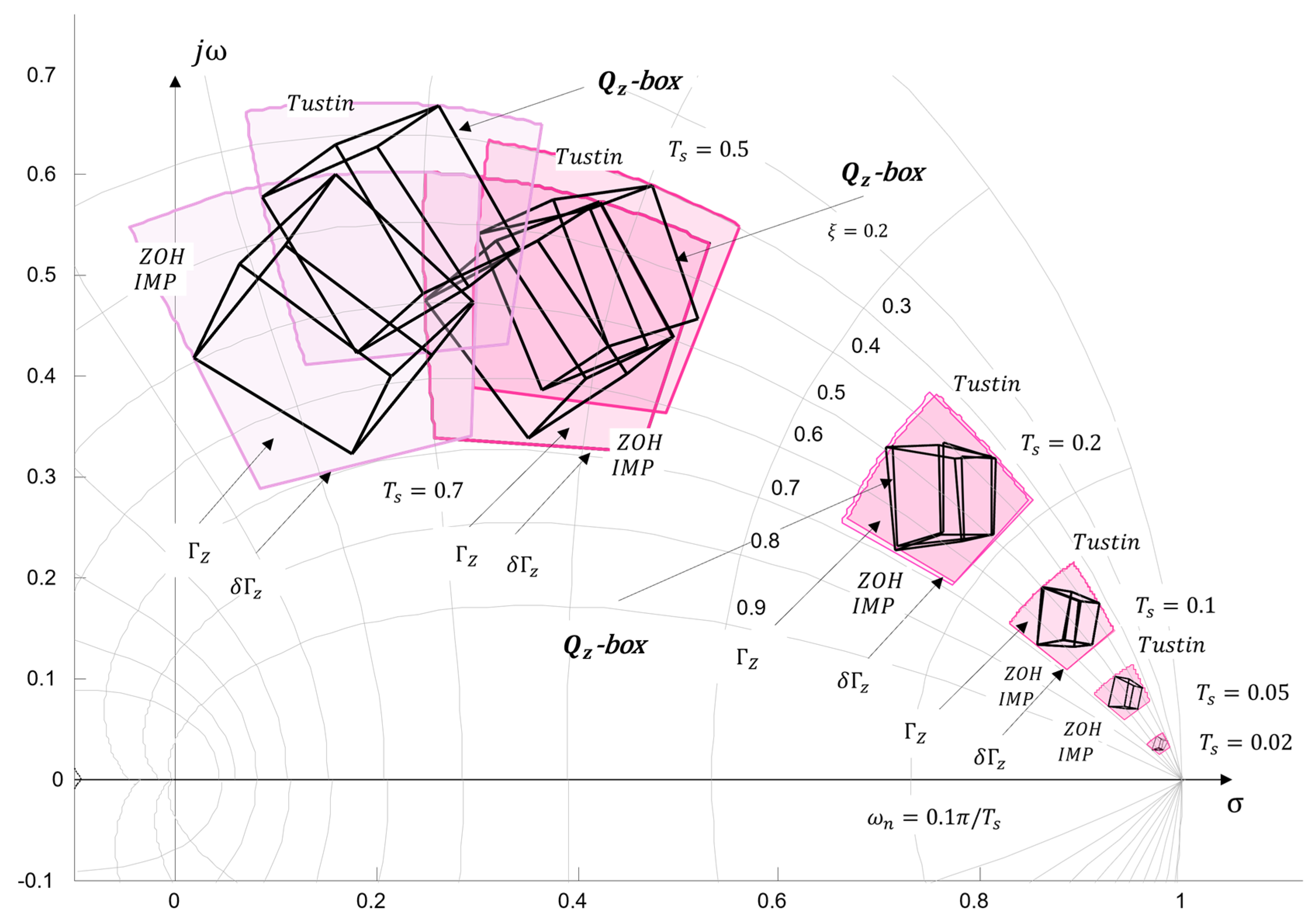
Figure 17.
Root locus of sampling time.

Figure 18.
for
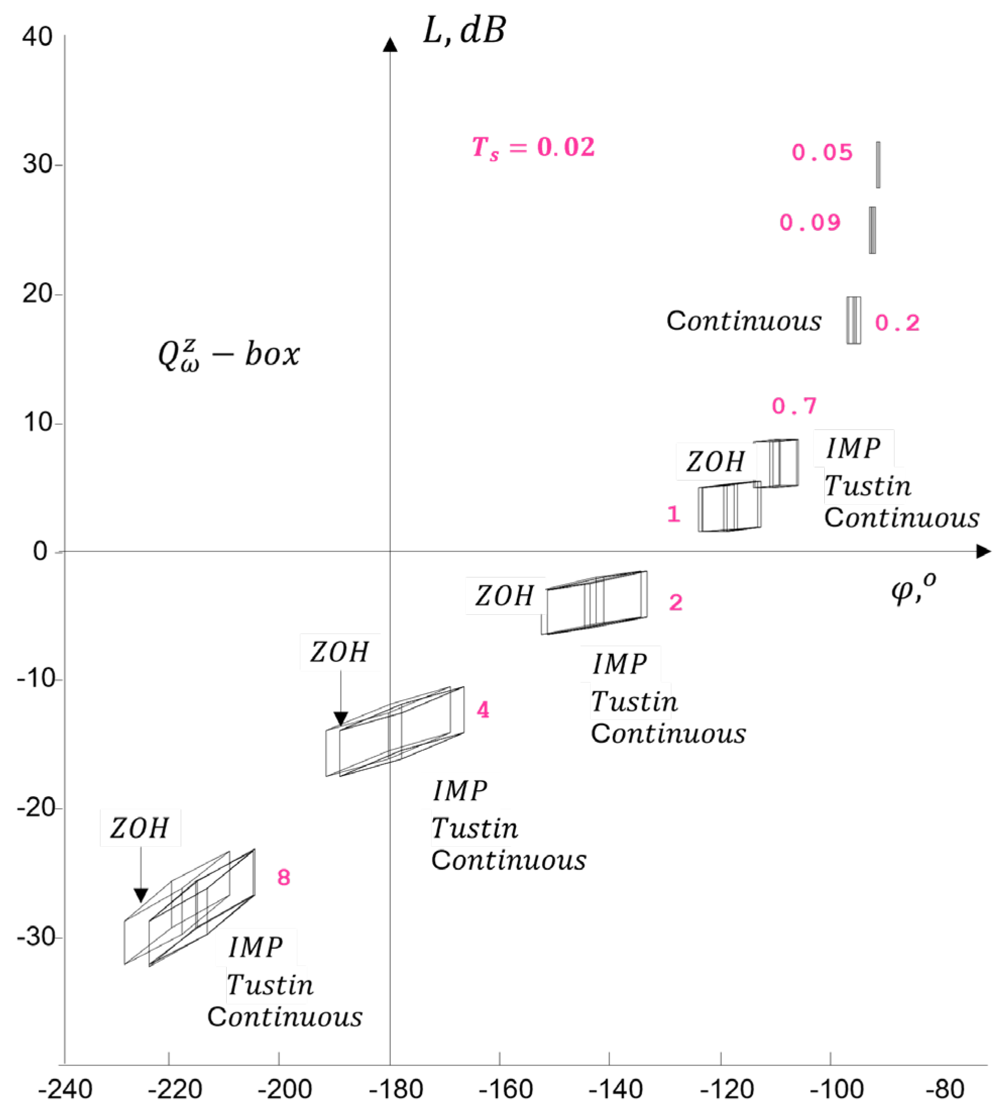
Figure 19.
for .
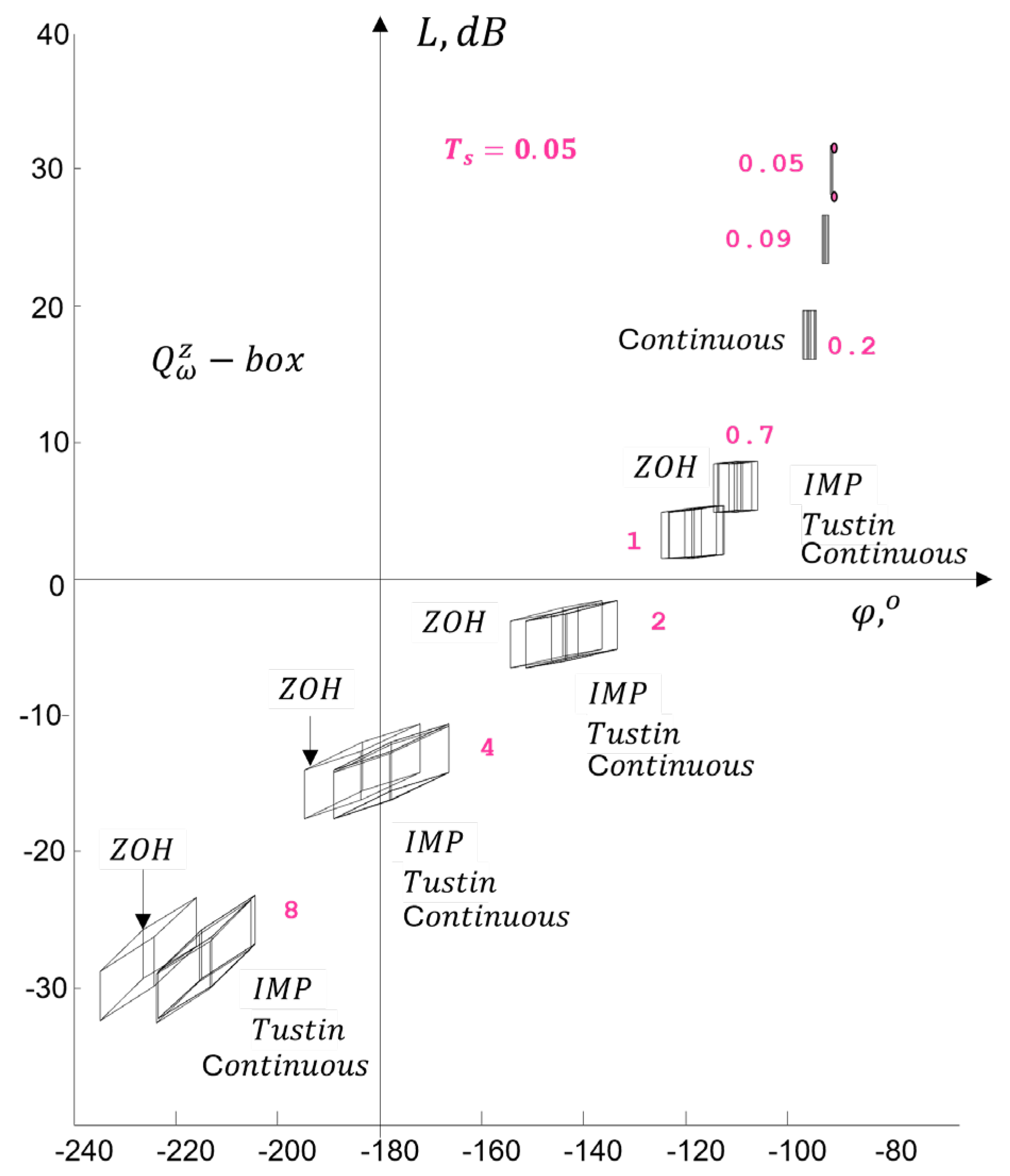
Figure 20.
for
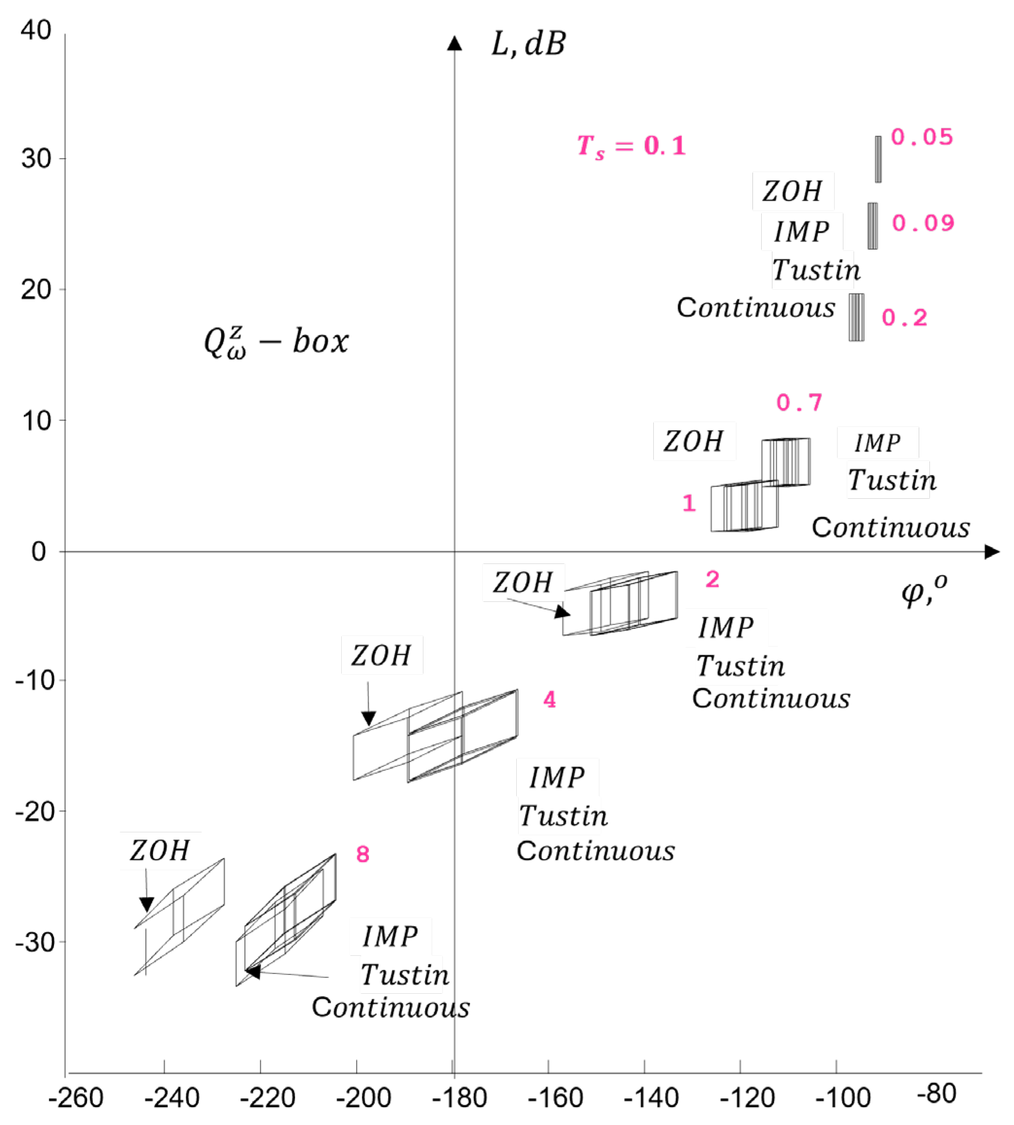
Figure 21.
for .
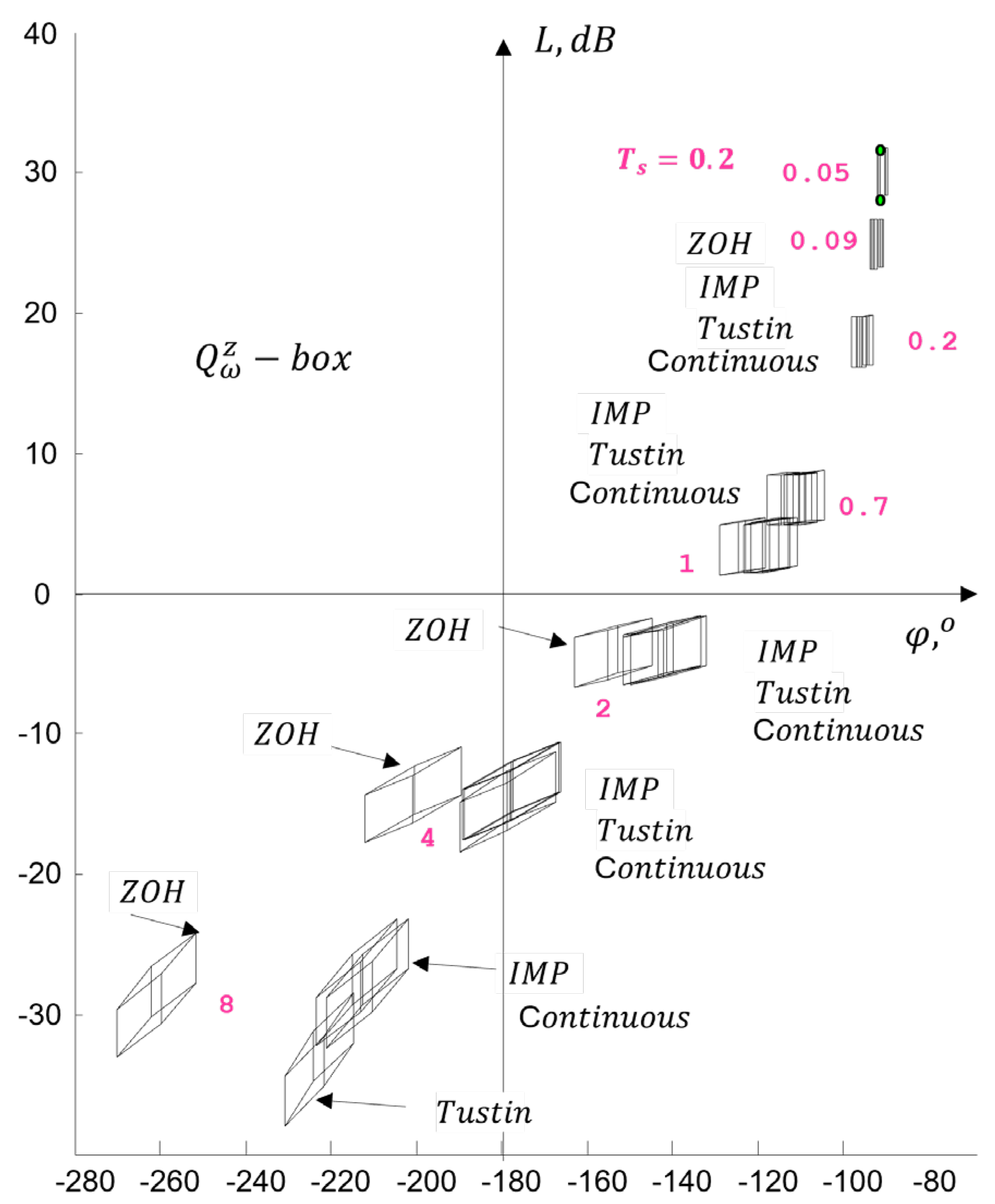
Figure 22.
for .
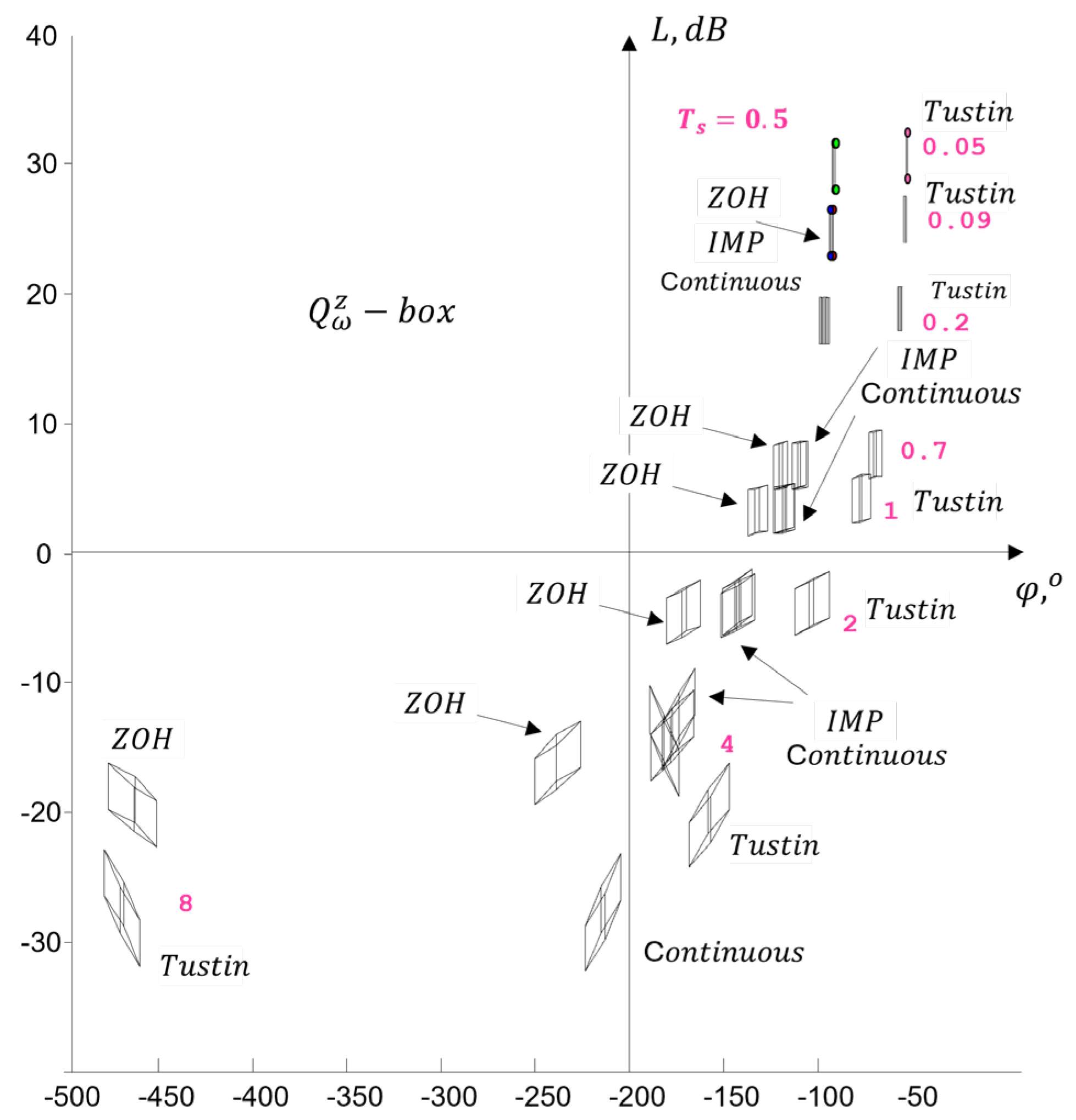
Figure 23.
for
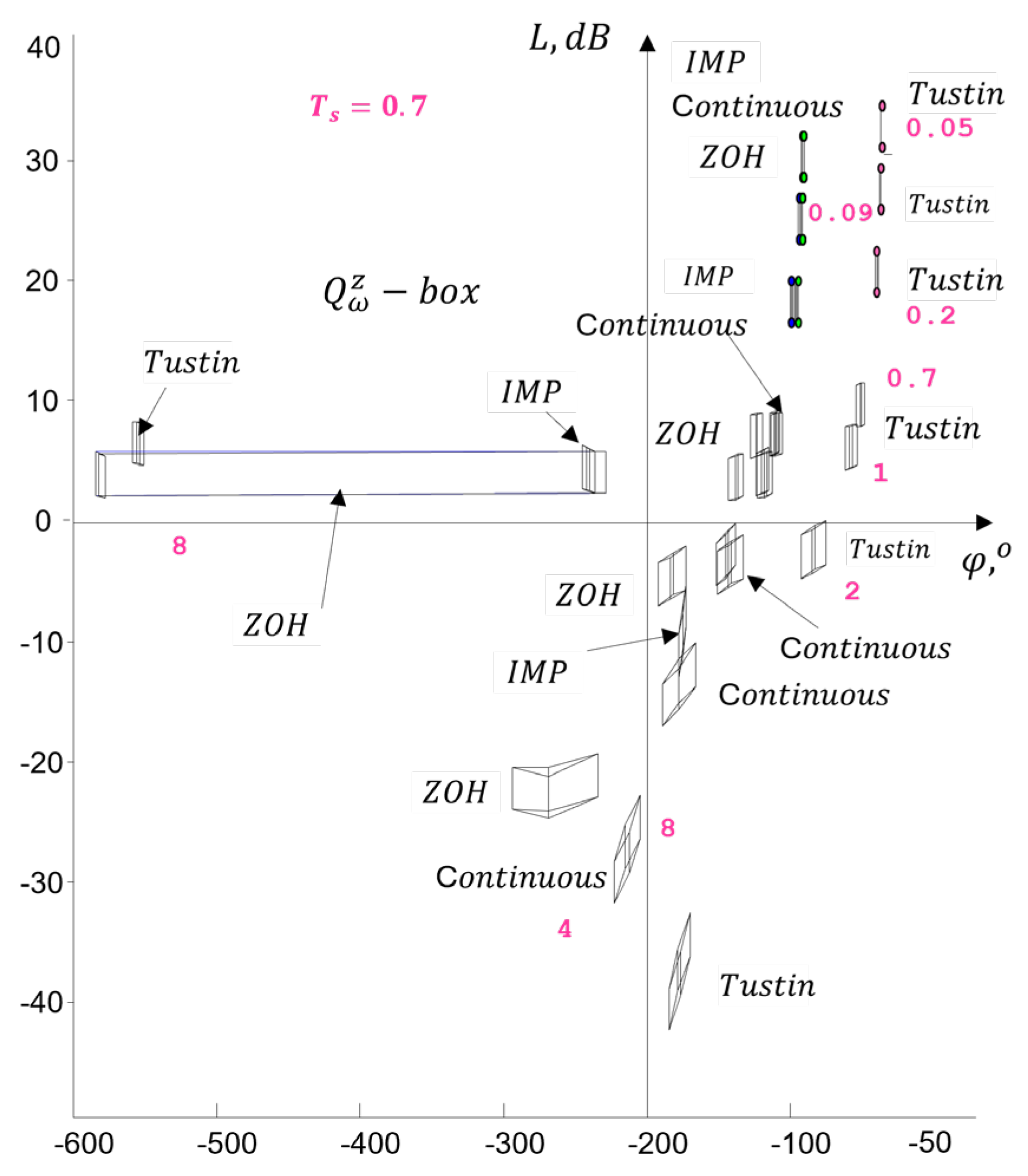
Figure 24.
and in Nyquist plot.
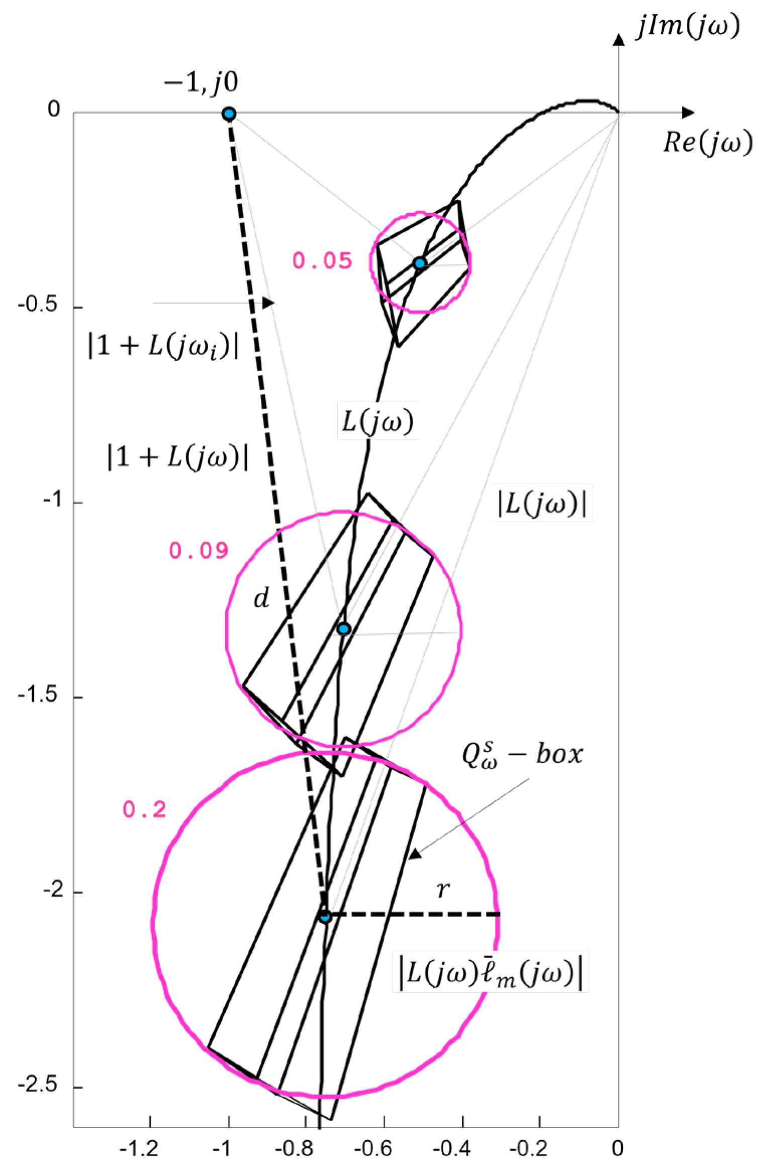
Figure 25.
Nichols plot representations.
Disclaimer/Publisher’s Note: The statements, opinions and data contained in all publications are solely those of the individual author(s) and contributor(s) and not of MDPI and/or the editor(s). MDPI and/or the editor(s) disclaim responsibility for any injury to people or property resulting from any ideas, methods, instructions or products referred to in the content. |
© 2025 by the authors. Licensee MDPI, Basel, Switzerland. This article is an open access article distributed under the terms and conditions of the Creative Commons Attribution (CC BY) license (http://creativecommons.org/licenses/by/4.0/).
Copyright: This open access article is published under a Creative Commons CC BY 4.0 license, which permit the free download, distribution, and reuse, provided that the author and preprint are cited in any reuse.


