
Submitted:
04 August 2025
Posted:
05 August 2025
You are already at the latest version
Abstract
Conventional unconditional random-field (URF) models were shown to neglect in‑situ monitoring data and thus to misrepresent real slope stability. To address this, a constrained random-field (CRF) generator was proposed, in which Fast Fourier Transform (FFT) filtering was coupled with co‑Kriging to assimilate site observations. A representative three‑bench slope was adopted, and the failure‑mode distribution and the statistics of the factor of safety (FoS) produced by the URF, the independent random field (IRF), and the CRF were examined across strata dip angles of 15°–75° and two cross‑correlation states ( = −0.2, 0). It was found that eliminating cross‑correlation decreased the mean FoS by 0.006, increased its standard deviation by 10.26 %, and raised the frequency of low‑FoS events from 7.49 % to 12.30 %. When field constraints were imposed through the CRF, the probability of through‑going failure was reduced by 12 %, the mean FoS was increased by 0.01, the standard deviation was reduced by 15.38 %, and low‑FoS events were suppressed to 2.30 %. The CRF framework was thus demonstrated to integrate stochastic analysis with field measurements, enabling more realistic reliability assessment and proactive risk management of slopes.

Keywords:
slope
; random field
; Fast Fourier Transform (FFT) filtering
; co-Kriging
; reliability analysis
1. Introduction
Rock and soil masses are natural materials with complex genesis. Owing to the multitude of structural planes and the highly uneven distributions of joints and fissures, critical mechanical parameters—such as cohesion and friction angle—exhibit marked spatial heterogeneity and multiscale variability [1,2,3,4]. Because limited field tests and sampling cannot fully capture this variability, substantial uncertainty surrounds assessments of overall slope stability [5,6]. For decades, engineers have largely relied on deterministic analyses, representing an entire study area with a single parameter set (or at most a few) to represent the entire area, thereby neglecting the spatial variability of material properties [7,8]. Such deterministic approaches fail to capture potential weak zones and the composite effects of alternating soft and hard strata that occur in real slopes, often under- or over-estimating safety risks and thereby compromising both the economy and reliability of design.
To overcome these deficiencies, numerical techniques such as the Random Finite Element Method (RFEM) [9,10] and the Random Finite Difference Method (RFDM) [11] have been widely adopted for complex slope-stability analyses. Anchored in random field theory, these methods characterize the spatial correlation, variability, and overall statistical distribution of geotechnical parameters within a probabilistic framework, thereby surmounting the limitations of deterministic approaches. Large-scale Monte Carlo simulations then produce reliability indicators—including failure probability, the distribution of safety factors, and the variability of potential slip surfaces—that furnish a more rigorous basis for risk evaluation and decision-making [12,13]. Most existing studies, however, still employ unconditional random fields (URFs) [10,11,13]; that is, they generate domain-wide random realizations using only prior statistics, without directly incorporating site investigation and testing data. This practice can result in “over-dispersion” or excessive conservatism, obscuring local strength characteristics and reducing the specificity and credibility of the reliability results.
Recent advances in geotechnical theory and information technology have underscored the pivotal role of field observations in producing scientifically sound reliability assessments [9,14]. Modern investigation techniques—such as borehole sampling, in-situ shear tests, and acoustic surveys—now yield reliable localized parameter data [15,16]. Accordingly, embedding these limited yet invaluable observations into random field models through conditional simulation has become a frontier research topic [17,18]. Appropriate conditioning calibrates the global random field, thereby improving both the accuracy and engineering relevance of slope-reliability analyses.
In response, this study proposes an integrated procedure for constructing conditional random fields (CRFs) by combining Fast Fourier Transform (FFT) filtering with co-Kriging interpolation. Using a representative three-bench slope case study, we conduct Monte Carlo simulations to compare slope failure patterns and safety-factor distributions for three models: the unconditional random field (URF), the independent random field (IRF), and the proposed CRF. These comparisons are carried out under varying bedding-dip angles and geotechnical parameter cross-correlation conditions. The specific objectives are to: (1) generate URFs via FFT filtering and examine how bedding-dip angle and parameter cross-correlation influence failure modes; (2) evaluate changes in stability results after removing cross-correlations (IRF); (3) construct CRFs with co-Kriging and quantify how field observations modify reliability outcomes; and (4) analyze the statistical distribution of safety factors, highlight differences among the random field models, and elucidate the technical advantages and practical value of CRFs in engineering reliability evaluations.
2. Method for Constructing CRFs
2.1. Generation of URFs via FFT Filtering
In geotechnical and rock-mechanics reliability analysis, both local spatial correlation and large-scale structural features of geomechanical parameters must be considered simultaneously [5,18,19]. An URF that satisfies a prescribed covariance function yields spatially correlated values at every point within the domain [1,20]. The FFT filtering technique provides an efficient means of generating such fields: by transforming the covariance function from the spatial domain into the frequency domain and filtering a white-noise field accordingly, one can rapidly construct a random field with the required correlation structure [21].
Before undertaking a reliability analysis, data from geological investigations, engineering experience, and laboratory tests must be integrated to derive the statistical characteristics of the rock–soil mass—namely, the mean, coefficient of variation, distribution type, cross-correlation coefficient, and correlation length [22,23]. These prior statistics underpin an accurate representation of the randomness and uncertainty inherent in geotechnical parameters. Because these parameters are non-negative and typically right-skewed, cohesion is commonly modeled with a log-normal distribution, whereas the friction angle is treated as normally distributed [17,24]. The relationship between their coefficients of variation and the logarithmic-space parameters is expressed as follows:
where and are, respectively, the standard deviation and the mean of the parameter in real space, while and represent the variance and the mean of the parameter in logarithmic space.
In view of the pronounced short-range correlation, long-range attenuation, and marked anisotropy of geotechnical parameters [25,26,27], an exponentially separable covariance function with explicit spatial structure is adopted. Its general form can be written as
where , , and are the correlation lengths of the parameter along the three principal directions, and , , and are the spatial lags in a rotated coordinate system that aligns with the dominant geological fabric. These rotated distances are given by:
where , , and are the rotation matrices that correspond to counter-clockwise rotations through the angles , , and about the , , and axes, respectively.
To impose the desired covariance structure in the frequency domain and thus create a random field with the prescribed statistics, the frequency-domain power spectrum is constructed as
where , , and are the discrete frequency indices that label grid points in the transformed domain; denotes the Hadamard (element-wise) product; is the white-noise spectrum, whose grid-point values are independent and follow ; and is the power spectral density derived from the Wiener–Khinchin theorem. and are the three-dimensional FFTs of the white-noise field and the covariance function , respectively. Their explicit forms are given by:
where , , and denote the numbers of grid points along the three principal axes; , , and are the spatial-domain indices; and is the imaginary unit.
A three-dimensional inverse FFT is then applied to the filtered spectrum , transforming the signal back into physical space and producing a realization of the random field that conforms to the prescribed covariance structure :
The filtered spatial field is finally standardized to produce a standard normal field , defined as
where and are the mean and standard deviation of , respectively.
To incorporate the spatial cross-correlation between the cohesion field and the friction-angle field, the correlated standard-normal fields are constructed as follows:
where and are the independent standard-normal fields produced in Eq. (9); is the cross-correlation coefficient between cohesion and friction angle; and denotes the standard-normal field for friction angle that is correlated with .
Given the marginal distribution assumptions for cohesion and friction angle, the correlated standard-normal fields obtained from Eq. (10) are mapped to random fields of mechanical parameters that respect the specified priors, namely,
where represents the cohesion random field that follows a log-normal distribution, whereas denotes the friction-angle field modeled as a spatially correlated truncated-normal distribution. The parameter is the empirically determined lower bound that guarantees remains non-negative across the domain. An illustrative realization of the fully spatially structured URFs generated by the FFT-filtering procedure is provided in Figure 1.
2.2. Construction of CRFs with the Co-Kriging Method
Co-Kriging is a multivariate geostatistical interpolation technique that exploits spatial cross-correlations between variables to obtain the statistically optimal estimate of multi-source data sets [28,29]. In this study, we refine the URFs with site-specific measurements through co-Kriging, thereby generating CRFs.
First, simulated values at the sampling locations are extracted from the URF and compared with their corresponding observations. The residuals of cohesion or friction angle, denoted , are calculated and adopted as conditioning data:
where is the measured cohesion (or friction angle) at sampling point , and is the corresponding value extracted from the URF.
Using these residual data , a residual field of the mechanical parameter is produced with the best linear unbiased estimator framework. Taking cohesion as an example, the estimated residual field at an unsampled location is expressed as
where and are the cohesion and friction-angle residuals located at and , respectively; and are the corresponding weight vectors. By imposing the unbiasedness condition and minimizing the estimation variance, these kriging weights are determined from the following system of linear equations:
where and are the auto-covariance matrices of the cohesion and friction-angle residuals (sizes and ); and are the cross-covariance matrices (sizes and ); , , , are column vectors of ones or zeros of length or , introduced to enforce the unbiasedness constraints; and are the Lagrange multipliers; and are the covariance vectors between the residuals at the sampled points and the target location for cohesion and friction angle, respectively (dimensions and ).
Assuming second-order stationarity, the auto--covariance function and cross-covariance function are written as
where is the lag distance—adjusted to the rotated coordinate system defined in Eq. (4); is the mean residual of cohesion or friction angle; is the number of sample pairs separated by lag .
Finally, the CRF is obtained by superposing the URF with the estimated residual field :
The CRF constructed herein simultaneously encapsulates the spatial variability of regionalized variables, their cross-correlations, and the constraints imposed by in-situ measurements, thereby furnishing a model that more faithfully represents in-service engineering conditions. Within a non-intrusive RFDM framework, the CRF parameters are mapped element-by-element onto the corresponding zones of a FLAC3D mesh. An iterative strength-reduction procedure is then executed to compute key response variables—most notably the safety factor of the slope and the maximum shear strain. These outputs form the basis for reliability assessment. The reliability index can be expressed mathematically as
where and are, respectively, the mean and standard deviation of the safety factor obtained from the RFDM simulations, and is the critical (target) safety factor. A comprehensive workflow of the entire procedure is presented in Figure 2.
3. Case Study
3.1. Model Configuration
To evaluate how the spatial variability of cohesion and friction angle—together with their cross-correlation—affects slope stability, we applied the proposed random-field framework to the slope model illustrated in Figure 3. The model measures 150 m (length) × 1 m (width) × 100 m (height). The engineered slope has a total height of 60 m and is divided into three benches, each 20 m high; the slope face dips at 60°, and every bench platform is 20 m wide.
Boundary conditions are specified as follows: normal displacements are constrained on the lateral faces, all degrees of freedom are fixed at the base, and the upper surface is free, being loaded only by self-weight in the vertical (-z) direction. The finite-difference mesh primarily comprises 1 m hexahedral zones, with a small number of tetrahedral zones of comparable size near geometric irregularities, giving a total of 10,751 zones. The prior statistical parameters adopted for the rock–soil mass are summarized in Table 1.
In the model, six investigation points are predefined and arranged in two boreholes—one on the uppermost bench and the other on the lowest bench. Each borehole contains three sampling points spaced 6 m apart. To quantify how these pointwise constraints affect slope stability, we first perform Monte Carlo simulations with URFs and IRFs generated via FFT filtering; we then incorporate the co-Kriging scheme to create CRFs. Finally, the failure patterns and safety factors obtained under the three random-field scenarios are compared.
3.2. Slope-Stability Analysis with URFs
Building on the model introduced in Section 3.1, we generate spatially complete random fields of the mechanical parameters in the frequency domain. A series of Monte Carlo experiments—with diverse combinations of geological orientation (bedding dip) and parameter cross-correlation—are carried out to systematically examine how spatial anisotropy and inter-parameter dependence influence failure mechanisms and safety factors.
Correlation lengths are set to 20 m in the x direction and 3 m in the z direction. To emulate the typical mismatch whereby local zones of low cohesion coincide with relatively high friction angles, the cross-correlation coefficient between the two parameters is fixed at −0.2. Five bedding-dip angles—15°, 30°, 45°, 60°, and 75°—are considered to capture anisotropy controlled by stratification; the resulting anisotropic parameter fields are illustrated in Figure 4.
For each bedding-dip angle, 200 independent URFs were generated, yielding a total of 1,000 realizations. After mapping these parameter fields to the numerical-model zones, the slope was driven to failure with the strength-reduction method (SRM), and the plastic-shear-strain distribution was used to delineate potential failure zones. As illustrated in Figure 5, the large result set was systematically classified according to the spatial relationship between the through-going plastic zones and the bench structure, enabling cross-comparison among dip angles. Nine representative failure modes (M1–M9) were ultimately distilled: Specifically, M1 is an overall failure penetrating all three benches; M2–M4 are local failures of the upper, middle, and lower single benches, respectively; M5–M7 are two-bench combined failures; M8 is a two-bench failure penetrating the upper and middle benches; and M9 corresponds to three benches failing independently.
To quantify how the bedding-dip angle governs both the distribution of failure modes and the slope-safety margin, the Monte Carlo results for each dip setting were post-processed to obtain the percentage share of every failure mode and the mean safety factor. The aggregate statistics for all 1,000 realizations serve as a benchmark. The compiled results are displayed in Figure 6.
Figure 6a shows that slope failures are dominated by either global, through-going collapse (M1) or single-bench, localized failures (M2–M4), which together account for more than 80 % of all realizations; complex composite modes are comparatively rare. The share of global failure (M1) follows a U-shaped trend with respect to bedding-dip angle, being high at shallow (15°) and steep (75°) dips but reaching its minimum (42 %) at 45°. In contrast, the lower-bench failure mode (M4) peaks at a dip of 45 % (15.5 %).
Figure 6b indicates that the safety factor (FoS) remains within a narrow band of 1.113 – 1.219 across all dip angles. The FoS for global failure (M1) is consistently lower than that for upper- (M2) and middle-bench (M3) failures, yet similar to that for lower-bench failure (M4). This pattern suggests that localized shear slips generally require a larger reduction factor to coalesce, whereas the lower bench—owing to stress concentration—tends to fail first and can trigger a transition from localized to global collapse (Figure 7). Moreover, the FoS associated with the global mode (M1) increases with bedding dip, implying that gently dipping strata oriented subparallel to the 60° bench face are more susceptible to slope instability.
3.3. Slope-Stability Analysis with IRFs
To isolate and quantify the influence of cohesion–friction-angle cross-correlation on slope behavior, we first examined the –0.2 case and then generated a second suite of random fields in which the cross-correlation coefficient was deliberately set to zero. In this IRF, the spatial fluctuations of cohesion and internal friction angle are entirely decoupled, eliminating the “weak-versus-strong” compensatory effect and enabling a clearer assessment of how correlation shapes failure patterns and safety factors. Figure 8 presents representative realizations of the mechanical-parameter fields produced under both correlation settings.
Figure 8 highlights how altering the cross-correlation coefficient markedly changes the heterogeneity of the mechanical-parameter fields. When the coefficient is –0.2, zones of low cohesion are typically offset by locally high friction angles, illustrating a “weak-strong” compensatory effect.
For the IRF analysis, 200 statistically independent realizations were generated for each of the five bedding-dip angles, yielding 1,000 simulations in total. All other model attributes—marginal statistics, correlation lengths, mesh, and boundary conditions—were identical to those described in Section 3.2. The results were post-processed to determine, for each dip angle, the proportion of the various failure modes and the mean safety factor (Figure 9a,b). Comparison matrices that summarize the differences relative to the URF case are presented in Figure 9c,d.
When the cross-correlation between cohesion and friction angle is removed, weak zones are characterized by simultaneously low values of both parameters, which reduces the local shear strength and renders the slope more susceptible to localized instability. As illustrated in Figure 9(c), the failure-mode distribution in the IRF undergoes a pronounced redistribution. In the absence of the compensatory effect, the proportions of the upper-bench (M2) and lower-bench (M4) localized-failure modes increase markedly—to 1.20 and 1.10 times those observed in the URF case, respectively. Because both M8 and M3 involve slip-out of the middle bench, the risk of failure in that bench also rises. By contrast, the frequency of the global through-going mode (M1) at steep bedding dips (60°–75°) decreases to 0.77 times that of the URF. Figure 9(d) further shows that the mean safety factor of the IRF declines overall, yet the reduction is modest (less than 2 %). These results indicate that, relative to the slight change in safety factor, the loss of parameter correlation exerts a far more significant influence on the distribution of failure modes.
3.4. Slope-stability analysis with CRFs
The preceding URF and IRF studies underscored how the spatial correlation structure of cohesion and friction angle shapes failure mechanisms. In practice, however, the sparse site-investigation data available for most projects are seldom exploited in traditional random-field frameworks. To make reliability assessments more targeted and credible, CRFs approach was adopted: the URFs generated in Section 3.2 were jointly conditioned on the six in-situ measurements by means of co-Kriging, thereby quantifying how field observations modify the reliability outcome. Figure 10 presents the resulting mechanical-parameter CRFs with a cohesion–friction-angle cross-correlation coefficient of −0.2.
For each of the five bedding-dip angles considered—15°, 30°, 45°, 60°, and 75°—200 realizations of the CRF with a cross-correlation coefficient of −0.2 were generated, yielding a total of 1,000 realizations. Under otherwise identical modeling conditions, the simulation outcomes were post-processed to obtain the proportion of each failure mode and the mean safety factor for every dip angle (Figure 11a,b). To highlight the influence of conditioning, the corresponding statistics were further organized into comparison matrices (Figure 11c,d).
Figure 11(c) shows that the high-strength constraint at the mid-depth sampling point of Borehole 2 suppresses the occurrence frequency of the M1 failure mode to 0.88 times its baseline value, whereas the low strength measured at the upper sampling point of Borehole 1 promotes a 1.21-fold increase in the proportion of M2. Notably, the “low-over-high” vertical strength profile observed in Borehole 2 imparts a marked dip-angle dependence to M4. This constraint narrows the extension angle available to potential slip surfaces and favors their penetration through the steeply dipping strata; consequently, the share of M4 rises sharply at steep dips (60° and 75°) but declines at gentle dips (15° and 30°). The corresponding increases in the mean factor of safety for M4 under gentle dips—1.038 and 1.023 times, respectively, as plotted in Figure 11(d)—corroborate this trend.
Moreover, the proportion of M1 still follows a “U-shaped” distribution. From a mechanical standpoint, both gently and steeply dipping strata easily develop local step-like rock bridges that delay instability. During the strength-reduction analysis, an incipient slip surface that cannot breach these local steps eventually propagates along zones of concentrated shear stress, leading to overall failure.
To further quantify the effects of dip angle and the spatial random-field model on slope stability, the distribution maps of the factor of safety are provided in Figure 12.
Figure 12 systematically displays the kernel-density curves of the FoS obtained from three spatial random-field models— URF, IRF, and CRF—evaluated at five bedding-dip angles, together with their key statistics ( and ). For direct comparison, Figure 12(d) superimposes the aggregate histograms of the three models and their corresponding Gaussian fits.
The results reveal that both URF and IRF distributions are mildly right-skewed, with the IRF exhibiting a noticeably heavier right tail, whereas the CRF curve is nearly symmetric and shows well-converged tails. Relative to the URF baseline, the CRF distribution shifts rightward by 0.010 and becomes narrower, while the IRF shifts leftward by 0.006 and widens; the URF lies between these two extremes. These shifts indicate that, once the negative cross-correlation between cohesion and friction angle is removed in the IRF, the “weak–weak” co-location mechanism of mechanical parameters not only lowers the mean FoS but also enlarges its dispersion ( rises by 10.26 %). Conversely, incorporating field observations in the CRF effectively contracts the predictive uncertainty ( declines by 15.38 %), an effect that is most pronounced at low dip angles where local weakness exerts stronger control.
Assuming a short service life for the slope and negligible consequences upon failure, a critical FoS of 1.1 is adopted. Based on the fitted distributions, the calculated failure probabilities for the URF, IRF, and CRF are 7.49 %, 12.30 %, and 2.30 %, respectively, yielding reliability indices of 1.452, 1.152, and 2.011. These figures substantiate the substantial improvement in slope reliability achieved by incorporating observation-based constraints.
4. Discussion
This study systematically compares slope stability outcomes using three different random field descriptions: URF, IRF, and CRF. The comparison highlights the strong influence of spatial variability, cross-correlation, and fields measurements on both failure mechanisms and factor-of-safety (FoS) statistics.
- (1)
- Failure mechanisms. Incorporating field observations substantially changes the evolution of the incipient slip surface. In the CRF model the probability of through-going failure (Mode M1) is markedly lower than in the URF, whereas modes characterised by local sliding or multi-step combinations (e.g. M2, M8) become much more frequent. Borehole data locally update the material strength, which in turn inhibits the formation of continuous low-strength bands and mitigates the risk of a large, penetrating slip surface. At the same time, the revealed weak zones trigger shear instability in the upper benches. This behaviour is consistent with the shallow, small-scale failures commonly observed in practice.
- (2)
- Statistical characteristics of the FoS. The CRF increases the mean FoS slightly (≈ 0.01) while reducing its variance by roughly 15 %, yielding a markedly more concentrated distribution with thinner tails. This convergence is most pronounced at intermediate bedding dips of 15°–45°, underscoring the decisive role of observation constraints in controlling local weakening zones and illustrating a robustness effect arising from the inclusion of field information together with parameter cross-correlation..
- (3)
- Consistency of input parameter fields (Figure 13). Goodness-of-fit tests show that the generated cohesion field (log-normal) and friction-angle field (truncated normal) reproduce the prescribed marginal distributions well (mean Kolmogorov–Smirnov statistic D < 0.035). The sample mean of the target cross-correlation coefficient (ρ = −0.2) deviates by only 0.007, indicating that the framework accurately captures the prior, although the sample standard deviation remains about 0.08. Such “accurate mean yet noticeable fluctuation” is expected when a finite domain, long correlation length and nonlinear distribution mapping coexist, and it exerts only a minor influence on Monte Carlo estimates of failure modes and FoS.
To further reduce dispersion in the cross-correlation coefficient, two technical options are available. (i) Refine the FFT spectral resolution (or use a closed-form transform) during random-field generation so that the target correlation is more closely achieved in standard-normal space. (ii) Apply a threshold filter (e.g., discard samples with correlation coefficient deviating by more than ±2) to reduce fluctuations and improve the stability of the reliability analysis.
Using a 13th-generation Intel® Core™ i7-13700F CPU, generating 1 000 CRFs required ≈ 90.4 s, whereas solving the FoS for a single field demanded ≈ 10 min—confirming that the computational bottleneck lies in the numerical-simulation step. Because site-investigation data are both time-consuming and expensive to obtain, the CRF approach makes full use of the available measurements, thereby avoiding the safety-margin misestimation often associated with URFs. Although conditioning slightly perturbs the global parameter distributions (mean K–S statistic D rises by < 2 %), the CRF attains markedly higher accuracy and relevance in reliability assessment at practically the same computational cost. The resulting FoS distribution is narrower with lighter tails, delivering more robust designs that support rapid decisions and on-the-fly adjustments — a clear practical advantage.
Now that the CRF framework’s effectiveness for slope reliability has been demonstrated, future work can focus on integrating this approach with optimized borehole-investigation planning. Failure-mode probabilities derived from CRFs can quantify the slope’s sensitivity to specific zones, thereby guiding strategic borehole placement. This reliability-sensitive drilling scheme pinpoints areas where geotechnical uncertainty is both high and influential, reducing investigation costs while improving information efficiency. Newly acquired borehole data can then update the priors and refine the CRF [30], closing the loop of “survey design → data acquisition → parameter updating → field-model correction”. Such a closed-loop workflow would progressively enhance both the accuracy and robustness of slope-stability assessments, shifting practice from passive safety evaluation to proactive risk management. An active investigation-optimisation strategy grounded in CRFs therefore represents a promising avenue for future research.
5. Conclusions
To quantify the influence of spatial variability in geomechanical parameters on slope reliability, this study proposes a CRF framework that couples FFT filtering with co-Kriging conditioning. A systematic comparison with URFs and IRFs over a range of bedding-dip angles yields three principal conclusions:
- (1)
- Cross-correlation governs failure mechanisms. A negative cohesion–friction-angle correlation (ρ = −0.2) produces a pronounced strength-compensation effect, whereas assuming independence (IRF) accentuates “weak-weak” spatial co-location. Consequently, the IRF increases the local-failure probability, reduces the mean FoS by 0.006, enlarges its standard deviation by 10.26 %, and raises the probability of low-FoS events (FoS < 1.1) from 7.49 % to 12.30 %.
- (2)
- Observation constraints optimise the failure-mode distribution. By suppressing the formation of extreme local weak zones, the CRF reduces the probability of through-going failure (Mode M1) by an average of 12 % and increases the incidence of local or multi-step failures (e.g. M2, M8), yielding patterns that more closely match field observations.
- (3)
- The CRF markedly enhances FoS robustness. Relative to the URF, the CRF produces a tighter FoS distribution with lighter tails: the mean FoS rises by 0.010, the standard deviation decreases by 15.38 %, and the probability of low-FoS events falls to 2.30 %. These improvements provide more reliable and actionable guidance for engineering design.
Author Contributions
Conceptualization, X.D. and T.Y.; methodology, X.D., Y.G., W.D. and Y.L.; software, X.D, P.N. and S.J.; validation, T.Y., Y.G. and Y.Z.; formal analysis, W.D. and Y.Z.; data curation, Y.L. and P.N.; writing—original draft preparation, X.D.; writing—review and editing, X.D. and T.Y.; visualization, X.D. and S.J.; supervision, T.Y.; project administration, T.Y. and Y.Z. ; funding acquisition, T.Y. and Y.Z. All authors have read and agreed to the published version of the manuscript.
Funding
This research was funded by the National Key Research and Development Program of China (Nos. 2022YFC2903902 and 2022YFC2903903), the National Natural Science Foundation of China (Nos. 52374157), the Young Elite Scientists Sponsorship Program by CAST (Nos. 2023QNRC001), the Key Science and Technology Project of Ministry of Emergency Management of the People’s Republic of China (Nos. 2024EMST080802) and the Fundamental Research Funds for the Central Universities (Nos. N2401005).
Data Availability Statement
The datasets generated and/or analyzed during the current study are publicly available in the figshare repository at https://doi.org/10.6084/m9.figshare.29627150.v1.
Conflicts of Interest
The funders had no role in the design of the study; in the collection, analyses, or interpretation of data; in the writing of the manuscript; or in the decision to publish the results.
References
- Huang, M.L.; Sun, D.A.; Wang, C.H.; Keleta, Y. Reliability analysis of unsaturated soil slope stability using spatial random field-based Bayesian method. Landslides 2021, 18, 1177-1189. [CrossRef]
- Xue, Y.; Miao, F.S.; Wu, Y.P.; Dias, D.; Li, L.W. Combing soil spatial variation and weakening of the groundwater fluctuation zone for the probabilistic stability analysis of a riverside landslide in the Three Gorges Reservoir area. Landslides 2023, 20, 1013-1029. [CrossRef]
- Zhang, W.G.; Meng, F.S.; Chen, F.Y.; Liu, H.L. Effects of spatial variability of weak layer and seismic randomness on rock slope stability and reliability analysis. Soil Dyn. Earthquake Eng. 2021, 146. [CrossRef]
- Li, J.D.; Gao, Y.; Yang, T.H.; Zhang, P.H.; Zhao, Y.; Deng, W.X.; Liu, H.L.; Liu, F.Y. Integrated simulation and monitoring to analyze failure mechanism of the anti-dip layered slope with soft and hard rock interbedding. Int. J. Min. Sci. Technol. 2023, 33, 1147-1164. [CrossRef]
- Jiang, S.H.; Li, D.Q.; Zhang, L.M.; Zhou, C.B. Slope reliability analysis considering spatially variable shear strength parameters using a non-intrusive stochastic finite element method. Eng. Geol. 2014, 168, 120-128. [CrossRef]
- Oguz, E.A.; Depina, I.; Thakur, V. Effects of soil heterogeneity on susceptibility of shallow landslides. Landslides 2022, 19, 67-83. [CrossRef]
- Yang, H.; Lu, Y.F.; Wang, J. Stability Analysis of the Huasushu Slope Under the Coupling of Reservoir Level Decline and Rainfall. Appl. Sci.-Basel 2025, 15. [CrossRef]
- Zhao, J.; Chen, H.Y.; Nie, R.S. Research on the Shear Performance of Carbonaceous Mudstone Under Natural and Saturated Conditions and Numerical Simulation of Slope Stability. Appl. Sci.-Basel 2025, 15. [CrossRef]
- Feng, W.Q.; Chi, S.C.; Jia, Y.F. Random finite element analysis of a clay-core-wall rockfill dam considering three-dimensional conditional random fields of soil parameters. Comput. Geotech. 2023, 159. [CrossRef]
- Li, D.Q.; Xiao, T.; Cao, Z.J.; Zhou, C.B.; Zhang, L.M. Enhancement of random finite element method in reliability analysis and risk assessment of soil slopes using Subset Simulation. Landslides 2016, 13, 293-303. [CrossRef]
- Cheng, H.Z.; Chen, J.; Chen, R.P.; Chen, G.L.; Zhong, Y. Risk assessment of slope failure considering the variability in soil properties. Comput. Geotech. 2018, 103, 61-72. [CrossRef]
- Zhang, H.L.; Luo, F.; Yang, S.C.; Wu, Y.X. Probabilistic analysis of crown settlement in high-speed railway tunnel constructed by sequential excavation method considering soil spatial variability. Tunnelling Underground Space Technol. 2023, 140. [CrossRef]
- Huang, J.S.; Fenton, G.; Griffiths, D.V.; Li, D.Q.; Zhou, C.B. On the efficient estimation of small failure probability in slopes. Landslides 2017, 14, 491-498. [CrossRef]
- Qin, Y.; Zhu, F.B.; Xu, D.S. Effect of the spatial variability of soil parameters on the deformation behavior of excavated slopes. Comput. Geotech. 2021, 136. [CrossRef]
- Johari, A.; Fooladi, H. Simulation of the conditional models of borehole’s characteristics for slope reliability assessment. Transp. Geotech. 2022, 35. [CrossRef]
- Li, J.D.; Yang, T.H.; Liu, F.Y.; Zhao, Y.; Liu, H.L.; Deng, W.X.; Gao, Y.; Li, H.B. Modeling spatial variability of mechanical parameters of layered rock masses and its application in slope optimization at the open-pit mine. Int. J. Rock Mech. Min. Sci. 2024, 181. [CrossRef]
- Gu, X.; Zhang, W.G.; Ou, Q.; Zhu, X.; Qin, C.B. Conditional random field-based stochastic analysis of unsaturated slope stability combining Hoffman method and Bayesian updating. Eng. Geol. 2024, 330. [CrossRef]
- Kalantari, A.R.; Johari, A.; Zandpour, M.; Kalantari, M. Effect of spatial variability of soil properties and geostatistical conditional simulation on reliability characteristics and critical slip surfaces of soil slopes. Transp. Geotech. 2023, 39. [CrossRef]
- Han, L.; Zhang, W.G.; Wang, L.; Fu, J.; Xu, L.; Wang, Y. A reliability analysis framework coupled with statistical uncertainty characterization for geotechnical engineering. Geosci. Front. 2024, 15. [CrossRef]
- Wang, Y.K.; Fu, H.S.; Wan, Y.K.; Yu, X. Reliability and parameter sensitivity analysis on geosynthetic-reinforced slope with considering spatially variability of soil properties. Constr. Build. Mater. 2022, 350. [CrossRef]
- Li, M.L.; Hu, J.Q.; Wang, B.; Fang, G.D. A non-local damage model-based FFT framework for elastic-plastic failure analysis of UD fiber-reinforced polymer composites. Compos. Commun. 2023, 43. [CrossRef]
- Yao, W.M.; Fan, Y.B.; Li, C.D.; Zhan, H.B.; Zhang, X.; Lv, Y.M.; Du, Z.B. A Bayesian bootstrap-Copula coupled method for slope reliability analysis considering bivariate distribution of shear strength parameters. Landslides 2024, 21, 2557-2567. [CrossRef]
- Qu, P.F.; Zhang, L.M. Uncertainty-based multi-objective optimization in twin tunnel design considering fluid-solid coupling. Reliab. Eng. Syst. Saf. 2025, 253. [CrossRef]
- Huang, X.C.; Zhou, X.P.; Ma, W.; Niu, Y.W.; Wang, Y.T. Two-Dimensional Stability Assessment of Rock Slopes Based on Random Field. Int. J. Geomech. 2017, 17. [CrossRef]
- Song, F.; González-Fernández, M.A.; Rodriguez-Dono, A.; Alejano, L.R. Numerical analysis of anisotropic stiffness and strength for geomaterials. J. Rock Mech. Geotech. Eng. 2023, 15, 323-338. [CrossRef]
- Zhu, H.; Zhang, L.M. Characterizing geotechnical anisotropic spatial variations using random field theory. Can Geotech J 2013, 50, 723-734. [CrossRef]
- Onyejekwe, S.; Kang, X.; Ge, L. Evaluation of the scale of fluctuation of geotechnical parameters by autocorrelation function and semivariogram function. Eng. Geol. 2016, 214, 43-49. [CrossRef]
- Du, S.C.; Fei, L. Co-Kriging Method for Form Error Estimation Incorporating Condition Variable Measurements. J Manuf Sci E-T Asme 2016, 138. [CrossRef]
- Chen, D.D.; Yuan, P.J.; Wang, T.M.; Cai, Y.; Xue, L. A Compensation Method for Enhancing Aviation Drilling Robot Accuracy Based on Co-Kriging. Int. J. Precis. Eng. Manuf. 2018, 19, 1133-1142. [CrossRef]
- Chen, K.J.; Jiang, Q.H. Stability and reliability analysis of rock slope based on parameter conditioned random field. Bull. Eng. Geol. Environ. 2024, 83. [CrossRef]
Figure 1.
URFs generated via FFT filtering (cohesion: log-normal, mean = 45 kPa, = 0.20; friction angle: normal, = 27°, = 0.10; = −0.20); friction angle: normal, = 27°, = 0.10; = −0.20). (a) rotation angle = 50°, correlation lengths =3m and =20m; (b) rotation angle = 110°, correlation lengths =6m and =20m.
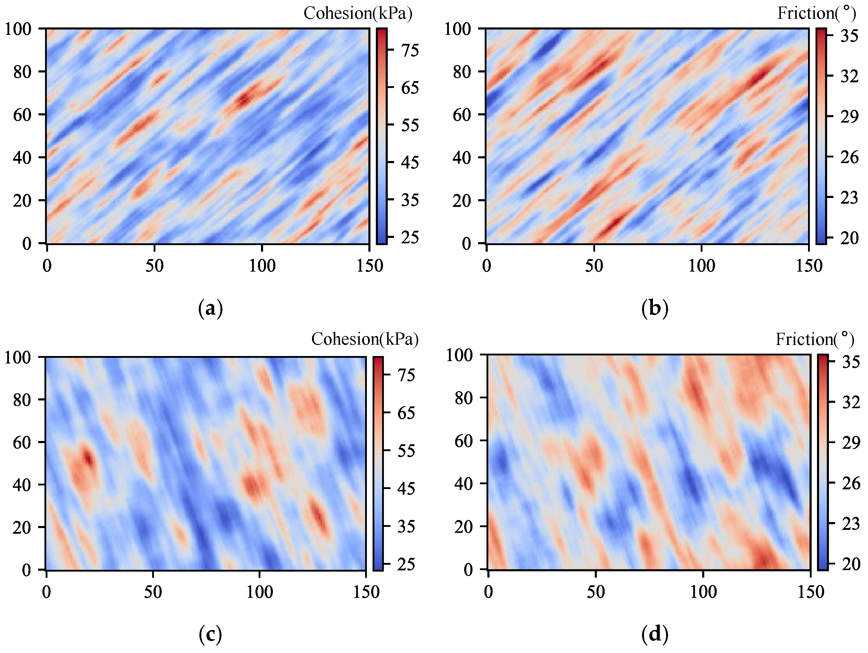
Figure 2.
Flowchart of the CRF construction method.
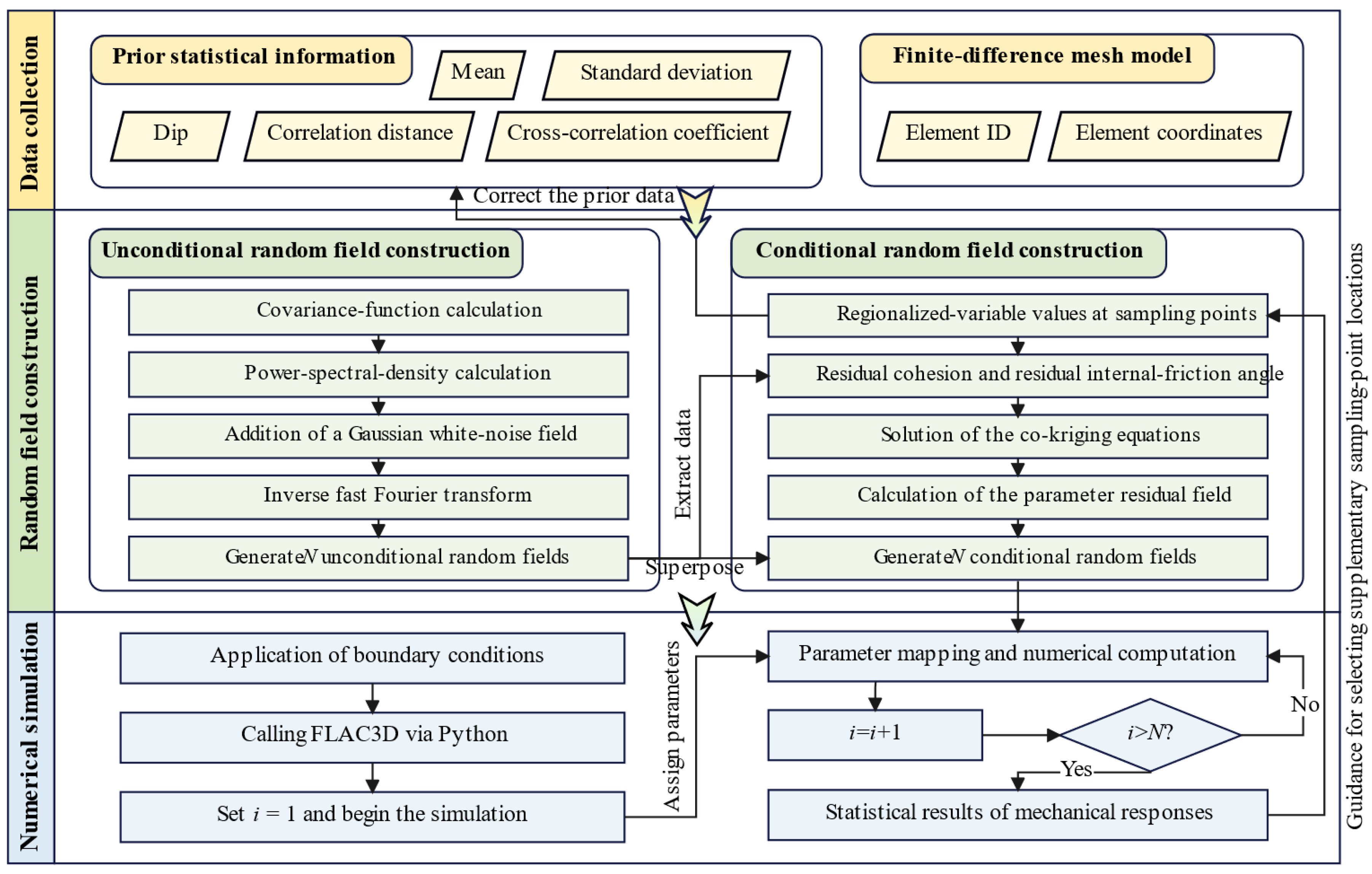
Figure 3.
Numerical slope model adopted in the case study.
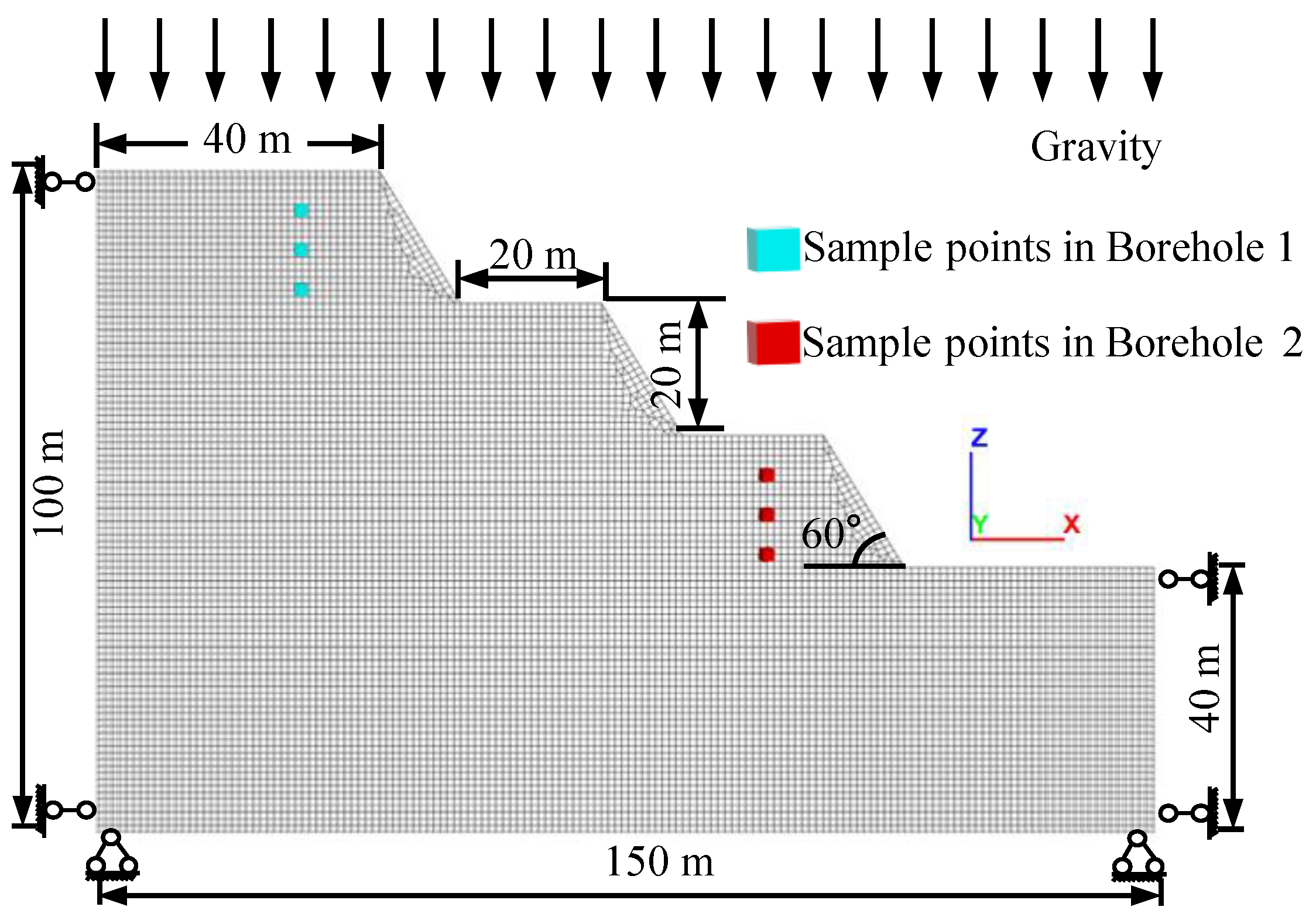
Figure 4.
The anisotropic URFs: (a) , dip 15°; (b) , dip 15°; (c) , dip 30°; (d) , dip 45°; (e) , dip 60°; (f) , dip 75°.
Figure 4.
The anisotropic URFs: (a) , dip 15°; (b) , dip 15°; (c) , dip 30°; (d) , dip 45°; (e) , dip 60°; (f) , dip 75°.
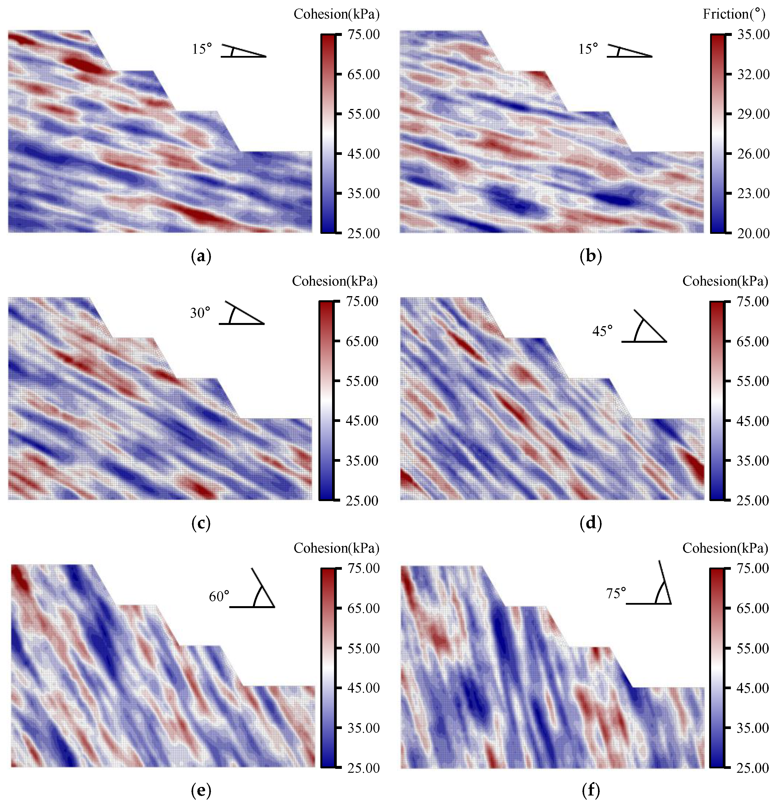
Figure 5.
Nine representative failure modes: (a) M1; (b) M2; (c) M3; (d) M4; (e) M5; (f) M6; (g) M7; (h) M8; (i) M9.
Figure 5.
Nine representative failure modes: (a) M1; (b) M2; (c) M3; (d) M4; (e) M5; (f) M6; (g) M7; (h) M8; (i) M9.
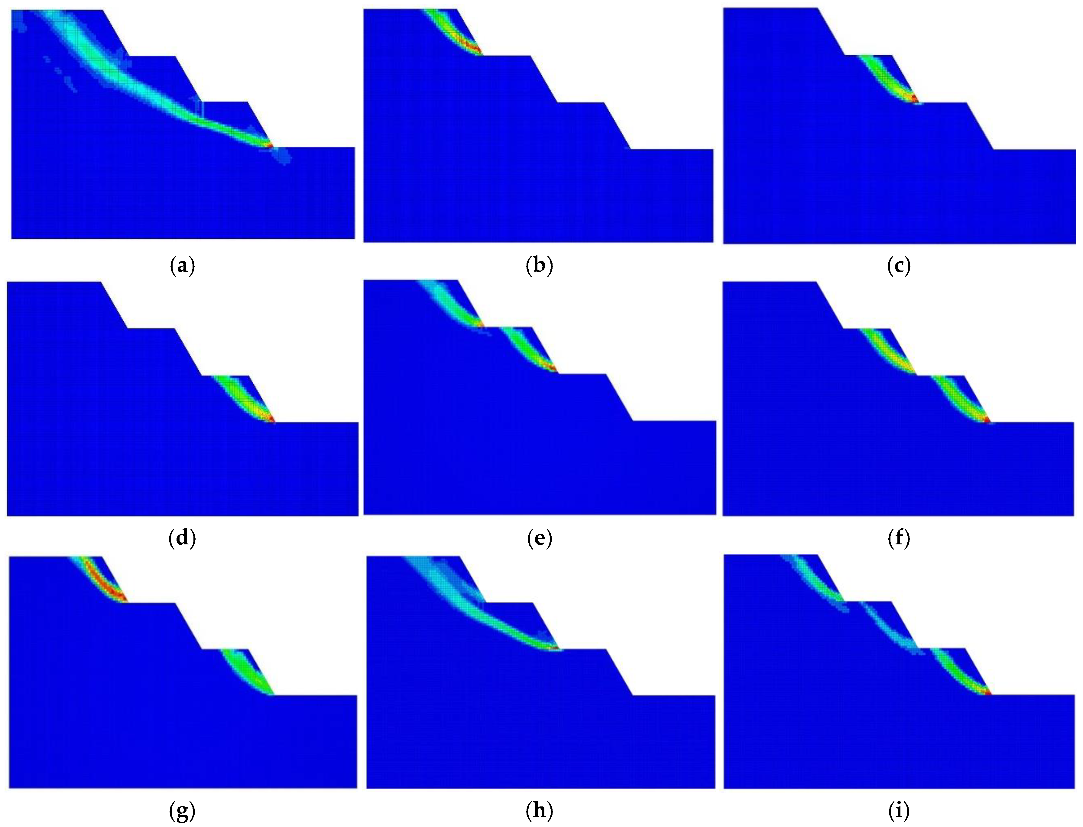
Figure 6.
Failure-mode proportions and mean safety factors of the slope under different bedding-dip angles for the URF: (a) percentage distribution of failure modes; (b) average safety factor.
Figure 6.
Failure-mode proportions and mean safety factors of the slope under different bedding-dip angles for the URF: (a) percentage distribution of failure modes; (b) average safety factor.
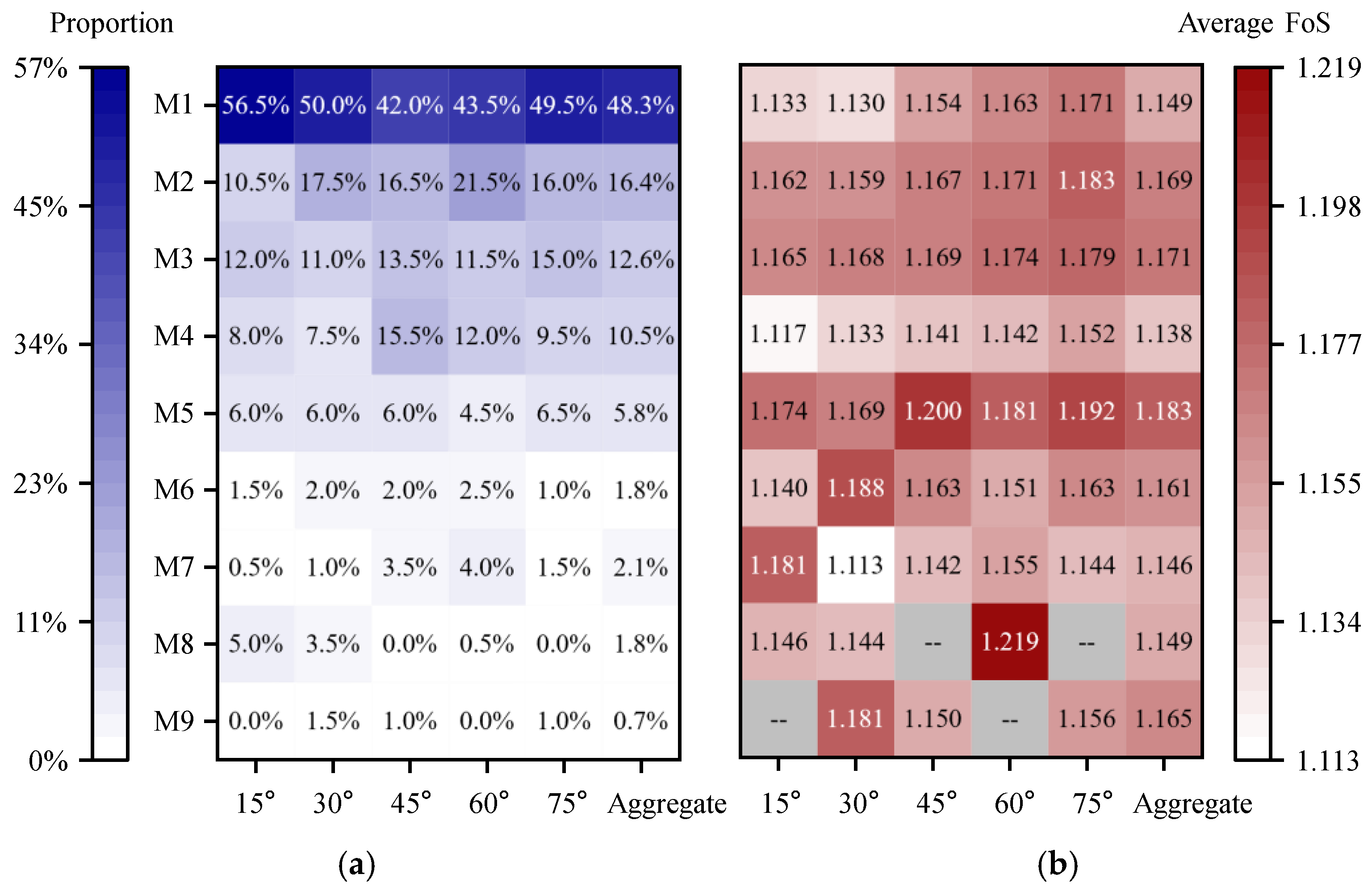
Figure 7.
Evolution from localized failure to global collapse: (a) bedding dip 15°; (b) bedding dip 75°.
Figure 7.
Evolution from localized failure to global collapse: (a) bedding dip 15°; (b) bedding dip 75°.
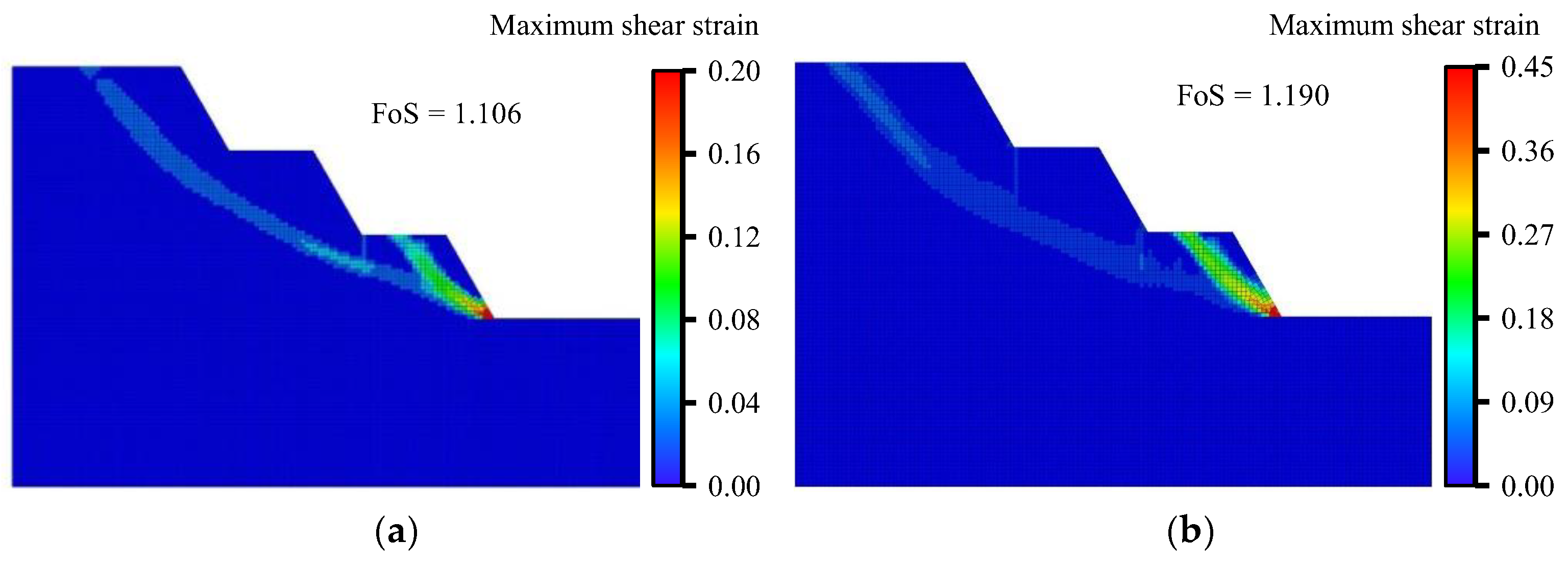
Figure 8.
Mechanical-parameter random fields at a bedding dip of 45° under different settings: (a), (b) URFs of and with = −0.2; (c), (d) IRFs of and with = 0.
Figure 8.
Mechanical-parameter random fields at a bedding dip of 45° under different settings: (a), (b) URFs of and with = −0.2; (c), (d) IRFs of and with = 0.
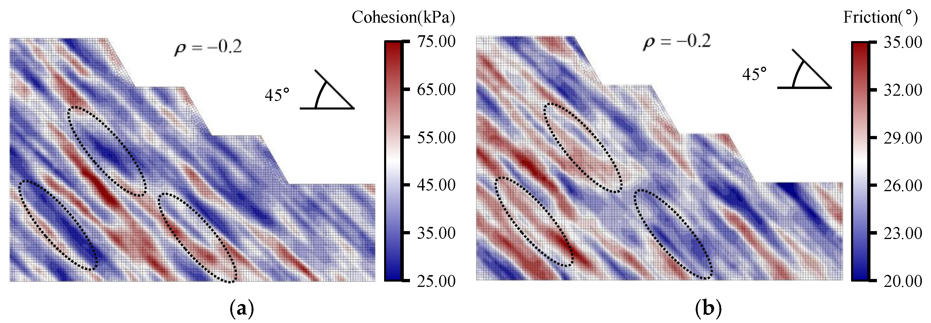
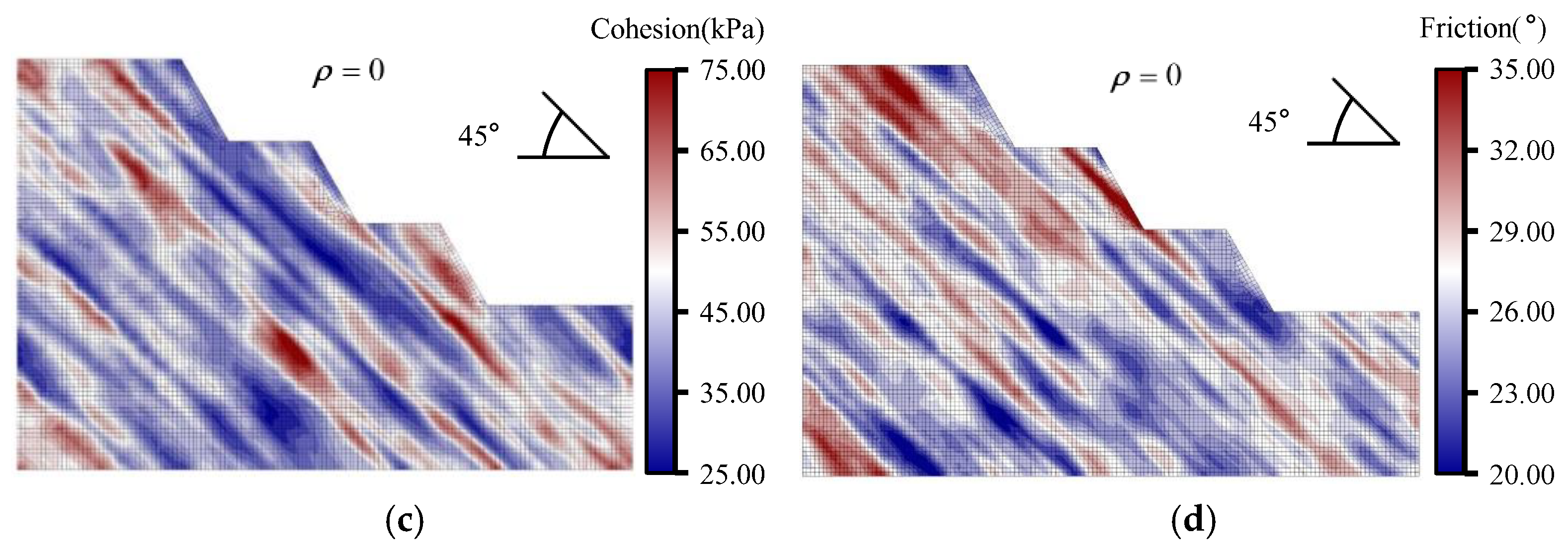
Figure 9.
Statistical results for the IRF at different bedding-dip angles: (a) matrix of failure-mode proportions; (b) matrix of mean safety factors; (c) ratio of failure-mode proportions for the IRF versus the URF; (d) ratio of mean safety factors for the IRF versus the URF.
Figure 9.
Statistical results for the IRF at different bedding-dip angles: (a) matrix of failure-mode proportions; (b) matrix of mean safety factors; (c) ratio of failure-mode proportions for the IRF versus the URF; (d) ratio of mean safety factors for the IRF versus the URF.
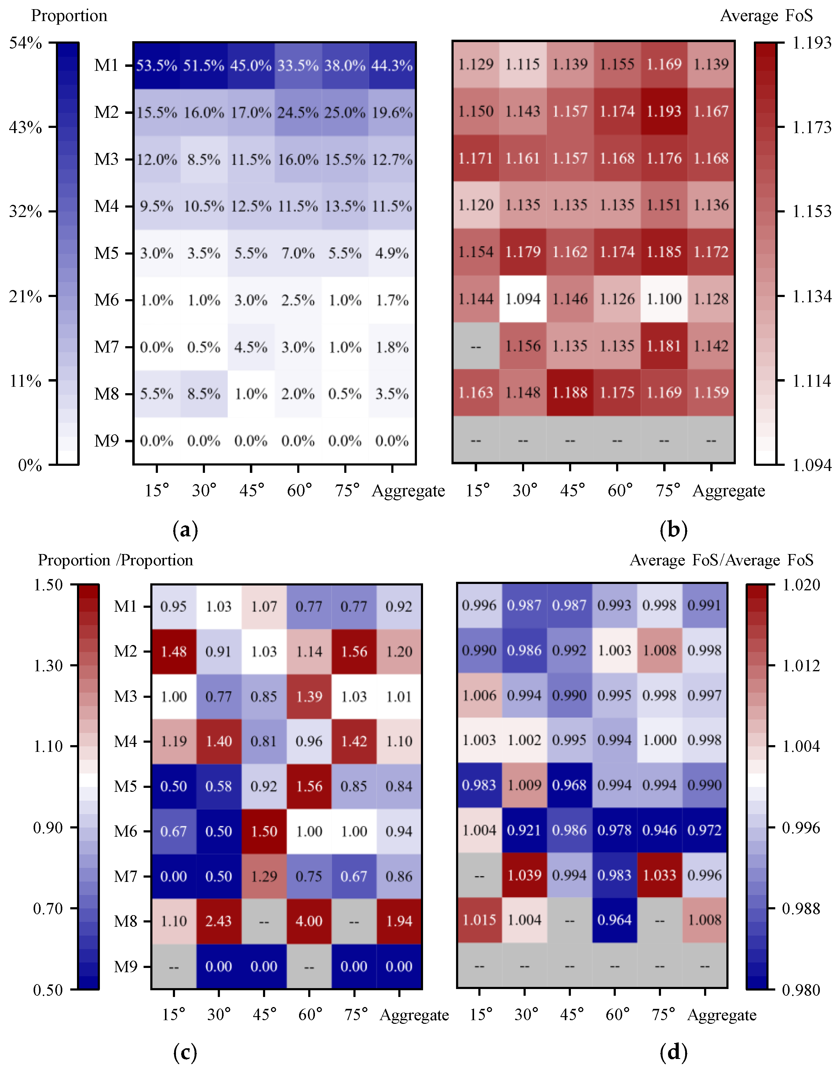
Figure 10.
CRFs of mechanical parameters with = −0.2: (a), (b) CRFs of and at a bedding dip of 30°; (c), (d) CRFs of and at a bedding dip of 60°.
Figure 10.
CRFs of mechanical parameters with = −0.2: (a), (b) CRFs of and at a bedding dip of 30°; (c), (d) CRFs of and at a bedding dip of 60°.
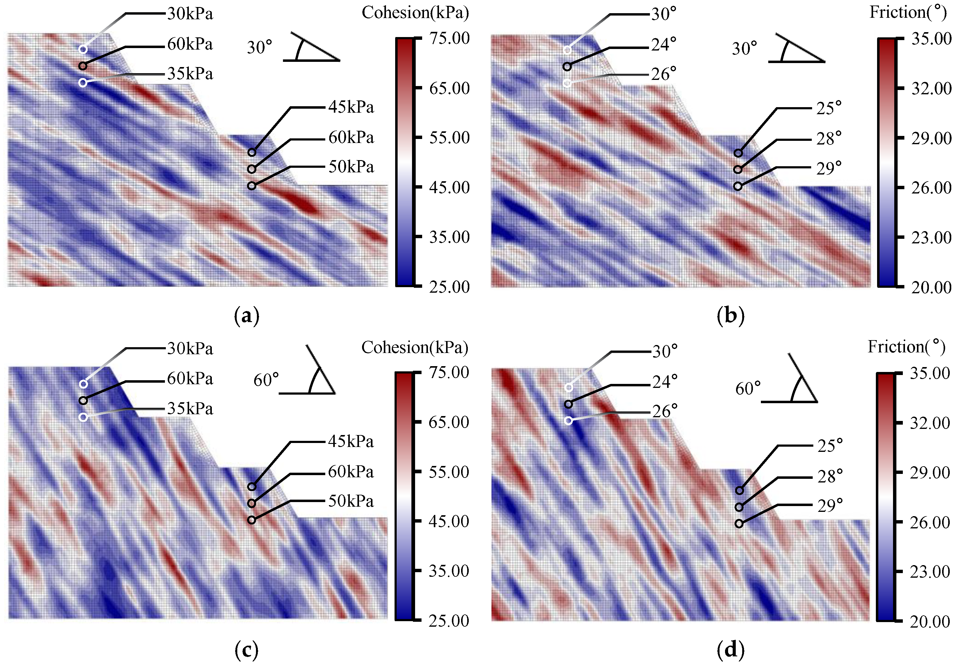
Figure 11.
Statistical results for the CRF at different bedding-dip angles: (a) matrix of failure-mode proportions; (b) matrix of mean safety factors; (c) ratio of failure-mode proportions for the CRF versus the URF; (d) ratio of mean safety factors for the CRF versus the URF.
Figure 11.
Statistical results for the CRF at different bedding-dip angles: (a) matrix of failure-mode proportions; (b) matrix of mean safety factors; (c) ratio of failure-mode proportions for the CRF versus the URF; (d) ratio of mean safety factors for the CRF versus the URF.
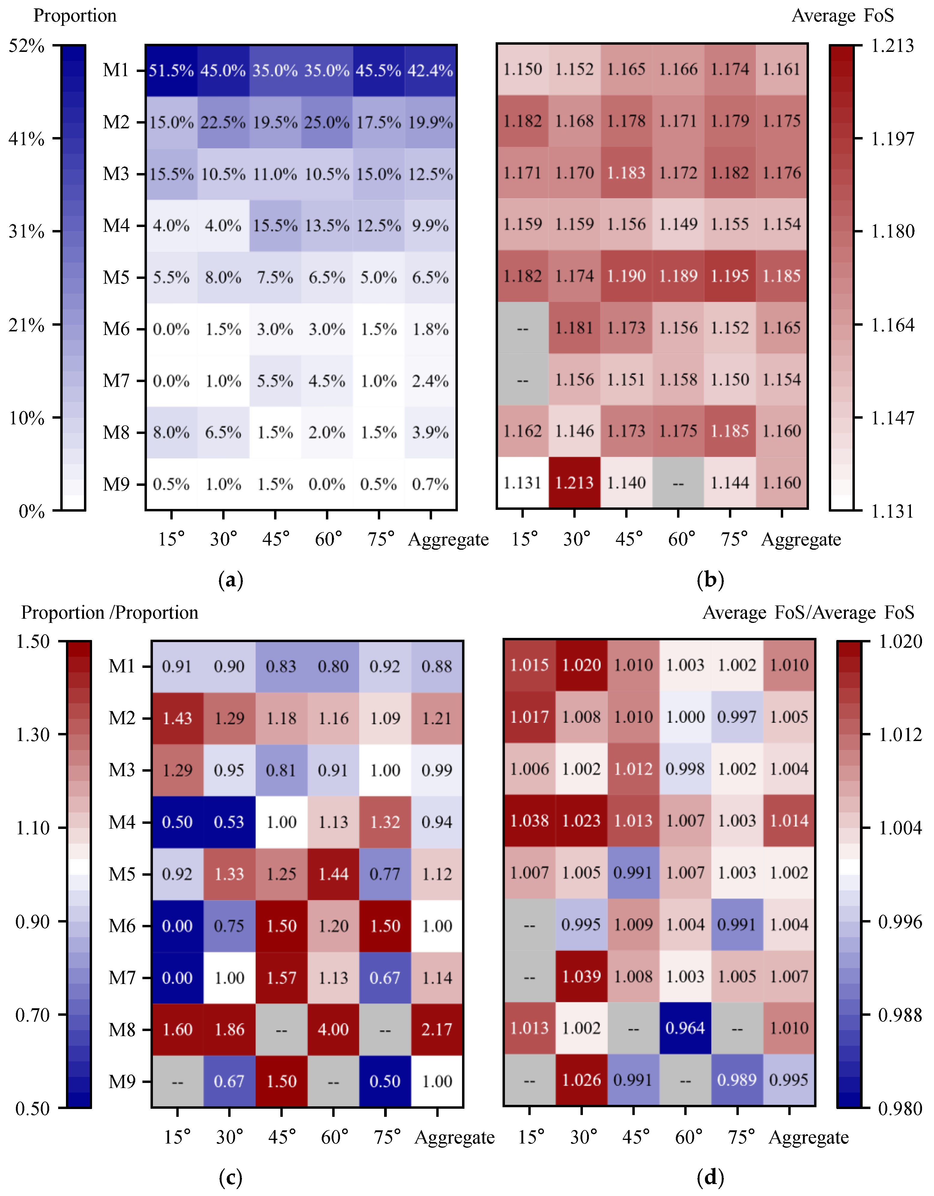
Figure 12.
Ridgeline plots of factor-of-safety distributions: (a) URF ( = −0.2); (b) IRF (= 0); (c) CRF (= −0.2); (d) comparison of the aggregate factor-of-safety distributions.
Figure 12.
Ridgeline plots of factor-of-safety distributions: (a) URF ( = −0.2); (b) IRF (= 0); (c) CRF (= −0.2); (d) comparison of the aggregate factor-of-safety distributions.
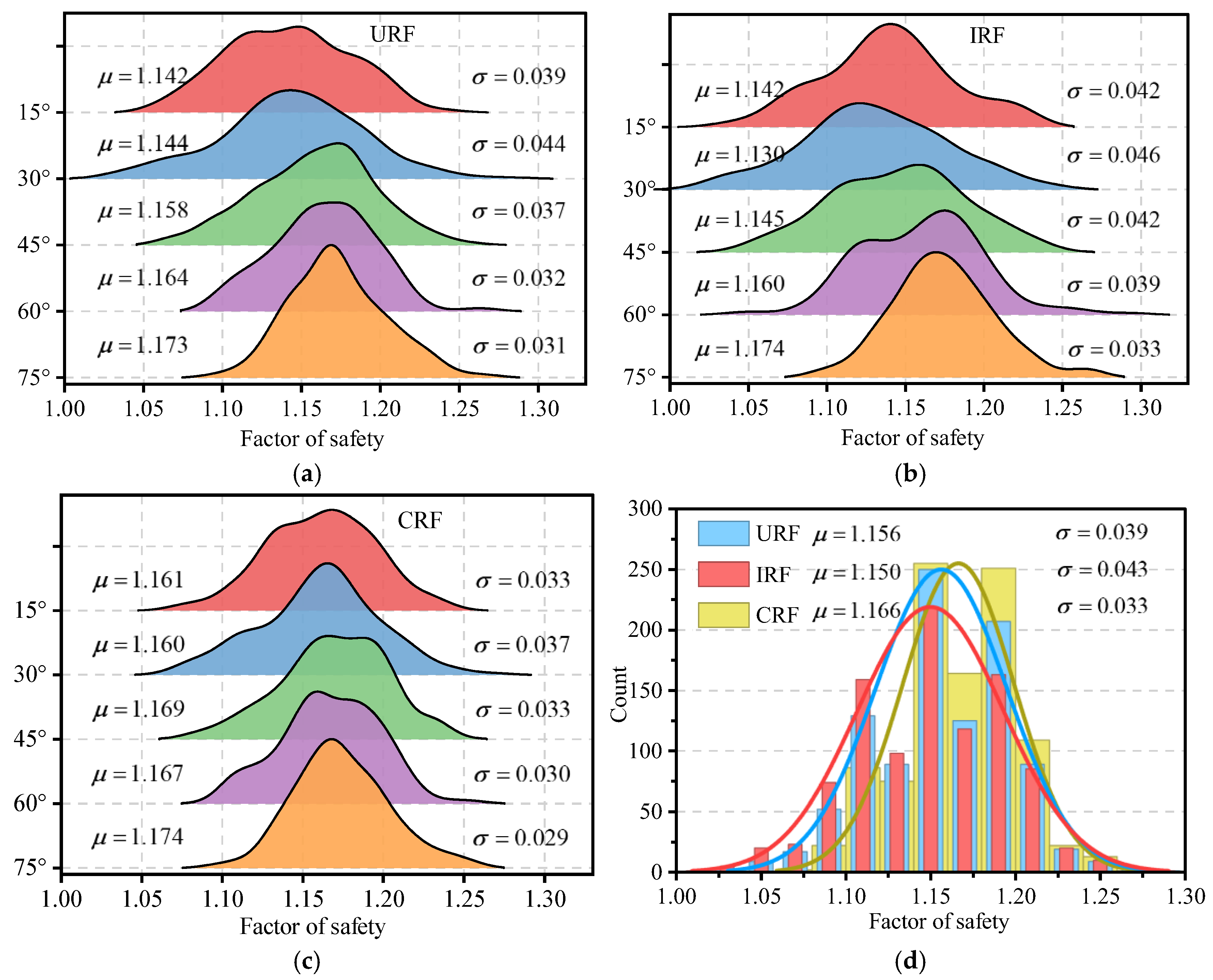
Figure 13.
Probability density function(PDF) plots: (a) cohesion, log-normal distribution (K–S test statistic D = 0.0273); (b) friction angle, normal distribution (K–S test statistic D = 0.0312); (c) summary of K–S test statistics; (d) cross-correlation statistics of mechanical parameters in URF versus CRF.
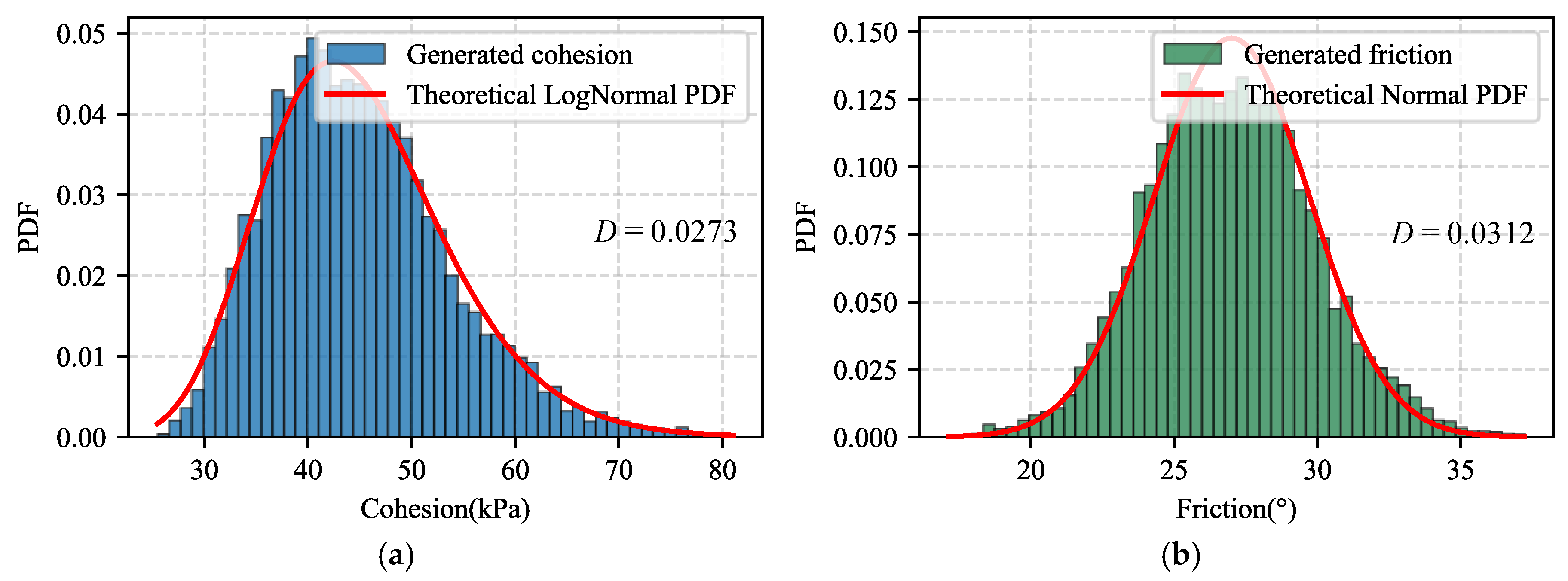
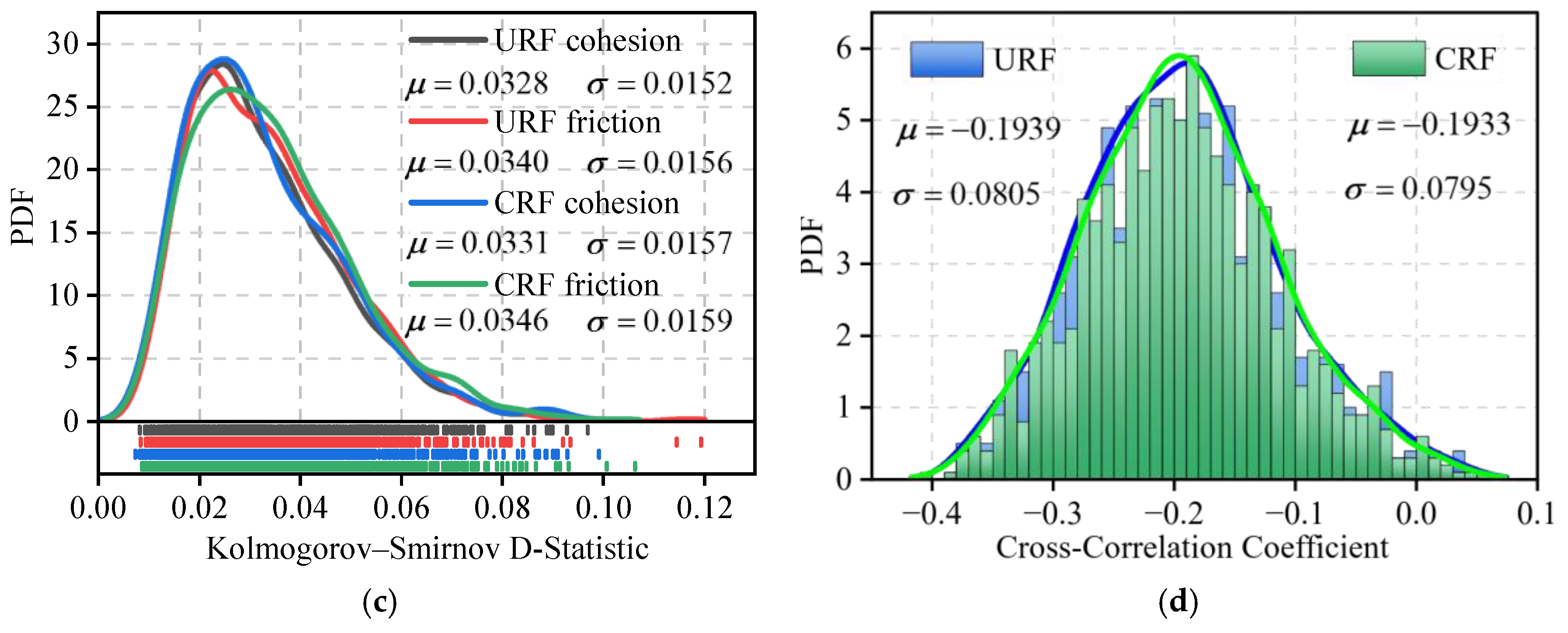

Table 1.
Prior statistical parameters of the rock–soil mass.
| Parameter | Unit Weigh (kN m⁻³) |
Elastic Modulus (GPa) |
Poisson’s Ratio | Cohesion (kPa) |
Friction Angle (°) |
|---|---|---|---|---|---|
| Mean | 23 | 1 | 0.25 | 45 | 27 |
| Coefficient of variation | — | — | — | 0.2 | 0.1 |
| Distribution type | Deterministic | Deterministic | Deterministic | Log-normal | Normal |
Disclaimer/Publisher’s Note: The statements, opinions and data contained in all publications are solely those of the individual author(s) and contributor(s) and not of MDPI and/or the editor(s). MDPI and/or the editor(s) disclaim responsibility for any injury to people or property resulting from any ideas, methods, instructions or products referred to in the content. |
© 2025 by the authors. Licensee MDPI, Basel, Switzerland. This article is an open access article distributed under the terms and conditions of the Creative Commons Attribution (CC BY) license (http://creativecommons.org/licenses/by/4.0/).
Copyright: This open access article is published under a Creative Commons CC BY 4.0 license, which permit the free download, distribution, and reuse, provided that the author and preprint are cited in any reuse.


