
Submitted:
23 July 2025
Posted:
24 July 2025
You are already at the latest version
Abstract
This study attempts to identify the most appropriate clustering algorithm for marketing and other fields that use them because identifying and classifying customers based on their needs and behaviors is essential, which is interpreted by big data science. However, before this, we must implement appropriate segmentation among customers. In this study, based on the opinions of famous faces such as Kotler, Porter, and Drucker about segmentation, information from 460 samples was collected in the form of seven variables by surveying consumers using standard scientific questionnaires. With the use of routine statistics, the validity and reliability of the data were examined and confirmed. Then, with two data mining platforms, Weka and RapidMiner, data clustering was implemented with thirty algorithms at different ranges. However, to compare with other studies, statistics were used more for analysis, and due to the non-normality of the data, non-parametric statistical methods such as Kruskal-Wallis, which is the non-parametric equivalent of the ANOVA test, and DSCF as a post-hoc test were used in addition to a Silhouette index. Finally, based on the statistical index of effect size, which is used in meta-analysis studies to compare results, the outputs were examined and proved that, except for the farthest-first algorithm, others do not show significant values in the seven mentioned variables. This means that for all data that have an abnormal shape on the Likert scale, the arrangement from the outside to the center of the cluster seems to be the most appropriate method for classifying customers.
Keywords:
machine learning
; comparison clustering
; Dwass-Steel-Critchlow-Fligner
; nonparametric data
1. Introduction
The clustering technique has been around for over half a century, but there is still capacity for improvement. A frequently asked question is: what type of clustering is appropriate to use? Studies have compared various clustering methods; however, when dealing with multiple heterogeneous variables and different types of data—such as binary, nominal, ordinal, and continuous variables—direct comparisons cannot be made across varying sample sizes without considering effect sizes and error values [1]. Therefore, we aim to identify the best type of clustering for Likert scale data by utilizing data mining and statistical methods, alongside real data collected from male massage consumers. One application of clustering is in marketing.
As noted by D’Urso (2015), effective segmentation through appropriate feature selection is crucial for market success. Accurate segmentation enables a company to gain strategic advantages, while irrelevant variables disrupt the process, wasting resources and leading to divergence from goals [2]. The application of clustering in marketing was first introduced by Saunders in 1980 [3]. His findings indicate that cluster analysis is valuable for segmenting consumer markets using variables such as needs, attitudes, and lifestyle. Other approaches, including benefit bundles and psychological variables, have also been employed. Recent advancements in clustering methodologies, such as flexible and componential segmentation, are under investigation. Cluster analysis has also proven useful in experimental settings and product positioning, with many researchers implementing clustering techniques in their publications.
Market segmentation, as defined by Kotler (2018), Pitts, and Stotlar (2013) [4,5], is “dividing a market into distinct groups of buyers who have different needs, characteristics, or behaviors and who might require separate marketing strategies or mixes.” It is a crucial component of market targeting, with companies advised to focus on segments where they can create and consistently maintain significant customer value. Segmentation may involve four latent variables: Geographic factors (nations, regions, states, cities, neighborhoods, population density, and climate), Demographic factors (age, life-cycle stage, gender, income, occupation, education, religion, ethnicity, and generation), Psychographic factors (lifestyle and personality), and Behavioral factors (occasions, benefits, user status, usage rate, and loyalty status).
Although multiple methods for classifying and clustering data have been developed [6], there are still ambiguities regarding their correct application for the diverse objectives and types of data in the fields of marketing and economics [7]. This study aims to resolve this issue by identifying the most appropriate method based on empirical evidence, specifically through feedback from male massage consumers and the application of clustering techniques.
What distinguishes this research is the use of multiple algorithms for comparative analysis, providing a comprehensive perspective, and results derived from scientifically validated methods based on accepted metrics, enhancing reliability. Unlike other investigations, this research incorporates innovative methodologies and emphasizes valid data grounded in standard statistical indicators, a facet often underrepresented in other studies.
The credibility of the data facilitates a more robust generalization of findings to the broader population. This research focuses on comparing clustering methods to identify the most suitable approaches for Likert scale scientific data, combining data mining techniques from computer science with quantitative research methods in the humanities and sciences to address these ambiguities.
2. Related Works
The First Comparison of Clustering Methods with the Title of “Comparison of Some Cluster Analysis Methods” Made by Gower in 1967[8], over the Time, with spread of of Algorithms Growth, Some Scattered Comparisons Were Made, the Most Remarkable of Which Will be Introduced in the Following. Rodriguez et al (2019) Believe That the Spectral Approach Outperforms Other Techniques with Exceptional Performance. However, the Hierarchical Method is Highly Sensitive to the Number of Features, Which Affects Its Effectiveness. Algorithms Show Different Levels of Performance Depending on the Number of Features Used [9]. Hennig (2021) Researches Outcomes Concerning the Portrayal of the Data Through Centroids Reveal That K-Means Surpasses Clara When Examining Squared Euclidean Distances Relative to the Centroid. Conversely, in Terms of Unsquared Distances, Clara Demonstrates Superiority [10].Kaya and Schoop (2022) in Their Study found out that the Combination of Internal and External Evaluation Measures Can Lead to Different Cluster Results. The K-Means (OS; K = 5) Performs Well with External Evaluation Measures, while K-Means (PCA; K = 7) is Rated Third Best by Cohen’s Kappa and F-Score, But Lacks Internal validation. Some Methods, Like X-means and DBSCAN (OS), Show Mediocre Results. It’s Important To consider Both Internal and External Evaluations to Ensure Accurate Cluster Results [11].
Costa et al (2023) in Comparing Clustering Methods, examine the Performance of Distance-Based Partitioning Methods on Various Simulated Data Sets. Eight Methods Were Evaluated, Including Approaches for Constructing Dissimilarity Matrices, Adapting K-Means to Mixed Data, and Reducing Variables. The Benchmark highlighted similarities and differences in algorithm performance, with KAMILA, FAMD/K-Means, and K-Prototypes Standing Out as Top Performers and [12]. In Sepin et al (2024) study, K-means clustering, OPTICS, and Gaussian mixture model (GMM) clustering were compared on vibration datasets, examining the effect of feature combinations, PCA feature selection, and the number of clusters. The results showed that averaging and variance-based features were more effective than shape-based features, and clustering with K-means was slightly better than GMM [13].MoreTechnical Details of These Papers are Presented in the Table 1
3. Methodology
The paradigm of this study is post-positivism, and its approach is quantitative. The target population consists of male massage service consumers in Iran. The Steps of Data Mining Include Collecting Data, selecting a Suitable Attribute for the Algorithm, running it and receiving output, finding the best Cluster and finally mining additional Data from the Output. Comparing Methods Add to the Chart According to the Figure 1
A cluster sampling method was employed to obtain a representative sample. To compare cluster variances, a maximum of 20 clusters was anticipated, and the sample size was determined using formula-based methods with G*power software Figure 2 [14,15]. with a maximum of Twenty number of clusters and a minimum of two clusters, along with seven variables having an effect size of 0.1, a confidence level of 95%, and a power of 0.95, the required sample size was calculated to be 460 members.
3.1. Instruments:
For Measuring the Current Variables, Data Collection Instruments Developed in Recent Years Were Selected, Such as the Developed Scales [16,17,18]. These Instruments Underwent Face Validity and Content Validity tests. Subsequently, the Final Questionnaire Was Developed Based on the Reflective Nature of the Items [19], Which Included Demographic Questions and Items With a 5-Point Likert Scale. in Pre-Processing and Primary Reliability Measurement and For Post-Hoc Tests Were Used to Calculate and Compare Clustering Methods, JAMOVI 2.5 Used to Calculate and Compare Clustering Methods and Weka 3.9.6 With Its Plugins and RapidMiner 9.1.0 With its Plugins as Data Mining Platform’s. The Reason of Using These Software’s, Primarily Their Free Availability, Which Makes Them Accessible to Everyone Additionally, both are User-Friendly Thirdly the Open-Source Library of All Methods (Table 2) and Forth in the Clustering Section are Different and Has Overlap With Each Other، and Use Them Helps to Spread Research in More Fields.
3.2. Performance
3.2.1. First Step
After collecting and preparing Data, Clustering Operations Were Performed for Each Algorithm with Varying Quantity until the Initial Clustering Threshold Without Any Specific Membership Was Determined.
3.2.2. Second Step
The Quality of the Generated Clusters Was Evaluated in Terms of the Number of Members and Recommend That Clusters With 2% Or Less Compared to the Total Sample Population, be Considered Poor Clustering, and Clusters With 5% Until 2% member initial be Considered Near to Poor. After Identifying This Range, it Should be Further Examined Using the ANOVA Test to Determine Which Clusters are Similar, This Test is Most Known for Data Miners as F Test.
This test could be run if data known normal by one of D’Agostino, Anderson-Darling, Shapiro-Wilk, or Kolmogorov-Smirnov tests so the results of ANOVA Test Determine Which Clusters are Similar, Indicating Poor Clustering Quality. If Data Known as Un-normal and There is More Than Two Groups to Compare and Many Variables; the Non-Parametric Equivalent Test Means Kruskal–Wallis Test That Must be Implemented.
N;is the total number of observations across all groups
g; is the number of groups, n_i is the number of observations in group i, ; is the rank (among all observations) of observation j from group i,
is the average rank of all observations in group i, is the average of all the [20].
3.2.3. Third Step
After Narrowing Down the Remaining Choices, the Post-Hoc DSCF[1] Test Precisely Identifies Which Clusters Have the Least Similarity Between Them, as it Compares Each Cluster Pair. it Necessitates the Recalculation of Ranks for Every Treatment Combination. the Statistic is Computed for Each of These Combinations. This Test All-Treatment Multiple Comparison Procedure is Based on the Maximum of the Studentized Two-Sample Wilcoxon Statistics, Computed Over All Pairs of Samples. for Each Pair let
where ψ(t)=1 if t>0 and 0 otherwise, be the rank sum associated with the Sample When Ranked with Sample j. in Addition, let
denote the studentized Wilcoxon statistic (multiplied by √2). for Each Pair i, j with 1 ≤ i < j ≤k, the Steel-Dwass procedure declares that whenever Where Is Chosen so That
and the Probability (-) is Computed Under the Null Hypothesis Assumption an Expression Analogous to (8) is Given for the Case When Not All the are Equal, That Utilizes the Same value of . it is Used to Derive the Simultaneous Confidence Intervals for the Differences 1 ≤ i < j ≤ k, and to show that the procedure satisfies property (Control of the maximum type I error rate). Also, for a large Sample Approximation for is Provided Below, Which Ensures That the Probability in (8) Has Limit for Equal n_i, and limit ≤ when the sample sizes are unequal.
Let
where
And . note that under the null hypothesis, the component vectors
both have limiting multivariate normal distributions with mean vector 0 and the same covariance matrix, when
and for the covariance structure). Thus, for large sample sizes, we may take
thereby ensuring that the probability in (8) has limit a for equal sample sizes, and limit < a for unequal sample sizes. This gives the standard approximation for large and equal sample sizes. the conservative nature of this result for unequal is new. as with Tukey-Kramer, the probability will generally be quite close to [21].
3.2.4. Forth Step
the Optimal Clustering is Determined Among the Remaining Options Using the Silhouette Test who offered by Rousseeuw(1987) [22].
3.2.5. Fifth Step
And for Scientific Result’s Comparison, The Effect-Size Index Used at the End. it is Expressed to Highlight the Practical Significance and Implications for Information Systems Research, it is Essential for Statistical Studies to Consistently Report Effect Sizes.
sum of squares for the effect ;sum of squared errors
; mean square of the effect, ;mean square error, ;the total sum of squares, ;degrees of freedom for the effect by Detailing Effect Sizes, Researchers Not Only Demonstrate the Applicability of Their Findings But Also Facilitate Evidence-Based Practitioners in Comparing the Effects of Various Interventions Across Different Studies [12,23]. Fritz et al (2012) about Importance of Effect Sizes express that Effect sizes serve several critical functions: They help determine the practical or theoretical importance of an effect. They allow for the comparison of effects across different studies. They assist in power analysis, which is crucial for determining appropriate sample sizes in future research [24].
4. Results
After performing clustering for each algorithm and identifying the optimal cluster, the final results for the best cluster in each algorithm are presented in Table 3 (Appendix).
Six normality tests concluded that for large sample sizes, the Shapiro-Wilk and D’Agostino-Pearson tests are the most powerful [25] ,Also Shapiro-Wilk Test Is The Most Powerful Test Followed By The Anderson-Darling Test [26]. According to these tests, Data does not follow a normal distribution; however, all indexes Table 4(Appendix) yielded valuable results. After conducting the KMO and Bartlett’s test to assess sample adequacy and sphericity, a KMO value of 0.784 was obtained, exceeding the threshold of 0.6. Researchers have confirmed that the number of observations is sufficient for factor analysis [27]. The sphericity of relationships among indicators has been validated as crucial for factor analysis due to the significance of the Bartlett test (Sig = 0.001 < 0.05).
The Shapiro-Wilk results indicated abnormality in the data, as shown by high skewness and kurtosis. Consequently, nonparametric methods were employed. The equivalent nonparametric test for normal analysis of variance is the Kruskal-Wallis test, which assesses the null hypothesis that the clusters (groups) are similar. However, it only indicates whether there is a difference among at least one of the clusters, necessitating a post-hoc test to compare the clusters individually. The DSCF post-hoc test can determine which clusters are similar or different by compairing each pair of clusters. This test is available in NCSS, SAS, Jamovi, JASP, R packages, and Excel macros, and it is noted to be more robust and effective for large datasets compared to the Conover-Iman or Wilcoxon rank tests [28,29,30,31]. Once the optimal cluster is identified, the next step is to calculate the effect size of the variables in clustering, as shown in Table 5 (Appendix).
5. Discussion
As mentioned in Section 1 of the literature review, clustering based on central tendencies (such as the mean) is inappropriate for binary data (such as gender or employment status) and ordinal data (such as education levels) due to the meaningless nature of calculating averages for this type of data. Therefore, these were excluded from the evaluation. We only considered the 5-point Likert scale questionnaire responses for standardization purposes, which some studies in the literature have overlooked. In the initial clustering phase, G-Means, BANG-File, and OPTICS were not executed; instead, numeric attributes were first adopted. The resulting clustering outputs for agglomerative (919 clusters), hierarchical (459 in the first step and 1 in the second), and top-down algorithms (34 clusters, with 23 lacking members) were imbalanced and unacceptable. The similarity in clustering results between the X-means and Fast K-Means algorithms in RapidMiner indicated that they differed only in name while having the same structure. Consequently, X-Means was disregarded in RapidMiner, and its output was recorded and utilized in Weka.
This method requires testing all indices, meaning that each time, one variable is considered as an index to calculate the distance to other variables. For K-Means, a mixed measure was chosen. The clustering process began with two clusters, one of which was poorly formed, ultimately resulting in 16 clusters. The poorly performing cluster began at 12 clusters, with 38 clusters showing no membership. Except for the 2 and 3 clusters, all remaining clusters were similar, sharing common members. The final step revealed that a higher silhouette index was associated with 2 clusters, with observed similarities in courtesy, aesthetics, and perceived value indices. In the K-Means H2O clustering process, a decline in clustering quality was noted starting at 11 clusters, with poor clustering observed at 17 clusters. A cluster without membership appeared at 30 clusters. Again, aside from the 2 and 3 clusters, all other clusters were similar, with a higher silhouette index associated with 2 clusters, showing similarities in access, aesthetics, perceived value, courtesy, and loyalty indices. For K-Means Kernel, clustering quality began to deteriorate at 11 clusters, and poor clustering was observed at 13 clusters, with a cluster lacking membership appearing at 60 clusters. This evidence suggests that this method behaves similarly to its counterparts, except it fails to reveal clusters without membership. Except for the 2 and 3 clusters, all clusters were similar, and a higher silhouette index was linked to 2 clusters, with dissimilarities observed only for the access index.
For K-Means Fast, clustering quality decreased starting at 11 clusters, with poor clustering observed at 13 clusters and clusters without membership noted at 38. This evidence suggests that this method behaves like K-Means. Except for the 2 and 3 clusters, all others were similar, with a higher silhouette index belonging to 2 clusters. Unsimilarity between clusters was observed only for courtesy, aesthetics, and perceived value indices. For the execution of the K-medoids algorithm, instead of using the average of the data, the mode was calculated and utilized for clustering. This algorithm operates based on the median index.
Additionally, we observed that the arrangement or order of variables does not significantly impact the clustering result, as this model performs clustering based on the dataset itself. Poor clustering began at 9 clusters and continued until 16 clusters, with no membership observed at 17. Except for the 2, 3, and 4 clusters, all other clusters were similar, and the higher silhouette index belonged to the 4 clusters, with dissimilarity between clusters observed only for attitude.
There are two adjustable variables in the DBSCAN model: epsilon and the minimum points. Different values for these variables were tested; however, no improvement in clustering quality was observed. This means that some members did not belong to any cluster and were referred to as noise. For the random algorithm, clustering quality decreased starting at 11 clusters, with poor clustering observed at 26 clusters and clusters without membership noted at 46. This method behaves similarly to K-Means and K-Means Kernel, with all clusters being similar, resulting in the silhouette test not being conducted. For Fuzzy C-Means, clustering quality decreased starting at 8 clusters, with poor clustering noted at 12 clusters and a cluster without membership observed at 13. This suggests that this method is sensitive; except for 2 and 3 clusters, all others were similar, with a higher silhouette index belonging to 2 clusters. Unsimilarity between clusters was observed only for aesthetics, courtesy, access, attitude, and perceived value. In the Flatten method, poor clustering appeared at 2 clusters, with a cluster without membership observed at 8, indicating that this method is unfriendly to Likert scale data. For the Canopy method, there are three adjustable variables: T1, T2, and seeding quantity. Different values for these variables were tested. The default values are seeding = 1, T1 = -1.25, and T2 = -1.0. T1 represents the distance to use; values less than 0 are taken as a positive multiplier for the T2 distance, which also represents distance. Values less than 0 should be set using a heuristic based on the attribute’s standard deviation, making it effective only during batch training. Since these numbers result from scientific work by the producers, we did not alter their relationships; instead, we adjusted them by adding or subtracting from this ratio. These changes did not affect the output results, but modifying the seeding made the results distinguishable. Clusters in field 10 are weak, while in field 1, they are better.
Consequently, field 10 is gradually being abandoned as the number of clusters increases. Poor clustering started at 4 clusters, except for 2 and 3 clusters. All others were similar, with a higher silhouette index belonging to 2 clusters, with 5 seeds, and unsimilarity between clusters was observed for access, courtesy, perceived value, and Quality. For Cascade K-Mean, there is only one adjustable variable for seeding quantity, with a default of 1. Different values for seeding were tested, but there was no difference between them, even in the silhouette output. Thus, the higher silhouette index belonged to 2 clusters. For CLOPE, one condition for implementing this method is that the data must be nominal, and there is only one adjustable variable, repulsion. Different values were tested for it. All outputs had clusters without membership, indicating that this method is not appropriate for Likert data.
For Cobweb, there are two adjustable variables: Acuity and Seeding. Different values were tested for them. The default value for Acuity is 1, and for Seeding, it is 42. It was observed that clusters 1, 2, 3, 32, and 33 were similar, indicating that this method is not appropriate for Likert data. For EM, although it is automated, the number of clusters is regulative, similar to K-Means. A decrease in clustering quality started at 11 clusters, with poor clustering at 13 clusters. Clusters without membership were observed at 49. Except for clusters 2, 3, and 5, all clusters were similar, with a higher silhouette index belonging to cluster 2, and unsimilarity between clusters was observed for Access, Courtesy, and Perceived Value indexes. For the farthest first, the only regulative index is Seeding. The best seeding is considered a rise in that seeding. Clustering started at 4 clusters, with poor clustering at 2 clusters, and clusters without membership were observed at 17. Except for 2 clusters, all clusters were similar, with a higher silhouette index belonging to it, and similarity between clusters was observed for all indices.
For Gen Clust Plus Plus, there are three adjustable variables: Initial Population size, Generations, and Seeding. Different values were tested for them. The default value for Initial Population size is 30, Generations quantity is set to 60, and Seeding is 10. There are only three options that yield similar clusters and a higher silhouette index. They belong to 2 clusters with an Initial Population size of 20, a Generations quantity of 60, and a Seeding of 10. Unsimilarity between clusters was observed only for Courtesy and Attitude indexes. Additionally, there was no significant difference observed when changing Generations quantity values. For LVQ, there are two adjustable variables: Learning Rate and Cluster Quantity. Different values were tested for them. The default value for the Learning Rate is 1.0. The best output was observed at a 0.5 Learning Rate for two clusters. This rate was tested on other cluster quantities. Except for clusters 2, 3, and 4, all others were similar, with a higher silhouette index belonging to cluster 2 with a 0.5 Learning Rate, and unsimilarity between clusters was observed, except for Loyalty.
For Density-Based Clustering, poor clustering was observed at 13 clusters, with clusters without membership observed at 51 clusters. Except for 2 clusters, all clusters were similar, with a higher silhouette index belonging to 2 clusters, and unsimilarity between clusters was observed for Aesthetics, Perceived Value, and Courtesy indexes. For the SOM algorithm, known for automation decisions, the only regulative index is the Learning Rate. Different values were tested for it. Overall, there are only 4 cluster outputs, and all of them were similar, leading to disappointing results.
For sIB, clustering quality decreased starting at 15 clusters, with poor clustering observed at 20 clusters. Clusters without membership were noted at 27 clusters, except for the 2 and 3 clusters tested; others were similar and had higher silhouette outputs, with the index belonging to 2 clusters. Unsimilar clusters were disappointing, except for loyalty. The only regulative index is seeding, with different values tested, showing the best results belong to 1 seeding. For X-Mean, the only regulative index is also seeding; different values were tested, and there were no differences between them, so the default was used. Clustering quality decreased starting at 12 clusters, with poor clustering at 17 clusters. Clusters without membership were observed at 31 clusters, and except for the 2, 3, and 5 clusters, all others were similar. The higher silhouette index belonged to 2 clusters, and unsimilarity between clusters was observed only for courtesy, aesthetics, and perceived value.
6. Conclusions
Based on this study and previous research, the Kruskal-Wallis test, when confronted with more than two independent groups across seven variables, cannot alone reveal the differences between the groups [32]. If the Kruskal-Wallis test indicates a significant difference among the groups, pairwise comparisons may be employed to identify specific differences, similar to the methodology utilized in a single-factor ANOVA. It is crucial to mitigate the risk of Type I error in this context. Given the settings configured in the G*power software, the sample size was determined to be 460 individuals, with the power obtained being 0.96. A power of 0.96 means there is a 96% chance that the test will correctly detect an effect in differences between clusters that exist. This high power indicates that the test is sensitive and has a low risk of missing true differences.
Based on this preface and referring to Table 5(Appendix), the group with the highest effect size (>0.9) is followed by K-Mean, K-Mean Fast, X-Mean, K-Mean H2O, Cascade K-Mean, Making Density, and Fuzzy C-Mean. Following them, sIB, EM, Canopy, LVQ, and Gen clust Plus Plus are known as good methods, while Farthest First, K-Mean-Kernel, and K-Medoid fall into the moderate group. Costa et al. (2023) express that “the worst performing methods were HL/PAM, Mixed K-Means, and Gower/PAM,” and PAM functions as k-medoids, so the results include Gen clust Plus Plus [12]. From the perspective of the variance index, which measures the similarity between members within clusters and the differences between members of different clusters, even sharing a single member between clusters is taken into account. Otherwise, the p-value, which indicates the measurement error, will not be significant. Therefore, although they all have high effect sizes, if the measurement error for all indicators is significant and less than 5 percent, the indicators can be considered desirable. The non-significance of the measurement error of a variable indicates that there are members common between clusters in the clusters created for that variable, suggesting that the clusters have not performed their function effectively.
The results are new and have not been previously observed in this comparison. Despite the abnormal data and the average inclination towards the center for normal data, two perspectives can be considered based on the obtained results. The performance of the algorithms in producing better clusters can be examined through the cumulative effect size and power index of each variable. The K-means clustering algorithms, except for the K-means kernel, demonstrate the best performance on some variables, as shown in Table 5(Appendix). These results align with the findings of Kaya and Schoop (2022) and Sepin et al. (2024) [11,13]. Although data types and comparison methods differ from those of Costa (2023) [12], the improved K-means algorithms still show the best performance and effect size. However, a significant limitation is that these algorithms cannot cluster all variables effectively, leading to overlapping members and suboptimal clustering shapes.
Additionally, the Fuzzy C-Mean algorithm ranks lowest among the evaluated methods. The results indicate that at the lowest levels, the Farthest First, K-Medoid, and K-Mean Kernel methods are also present. According to Table 5(Appendix), these methods fail to achieve significant accuracy in clustering, except for Farthest First, which effectively separates the data, although the effect size remains low. This suggests that the success of this algorithm may be due to its handling of abnormal data. This method sorts data from the farthest point, and abnormal data typically shows high kurtosis and skewness due to dispersion, giving it an advantage over methods based on central tendencies. Therefore, it is recommended to use the Farthest first algorithm for clustering non-normal data, as it produces more distinct and cohesive clusters. It is also advisable to select varying grain sizes to achieve optimal clustering. In study, the range was between 2 and 5, with a grain size of 2 resulting in the most dissimilar clusters. This advantage is appealing to data miners, though it may diverge from the preferences of statisticians, who prioritize the best resolution. Nevertheless, this does not diminish their value, and their effectiveness remains intact; changing the data type may necessitate an alternative approach from a data mining perspective, but it will not undermine the efficacy of the clustering methods.
Acknowledgments
The Author would like to express his gratitude to Professor Dr. Eibe Frank, Dr. Mark A. Hall, and Dr. Ian H. Witten for providing open access to the Weka and thanks very much Ingo Mierswa & Ralf Klinkenberg for providing open access to the RapidMiner Platform. Furthermore, He also would like to express his gratitude to the owners of Jamovi, G*Power and Zotero software’s for free access.
Appendix A

Table 3.
Optimum Clustering for Each Method.
| Cluster Metod | Quantity Of Cluster | Seeding | With Out Membership | Poor Cluster | Kruskal Wallis | DSCF | |
| K-Mean | 2 | - | no | no | Significant For Courtesy, Perceived Value, Aesthetics | Significant Courtesy-Perceived Value- Aesthetics | |
| K-Mean Fast | 2 | - | no | no | Significant For Courtesy, Aesthetics, Perceived value |
Significant For Courtesy, Aesthetics, Perceived value |
|
| K-Mean H2O | 2 | - | no | no | Unsignificant For at attitude | Significant For Access Aesthetics, Perceived Value, Courtesy, Loyalty |
|
| K-Mean Kernel | 2 | - | no | no | Unsignificant For Access, | Unsignificant For Access, | |
| K-Medoid | 4 | - | no | no | Significant All Except Loyalty | Significant For at attitude | |
| Fuzzy C-Mean | 2 | - | no | no | Significant For Aesthetics, Courtesy, Access, at attitude, Perceived value | Significant For Aesthetics, Courtesy, Access, at attitude, Perceived value - | |
| Canopy | 2 | 5 | no | no | Significant For Access, Courtesy, Perceived value, Quality | Significant For Access, Courtesy, Perceived value, Quality | |
| Cascade k-Mean | 2 | - | no | no | Significant For Aesthetics, Courtesy, Perceived value | Significant For Aesthetics, Courtesy, Perceived value | |
| EM | 2 | - | no | no | Significant For Access, Courtesy, Perceived value | Significant For Access, Courtesy, Perceived value | |
| Farthest First | 2 | 2 | no | no | Significant All Index |
Significant All Index |
|
| Gen clust plus Plus | 2 | 10 | no | no | Significant For Courtesy, at attitude | Significant For Courtesy, at attitude | |
| LVQ | 2 | - | no | no | Significant Except Loyalty | Significant Except Loyalty | |
| Make Density Based | 2 | - | no | no | Significant Aesthetics, Perceived value, Courtesy |
Significant Aesthetics, Perceived value, Courtesy |
|
| sIB | 2 | 1 | no | no | Significant Except Loyalty | Significant Except Loyalty | |
| X-Mean | 2 | 10 | no | no | Significant For Aesthetics, Courtesy, Perceived value | Significant For Aesthetics, Courtesy, Perceived value |
Table 4.
KMO and Validity Indexes.
| Fit Measures | ||||||||
| χ² | df | p-value | CFI | TLI | SRMR | RMSEA | Lower | Upper |
| 784.82 | 329 | < .001 | 0.92282 | 0.91132 | 0.054881 | 0.049958 | 0.059824 | |
Table 5.
Effect Size Index (E-F).
| Cluster Method | Cluster Quantity | Quality | Aesthetics | Perceived value | Attitude | Access | Courtesy | Loyalty | Total Effect Size |
Silhouette Index |
| K-Mean E-S | 2 | 0.00 | 0.04 | 0.33 | 0.00 | 0.00 | 0.57 | 0.00 | 0.94 | 0.209 |
| P Value | unsignificant | significant | significant | unsignificant | unsignificant | significant | unsignificant | |||
| K-Mean Fast E-S | 2 | 0.00 | 0.04 | 0.33 | 0.00 | 0.00 | 0.57 | 0.00 | 0.94 | 0.210 |
| P Value | unsignificant | significant | significant | unsignificant | unsignificant | significant | unsignificant | |||
| X-Mean E-S | 2 | 0.00 | 0.05 | 0.34 | 0.00 | 0.00 | 0.54 | 0.00 | 0.94 | 0.210 |
| P Value | unsignificant | significant | significant | unsignificant | unsignificant | significant | unsignificant | |||
|
Cascade K-Mean E-S |
2 | 0.00 | 0.06 | 0.34 | 0.00 | 0.00 | 0.54 | 0.00 | 0.94 | 0.209 |
| P Value | unsignificant | significant | significant | unsignificant | unsignificant | significant | unsignificant | |||
| Make-Density Based E-S | 2 | 0.00 | 0.04 | 0.29 | 0.00 | 0.00 | 0.60 | 0.00 | 0.93 | 0.209 |
| P Value | unsignificant | significant | significant | unsignificant | unsignificant | significant | unsignificant | |||
|
K-Mean-H2o E-S |
2 | 0.01 | 0.04 | 0.33 | 0.00 | 0.02 | 0.55 | 0.01 | 0.93 | 0.207 |
| P Value | unsignificant | significant | significant | unsignificant | significant | significant | significant | |||
|
Fuzzy C-Mean E-S |
2 | 0.003 | 0.012 | 0.390 | 0.044 | 0.009 | 0.462 | 0.004 | 0.918 | 0.201 |
| P Value | unsignificant | significant | significant | significant | significant | significant | unsignificant | |||
| sIB E-S | 2 | 0.01 | 0.02 | 0.27 | 0.01 | 0.02 | 0.54 | 0.00 | 0.87 | 0.198 |
| P Value | significant | significant | significant | significant | significant | significant | unsignificant | |||
| Em E-S | 2 | 0.00 | 0.01 | 0.28 | 0.00 | 0.01 | 0.57 | 0.00 | 0.86 | 0.200 |
| P Value | unsignificant | unsignificant | significant | unsignificant | significant | significant | unsignificant | |||
| Canopy E-S | 2 | 0.01 | 0.00 | 0.43 | 0.00 | 0.04 | 0.35 | 0.00 | 0.85 | 0.196 |
| P Value | significant | unsignificant | significant | unsignificant | significant | significant | unsignificant | |||
| LVQ E-S | 2 | 0.08 | 0.01 | 0.49 | 0.04 | 0.06 | 0.02 | 0.00 | 0.71 | 0.166 |
| P Value | significant | significant | significant | significant | significant | significant | unsignificant | |||
| Gen clust Plus Plus E-S | 2 | 0.00 | 0.00 | 0.01 | 0.68 | 0.00 | 0.01 | 0.00 | 0.69 | 0.157 |
| P Value | unsignificant | unsignificant | unsignificant | significant | unsignificant | significant | unsignificant | |||
|
Farthest First E-S |
2 | 0.11 | 0.04 | 0.05 | 0.04 | 0.01 | 0.05 | 0.02 | 0.32 | 0.175 |
| P Value | significant | significant | significant | significant | significant | significant | significant | |||
|
K-Mean-Kernel E-S |
2 | 0.03 | 0.02 | 0.01 | 0.12 | 0.00 | 0.05 | 0.06 | 0.28 | 0.047 |
| P Value | significant | significant | significant | significant | unsignificant | significant | significant | |||
| Kmedoid E-S | 4 | 0.16 | 0.03 | 0.13 | 0.24 | 0.05 | 0.39 | 0.04 | 0.24 | 0.167 |
| P Value | unsignificant | unsignificant | unsignificant | significant | unsignificant | unsignificant | unsignificant | |||
| Random, Clope, SOM, Cobweb, DBSCAN | Unsignificant all | |||||||||
References
- K. Rubarth, M. Pauly, and F. Konietschke, “Ranking procedures for repeated measures designs with missing data: Estimation, testing and asymptotic theory,” Stat Methods Med Res, vol. 31, no. 1, pp. 105–118, Jan. 2022. [CrossRef]
- P. D’Urso, M. Disegna, R. Massari, and G. Prayag, “Bagged fuzzy clustering for fuzzy data: An application to a tourism market,” Knowledge-Based Systems, vol. 73, pp. 335–346, Jan. 2015, https://eprints.bournemouth.ac.uk/23278/.
- J. A. Saunders, “Cluster Analysis for Market Segmentation,” European Journal of Marketing, vol. 14, no. 7, pp. 422–435, Jul. 1980. [CrossRef]
- P. Kotler,Part7: Customer Value–Driven Marketing Strategy , Principles of marketing, Global, Seventeen edition. Harlow, England: Pearson, 2018. (p213-220).
- B. G. Pitts and D. K. Stotlar, Chapter 4 “Market Segmentation, Targeting, and Positioning”, Fundamentals of sport marketing, 4. ed. in Sport management library. Morgantown, W.Va: Fitness Information Technology, 2013. (p69-83). [Online]. Available: https://fitpublishing.com/books/fundamentals-sport-business-marketing.
- H. M. Zangana and A. M. Abdulazeez, “Developed Clustering Algorithms for Engineering Applications: A Review,” Int. J. Inform. Inf. Sys. and Comp. Eng., vol. 4, no. 2, Art. no. 2, Dec. 2023. [CrossRef]
- M. Deldadehasl, H. H. Karahroodi, and P. Haddadian Nekah, “Customer Clustering and Marketing Optimization in Hospitality: A Hybrid Data Mining and Decision-Making Approach from an Emerging Economy,” Tourism and Hospitality, vol. 6, no. 2, Art. no. 2, Jun. 2025. [CrossRef]
- K. R. Clarke, P. J. Somerfield, and R. N. Gorley, “Clustering in non-parametric multivariate analyses,” J. Exp. Mar. Biol. Ecol., vol. 483, pp. 147–155, Oct. 2016. [CrossRef]
- M. Z. Rodriguez et al., “Clustering algorithms: A comparative approach,” PLOS ONE, vol. 14, no. 1, p. e0210236, Jan. 2019. [CrossRef]
- C. Hennig, “An empirical comparison and characterisation of nine popular clustering methods,” Adv. Data Anal. Classif., vol. 16, no. 1, pp. 201–229, Mar. 2022. [CrossRef]
- M.-F. Kaya and M. Schoop, “Analytical Comparison of Clustering Techniques for the Recognition of Communication Patterns,” Group Decis. Negot., vol. 31, no. 3, pp. 555–589, Jun. 2022. [CrossRef]
- E. Costa, I. Papatsouma, and A. Markos, “Benchmarking distance-based partitioning methods for mixed-type data,” Adv. Data Anal. Classif., vol. 17, no. 3, pp. 701–724, Sep. 2023. [CrossRef]
- P. Sepin, J. Kemnitz, S. R. Lakani, and D. Schall, “Comparison of Clustering Algorithms for Statistical Features of Vibration Data Sets,” in Data Science—Analytics and Applications, Cham: Springer Nature Switzerland, 2024, pp. 3–11. [CrossRef]
- F. Faul, E. Erdfelder, A.-G. Lang, and A. Buchner, “G*Power 3: A flexible statistical power analysis program for the social, behavioral, and biomedical sciences,” Behavior Research Methods, vol. 39, no. 2, pp. 175–191, May 2007. [CrossRef]
- F. Faul, E. Erdfelder, A. Buchner, and A.-G. Lang, “Statistical power analyses using G*Power 3.1: Tests for correlation and regression analyses,” Behavior Research Methods, vol. 41, no. 4, pp. 1149–1160, Nov. 2009. [CrossRef]
- M. F. Diallo and A. M. Seck, “How store service quality affects attitude toward store brands in emerging countries: Effects of brand cues and the cultural context,” Journal of Business Research, vol. 86, pp. 311–320, May 2018. [CrossRef]
- R. Sánchez-Fernández, M. Á. Iniesta-Bonillo, and M. B. Holbrook, “The Conceptualisation and Measurement of Consumer Value in Services,” International Journal of Market Research, vol. 51, no. 1, pp. 1–17, Jan. 2009. [CrossRef]
- D. Soares-Silva, G. H. S. M. De Moraes, A. Cappellozza, and C. Morini, “Explaining library user loyalty through perceived service quality: What is wrong?,” Asso for Info Science & Tech, vol. 71, no. 8, pp. 954–967, Aug. 2020. [CrossRef]
- J. F. Hair, G. T. M. Hult, C. M. Ringle, M. Sarstedt, N. P. Danks, and S. Ray, “Evaluation of Reflective Measurement Models,” in Partial Least Squares Structural Equation Modeling (PLS-SEM) Using R, in Classroom Companion: Business., Cham: Springer International Publishing, 2021, pp. 75–90. [CrossRef]
- M. G. Thorpe, C. M. Milte, D. Crawford, and S. A. McNaughton, “A comparison of the dietary patterns derived by principal component analysis and cluster analysis in older Australians,” Int J Behav Nutr Phys Act, vol. 13, no. 1, p. 30, Dec. 2016. [CrossRef]
- J. D. Spurrier, “Additional Tables for Steel–Dwass–Critchlow–Fligner Distribution-Free Multiple Comparisons of Three Treatments,” Communications in Statistics - Simulation and Computation, vol. 35, no. 2, pp. 441–446, Jul. 2006. [CrossRef]
- P. J. Rousseeuw, “Silhouettes: A graphical aid to the interpretation and validation of cluster analysis,” Journal of Computational and Applied Mathematics, vol. 20, pp. 53–65, Nov. 1987. [CrossRef]
- R. Bakeman, “Recommended effect size statistics for repeated measures designs,” Behavior Research Methods, vol. 37, no. 3, pp. 379–384, Aug. 2005. [CrossRef]
- C. O. Fritz, P. E. Morris, and J. J. Richler, “Effect size estimates: Current use, calculations, and interpretation,” Journal of Experimental Psychology: General, vol. 141, no. 1, pp. 2–18, 2012. [CrossRef]
- B. W. Yap and C. H. Sim, “Comparisons of various types of normality tests,” Journal of Statistical Computation and Simulation, vol. 81, no. 12, pp. 2141–2155, Dec. 2011. [CrossRef]
- M. Saculinggan and E. A. Balase, “Empirical Power Comparison Of Goodness of Fit Tests for Normality In The Presence of Outliers,” J. Phys.: Conf. Ser., vol. 435, p. 012041, Apr. 2013. [CrossRef]
- M. Sarstedt and E. Mooi, “Principal Component and Factor Analysis,” in A Concise Guide to Market Research, Springer, Berlin, Heidelberg, 2019, pp. 257–299. [CrossRef]
- M. Neuhäuser and F. Bretz, “Nonparametric All-Pairs Multiple Comparisons,” Biometrical Journal, vol. 43, no. 5, pp. 571–580, 2001. [CrossRef]
- E. Brunner and U. Munzel, “The Nonparametric Behrens-Fisher Problem: Asymptotic Theory and a Small-Sample Approximation,” Biometrical Journal, vol. 42, no. 1, pp. 17–25, 2000. [CrossRef]
- M. W. Fagerland, L. Sandvik, and P. Mowinckel, “Parametric methods outperformed non-parametric methods in comparisons of discrete numerical variables,” BMC Med Res Methodol, vol. 11, no. 1, p. 44, Apr. 2011. [CrossRef]
- J. D. Spurrier, “Additional Tables for Steel–Dwass–Critchlow–Fligner Distribution-Free Multiple Comparisons of Three Treatments,” Communications in Statistics - Simulation and Computation, vol. 35, no. 2, pp. 441–446, July 2006. [CrossRef]
- M. Hollander, D. A. Wolfe, and E. Chicken, Nonparametric statistical methods, Third edition. in Wiley series in probability and statistics. Hoboken, NJ: Wiley, 2014. (p293-300) [Online]. Available: https://onlinelibrary.wiley.com/. [CrossRef]
| 1 | Dwass-Steel-Critchlow-Fligner |
Figure 1.
steps Path Way.

Figure 2.
G*power software output.
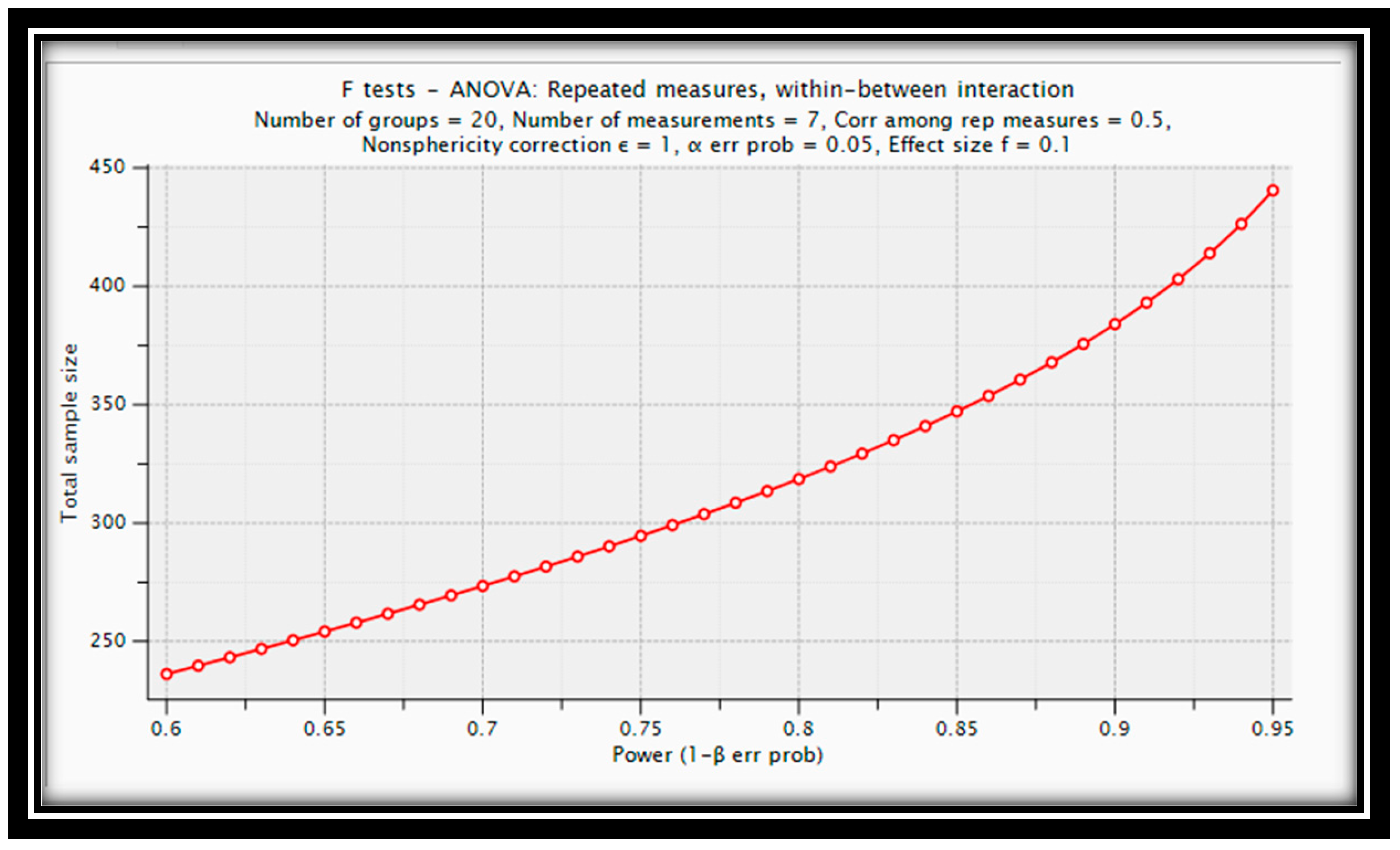
Table 1.
Description of Literature.
| Authors | Sample Size | Subject Used for Clustering | Compare Method | Compared Algorithm | Result |
|
Rodriguez et al. 2019 |
400 | Artificial datasets | distances between classes and correlations between features and average of the best accuracies | hierarchical, Clara, k-means, spectral, hc model, subspace, optics, DBSCAN, EM | Spectral algorithm consistently provided best performance for datasets with 10+ feature |
|
Hening 2021 |
35043 sample | Different categories (images, Texts, digits) there is large variation between the data sets | Just compare output of software | K-means, (Clara), (m-clust), (em-skew), (teigen), Single linkage hierarchical clustering, Average linkage hierarchical clustering, Complete linkage hierarchical clustering, Spectral clustering | “ The Gaussian mixture is the best for the largest amount of data. Differences between the other methods are not that pronounced, and all of them did best in some data sets.” |
|
Kaya And Schoop 2022 |
Ten negotiation experiments of several hundred participants with a total of 7026 exchanged negotiation interactions | Negotiation Support Systems (text) |
Principal Component Analysis | K-means, X-means, DBSCAN agglomerative |
With internal index k-Means and with external index k-Means or DBSCAN, performance is better. |
|
Costa et al 2023 |
n = 100 low, 600 moderates and 1000 |
Normal Mixed-type data | ANOVA-ARI-AMI-Effect size η2 | KAMILA, FAMD/K-Means, K-Prototypes, M-S K-Means, Mixed RKM, HL/PAM, Mixed K-Means, Gower/PAM | KAMILA, K-Prototypes and sequential Factor Analysis and K-Means clustering typically performed better than other methods |
|
Sepin et al 2024 |
data1:512 data2: ambiguous data3: ambiguous |
vibration data |
1 Arithmetic mean of absolute values (Abs Mean). 2Median of absolute values (Abs Median). 3 Standard deviation (Std). 4 Interquartile range (IQR). 5 Skewness of absolute values (Abs Skew). 6 Kurtosis of absolute values (Abs Kurt) | K-means, Gaussian Mixture Model, OPTICS | K-means outperformed GMM slightly, whereas OPTICS performed significantly worse. |
Table 2.
Software Libraries.
| Data Mining Platform | Rapid Miner | Weka |
| Algorithms Compared | K-Mean, K-Mean (H2O), K-Mean Kernal, K-Mean fast, X-Mean, K-Medoids, Fuzzy C-mean, Agglomerative Clustering, DBSCAN, Top-Down Clustering, Flatten Clustering, G-Means, Random | BANG-File, Canopy, Cascade Simple K-Mean, Cobweb, farthest first, Gen-Clust plus plus, Hierarchical Clustering, LVQ, EM, make density-based Clustering, OPTICS, SOM, sIB, , X-means |
Disclaimer/Publisher’s Note: The statements, opinions and data contained in all publications are solely those of the individual author(s) and contributor(s) and not of MDPI and/or the editor(s). MDPI and/or the editor(s) disclaim responsibility for any injury to people or property resulting from any ideas, methods, instructions or products referred to in the content. |
© 2025 by the authors. Licensee MDPI, Basel, Switzerland. This article is an open access article distributed under the terms and conditions of the Creative Commons Attribution (CC BY) license (http://creativecommons.org/licenses/by/4.0/).
Copyright: This open access article is published under a Creative Commons CC BY 4.0 license, which permit the free download, distribution, and reuse, provided that the author and preprint are cited in any reuse.


