
Submitted:
22 July 2025
Posted:
24 July 2025
You are already at the latest version
Abstract
The Pythagorean Expectation can be used to calculate expected winning percentage in various sports. This metric was developed by baseball statistician Bill James and has since been adapted in many sports, including cricket. The present study focuses on the application of the Pythagorean Expectation to derive winning percentages in women’s limited-over cricket. The traditional method of calculating a team’s winning percentage in cricket does not account for the margin of victory, defined as the difference between runs scored and runs allowed in a match. The Pythagorean Expectation takes into account both runs allowed and runs scored to provide a better representation of a team’s strength over a period of time in terms of the offensive and defensive output of a team. Eight women’s cricket teams of the International Cricket Council (ICC) were chosen for the study for two limited-over cricket formats -Twenty20 (T20) and One Day International (ODI).
Keywords:
women’s cricket
; Pythagorean formula
; runs allowed
; runs scored
; winning percentage
; maximum likelihood
; goodness of fit
1. Introduction
The Pythagorean Expectation is a sports analytics tool developed by statistician Bill James in the early 1980s. Initially the metric was used to measure a team’s performance over a season in baseball. The formula is now widely used in different sports to estimate the expected winning percentage of a team based on the number of points or runs they have scored and runs allowed. In bat and ball games like baseball and cricket, runs scored is defined as the number of runs a team accumulates while batting, and runs allowed refers to the total number of runs a team concedes while bowling. The metric derives its name from the renowned Pythagorean Theorem in geometry, as both involve calculations based on an exponent of 2. The traditional method of calculating a team’s winning percentage is by using the formula (Total Wins * 100 / Number of Matches). This method overlooks the margin of victory, defined as the difference between runs scored and runs allowed in a match. As a result, the traditional winning percentage may not accurately represent a team’s overall performance. The formula proposed by Bill James (McGrath, B., 2003) to compute the expected winning percentage is:
where RS indicates runs scored by the team and RA indicates runs allowed by the team respectively. A theoretical justification of the formula was given by Miller (2007). The original value of the γ, where γ is the exponent which gives us the best estimate for winning percentage, was computed as 2 in the formula given by Bill James for baseball. This metric takes into account runs allowed and runs scored to provide insight into whether a team’s win-loss record accurately reflects its overall performance or if it has been influenced by luck and other external factors giving a better idea regarding the offensive and defensive output of a team.
Cricket is widely recognized as a British sport which originated in the South-Eastern Counties of England in 1589. The British Empire exported cricket to its colonies in a bid to ‘civilize’ the native people. The first international cricket match was played in 1884 between the United States of America and Canada (Swanton, 1968). Women’s cricket itself has a rich history, with the first game played between village of Bramley and Hambledon on 15 August 1745, and the first ever Cricket World Cup was also played by women in 1973 (Threlfall-Sykes, 2015). Currently, cricket is played in three formats – Test, Twenty20 (T20) and One Day International (ODI). Although women do not play Test cricket on a regular basis, all three formats are played by both women and men. The T20 and the ODI formats have a fixed number of overs in a match, hence they are named limited over cricket.
The objective of this paper is to analyze the performance of a team in Women’s Limited Over Cricket based on computation of their expected winning percentages by using estimated values of the Pythagorean Exponent. This paper uses the Pythagorean Expectation to derive the expected winning percentages for women’s cricket teams of eight countries. The estimate of the appropriate Pythagorean Exponent is obtained by assuming that the runs allowed and the runs scored by a team follow a Weibull distribution (Hasika 2021). This estimate is then used to calculate the expected winning percentage of the selected women’s teams of the International Cricket Council (ICC) for the two limited –over cricket formats T20 and ODI. While previous studies have applied the Pythagorean Exponent to calculate winning percentages in men’s limited-over cricket, no research on its application in women’s limited-over cricket could be identified so far.
2. Applications of Pythagorean Expectation in various sports: A Brief Review
Initially, the work by Bill James was overlooked by most stakeholders in baseball. Over time it was recognized that using statistical measures like Pythagorean Expectation helped in understanding and analyzing a team’s performance in a better way. The Pythagorean Expectation has now been adapted for various other sports, including basketball, football, and hockey, with adjustments made to suit the specific scoring patterns of these games. It is a useful metric in forecasting future performance of a team by highlighting overperforming or underperforming teams. Teams can also use this metric to identify areas needing improvement in their games, such as offense or defense.
As the usage of this method became more widespread, statisticians and researchers have refined the formula to obtain a value of the exponent that fit the data better for different sports. Schatz (2003) applied it to determine the value of γ for the National Football League (NFL) and stated in his paper that it is applicable across all major sports. Oliver (2004) applied it to basketball and determined the Pythagorean Exponent to be 13.91. Dayaratna and Miller (2012) extended the metric for National Football League (NFL). They computed the exponent as 2.37 for the National Hockey League (NHL). Howard (2011) applied it to football and found the exponent value to be 1.7. Applications of the Pythagorean Exponent can be found in many studies related to the game of cricket. Perera and Swartz (2013), Vine (2016) and Senevirathne and Manage (2021) have analyzed this metric with respect to limited over cricket. Recent theoretical contribution to this formula is by Almeida et. al. (2025) who have derived the winning percentage by assuming that the runs allowed and runs scored follow Weibull distribution with different shape parameters.
3. Data Description
Each team in the game of cricket has two resources while batting, wickets in hand and balls remaining. In T20 format, each side is allowed to bat for 20 overs respectively. In ODI format, each side is allowed to bat for 50 overs, respectively, though it was 60 overs initially when ODI was started. Since ODI has a higher number of balls than T20, wickets become a more precise resource, so the batsmen need to give more importance to wicket preservation in ODI as compared to a T20 game. The chasing team’s innings gets over if they outscore their opponents, meaning that they are unable to use 100% of the resources allocated to them most of the time, or the entire team gets out before reaching the targeted score. Cricket, unlike many other sports cannot be played during rain, so the game is brought to a halt and several overs are deducted from a normal number of overs to compensate for the time lost due to rain. This leads to a shift in the distribution of available resources with a team. The Duckworth Lewis (DLS) Table (Duckworth and Lewis, 1998) is used to revise the target according to the number of overs lost. This method is officially used by ICC, the governing body of the game. The DLS Table is a mathematical table that provides the percentage of resources left with the team given that they have played x number of balls and lost y number of wickets.
For deriving the value of the Pythagorean Exponent, 12 teams were considered for the analysis. The teams from India, Pakistan, Sri Lanka, Australia, England, New Zealand, West Indies and South Africa were chosen for the study based on the consideration that these were the only teams that played cricket regularly between 2008 and 2024. The paper considers matches played between these teams during the specified timeframe. A total of 376 and 320 matches of T20 and ODI format, respectively, played by these teams were included for the analysis. The matches were played between 2009 to 2024 for T20I and 2007 to 2024 for the ODI format. Traditionally, the 12 teams have a rich cricketing history, although primarily in men’s category, which meant that basic infrastructure for the game was available for the players. Any match interrupted by rain or overs lost due to any reason, was not considered for the study. Data has been obtained from an open source cricket data website, cricsheet.org. The cleaning and analysis of data was done using Python, Excel and R.
Table 1 gives the descriptive statistics for the runs scored in T20 for all the teams after extrapolation using the DLS Table. The average score ranges from a minimum of 112 (Pakistan) to a high of 149 (Australia).The maximum runs scored by a team was 250 (England) and the minimum runs scored by a team was 46 (Sri Lanka).
Descriptive statistics for runs allowed in T20 matches are given in Table 2. The average score ranges from a minimum of 126 (England) to a high of 135 (India). The maximum runs scored by a team was 250 (South Africa) and the minimum runs scored by a team was 46 (South Africa). The minimum and maximum runs scored by a team and allowed by a team are same in the T20 format.
Winning percentages of the teams in the T20 match format are given in Table 3. Australia has the highest winning percentage of 75.23% amongst the teams, followed by England with the next best winning percentage of 71.54%. Sri Lanka and Pakistan have the lowest winning percentages at 23.19% and 29.07%, respectively.
Table 4 gives the descriptive statistics for the runs scored in the ODI format. The scores have been extrapolated, wherever necessary, using the DLS table. The average score ranges from a minimum of 179 (Sri Lanka) to a high of 254 (Australia). The maximum runs scored by a team in ODI matches was 378 (England) and the minimum runs scored by a team was 48 (West Indies).
Descriptive statistics for runs allowed in ODI matches are given in Table 5. The average score ranges from a minimum of 202 (Australia) to a high of 229 (Sri Lanka). The maximum runs scored by a team was 378 (Pakistan) and the minimum runs scored by a team was 48 (South Africa).
Winning percentages of the teams in the ODI format are given in Table 6. Australia has the highest winning percentage of 84.44% among the teams. England has the next best winning percentage at 64.71%. Pakistan and Sri Lanka have the lowest percentages amongst the teams selected.
4. Methodology
In the game of cricket, if a chasing team reaches the winning score before utilizing all their allocated overs, it indicates that they did not use 100% of their resources. This can lead to dependency between runs scored and runs allowed. For validation of the statistical methods and to take care of the dependency problem, Vine (2006) suggested a way out by extrapolating the runs scored by the chasing team using the DLS table. In this study, the DLS table was used to measure the percentage of resources left with the team and this was added to their team’s total. The study assumes that both teams utilized 100 percent of their resources during the match.
Based on the study by Miller (2007), the distribution of runs scored (RS) and runs allowed (RA) by the respective teams are assumed to follow independent Weibull distribution with a common shape parameter. The probability density function (pdf) of the three parameter Weibull Distribution with parameters (α, β, γ) is as follows:
where γ is the shape parameter, α is the scale parameter, and β is the location parameter of this distribution.
It is assumed that the runs scored in a match follow a Weibull distribution with parameters (), while the runs allowed in a match also follow a Weibull distribution with parameters (). Under these assumptions, it can be shown that,
where RS = and RA =
The winning percentage of a team,as proposed by Bill Smith,is then given by:
A complete derivation of this method can be found in Miller (2007). The present study uses the Maximum Likelihood Method introduced by Miller (2007) for estimation of parameters.
4.1. Data Analysis - Parameter Estimation
The Weibull distribution assumes continuous data, while the data recorded in cricket is discreet in nature. To convert the discreet data into continuous, the deliveries in the match are divided into bins.
For T20, the bins considered are -
[-0.5, 19.5] [19.5, 39.5] [39.5, 59.5] … [119.5,139.5] [159.5,∞].
For ODI the bins considered are-
[-0.5, 49.5] U [49.5, 99.5] U [99.5, 149.5] U…U [299.5, 349.5] U [349.5,∞].
The value of the parameter β is assumed to be – 0.5 based on the study by Senevirathne and Manage (2021) for men’s limited over cricket. For estimation of the parameters (initially three methods were considered - Maximum Likelihood Estimation (MLE), Method of Moments (MoM) and Method of Least Squares Estimation (LSE). Table 7 gives a comparison of the MSEs for all the methods. For T20 the method of LSE gave the best results for Mean Square Error (MSE) and for ODI MLE gave the best results. The goodness of fit test was better for both formats using the MLE method. So, keeping that in consideration, the MLE method was used for estimation of parameters for the data.
Subsequently, the winning percentage of each team was calculated using the formula,
Thereafter, the winning percentage was calculated for each team using the γ obtained for each team. Then a simple average was taken for the obtained values of γ, giving the desired value of γ.
Table 8 gives the values of γ for T20 matches of all the teams computed by maximum likelihood method. The value obtained for T20 matches is 5.09 with a standard deviation of 0.3. The sum of error term squared between predicted winning percentage and actual winning percentage is 199.75. The average difference between predicted wins and actual wins is -0.5 with a standard deviation of 5.29.
Table 9 gives the values of γ for ODI matches played by all the teams computed by the MLE method. The average value of γ obtained for ODI is 4.65 with a standard deviation of 0.94. The sum of error term squared between predicted winning percentage and actual winning percentage in this case is obtained as 231.59. The average difference between predicted wins and actual wins is 1.38 with a standard deviation of 4.14.
4.2. Goodness of Fit Tests
The Chi-square test for goodness of fit was applied to assess the suitability of the Weibull distribution in modeling runs scored and runs allowed for each team. The parameters αRS, αRA and γ, estimated by the maximum likelihood method for each team, respectively, were used for the goodness of fit test. The p-values for runs scored and runs allowed by each team in T20 and ODI matches are shown in Table 10 and Table 11, respectively. The goodness of fit plots for runs allowed and runs scored in ODIs for India are shown in Figure 1. The Appendix A contains the plots for all teams in both T20 and ODI matches.
Table 10 gives the p-values for runs scored and runs allowed in T20 matches. All the values for the runs scored model for T20 matches are above 0.05 except for West Indies. All values of runs allowed are above 0.05 for runs allowed except for Sri Lanka which is above 0.02. The p-values for runs scored and runs allowed for ODIs are given in Table 11. All the values for the runs allowed model for ODI matches are well above 0.05 with the only exception of Australia. Overall, the Weibull distribution can be considered a good fit to the data in both cases. For all the other teams, the goodness of fit plots are given in the Appendix A.
5. Discussion and Conclusions
In this study, the mean Pythagorean Exponent γ has been calculated as 4.65 for T20 and 5.09 for ODI formats in women’s international cricket. Ten teams were chosen for the study based on the frequency of matches they played between 2008 and 2024. The values of the Pythagorean Exponent for individual teams were higher for T20 matches as compared to ODI matches. A possible explanation could be the irregular scheduling of ODI matches in comparison to T20 matches. The winning percentages for all the teams were subsequently calculated for the two limited over cricket formats. The study identified Australia as the most dominant team in women’s international limited-over cricket in terms of winning percentages for both T20 and ODI formats with Sri Lanka and Pakistan being the least dominant teams respectively.
The Australian-women’s cricket team has won the ICC Women’s T20 World Cup six times, in the years 2010, 2012, 2014, 2018, 2020, and 2023.They also won the ICC Women’s Cricket World Cup a record seven times since 1973, the last win being in 2022. The England-women’s cricket team has won the ICC Women’s Cricket World Cup four times, the last one being the 2017 Women’s World Cup. Both these teams have won it twice during the period for which the study was conducted. Thus, the results of this study are consistent with the performances of these two teams. The present study examines runs scored and runs allowed by each team in matches played against each other. Further research could explore calculating the exponent based on specific team pairings and is suggested as a direction for future research.
Conflicts of Interest
The authors do not have any financial or non-financial conflict of interest to declare for the research work included in this article.
Appendix A
Figure A1.
Weibulldistribution fit for runs scored and runs allowed for Australia (ODI).
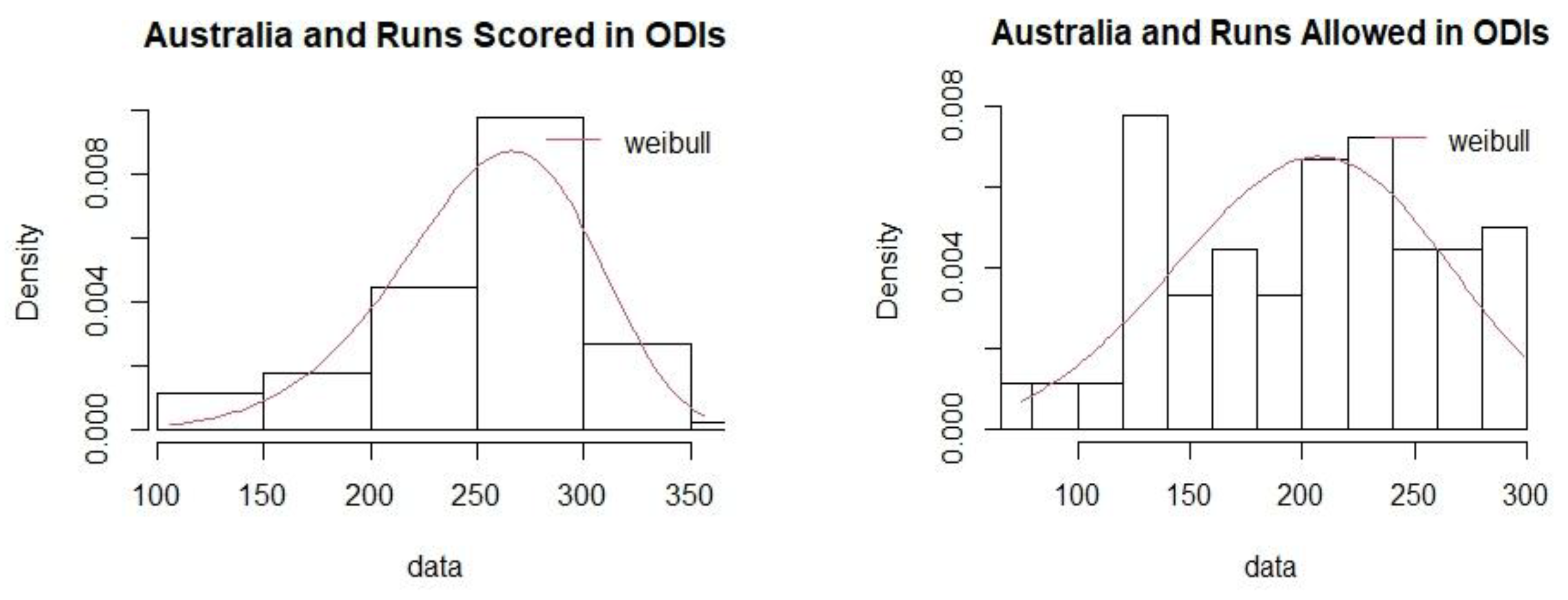
Figure A2.
Weibulldistribution fit for runs scored and runs allowed for England (ODI).
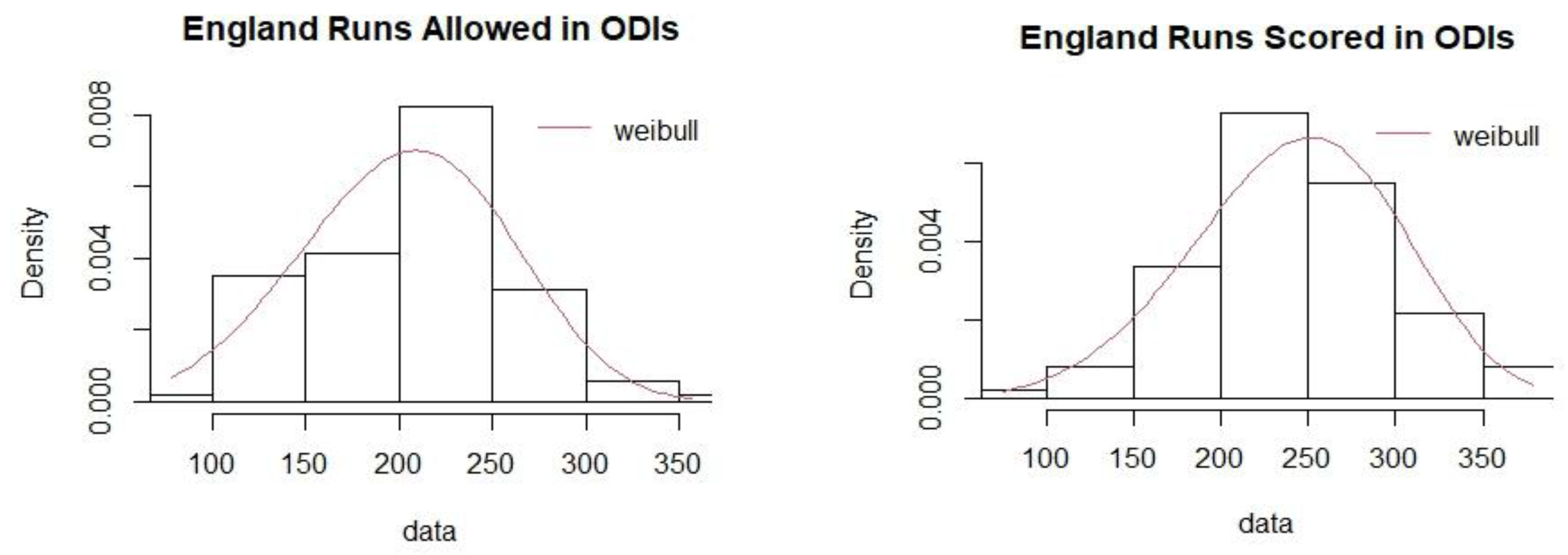
Figure A3.
Weibulldistribution fit for runs scored and runs allowed for New Zealand (ODI).
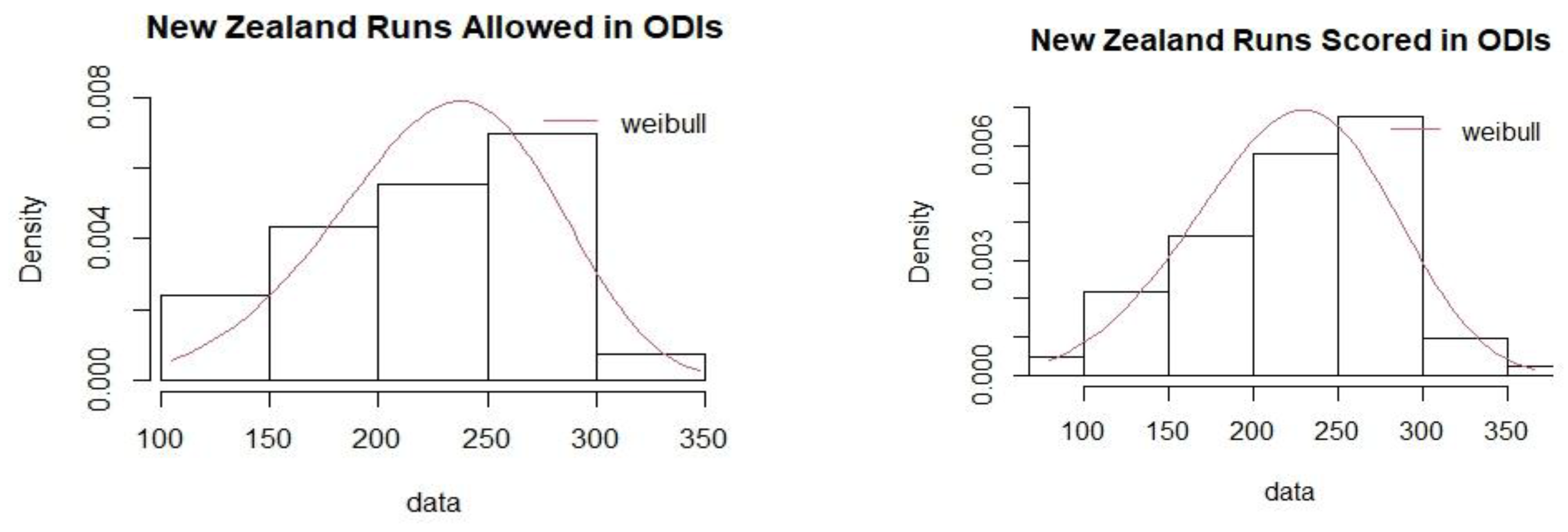
Figure A4.
Weibull distribution fit for runs scored and runs allowed for Pakistan (ODI).
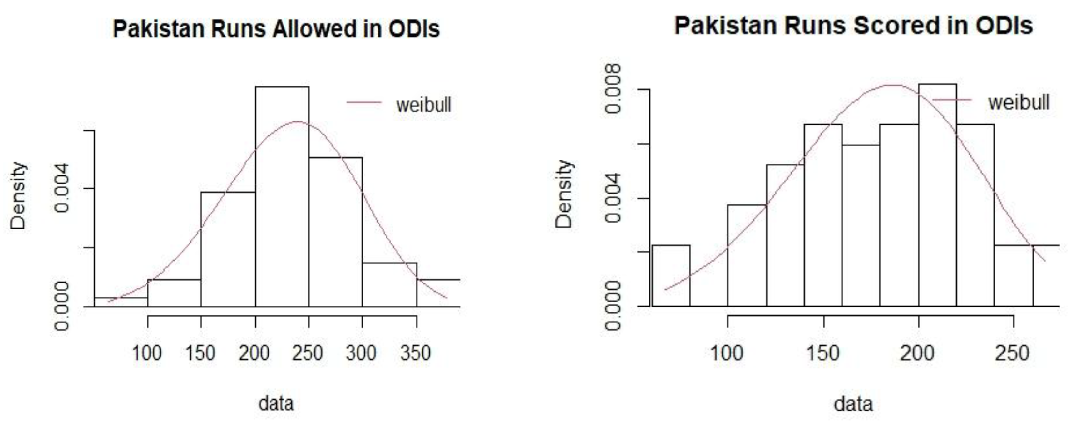
Figure A5.
Weibulldistribution fit for runs scored and runs allowed for South Africa (ODI).
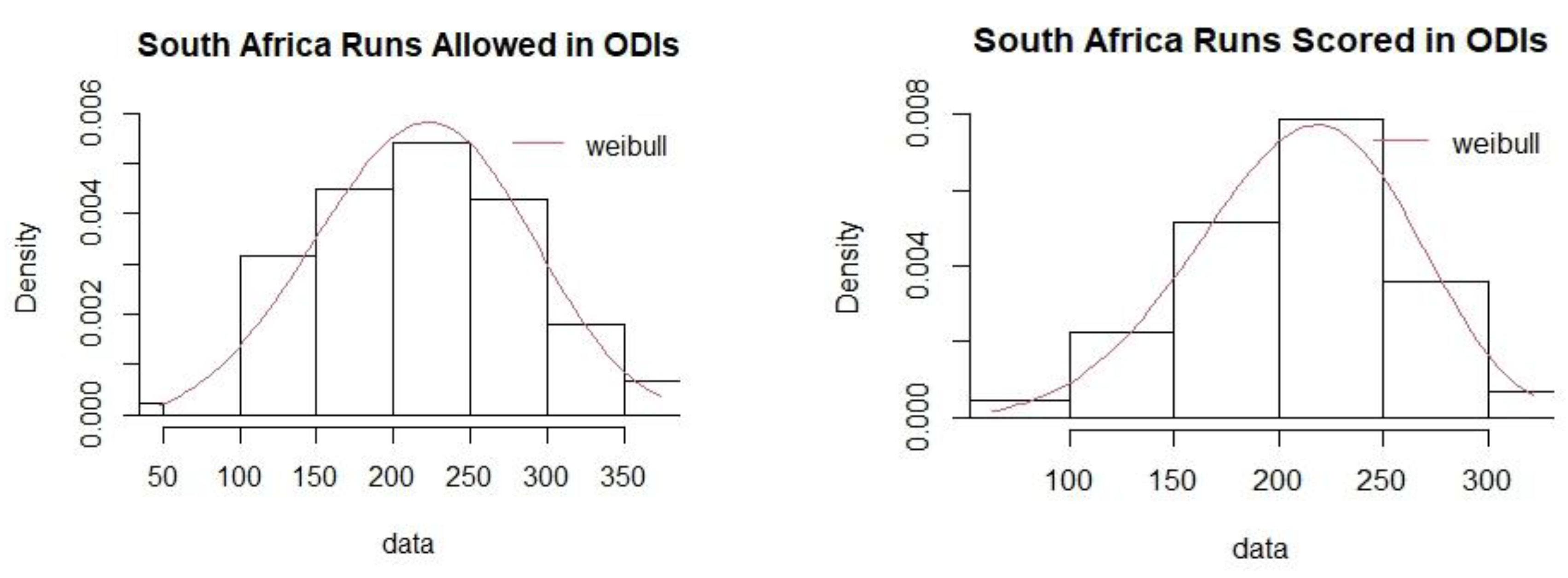
Figure A6.
Weibull distribution fit for runs scored and runs allowed for Sri Lanka (ODI).
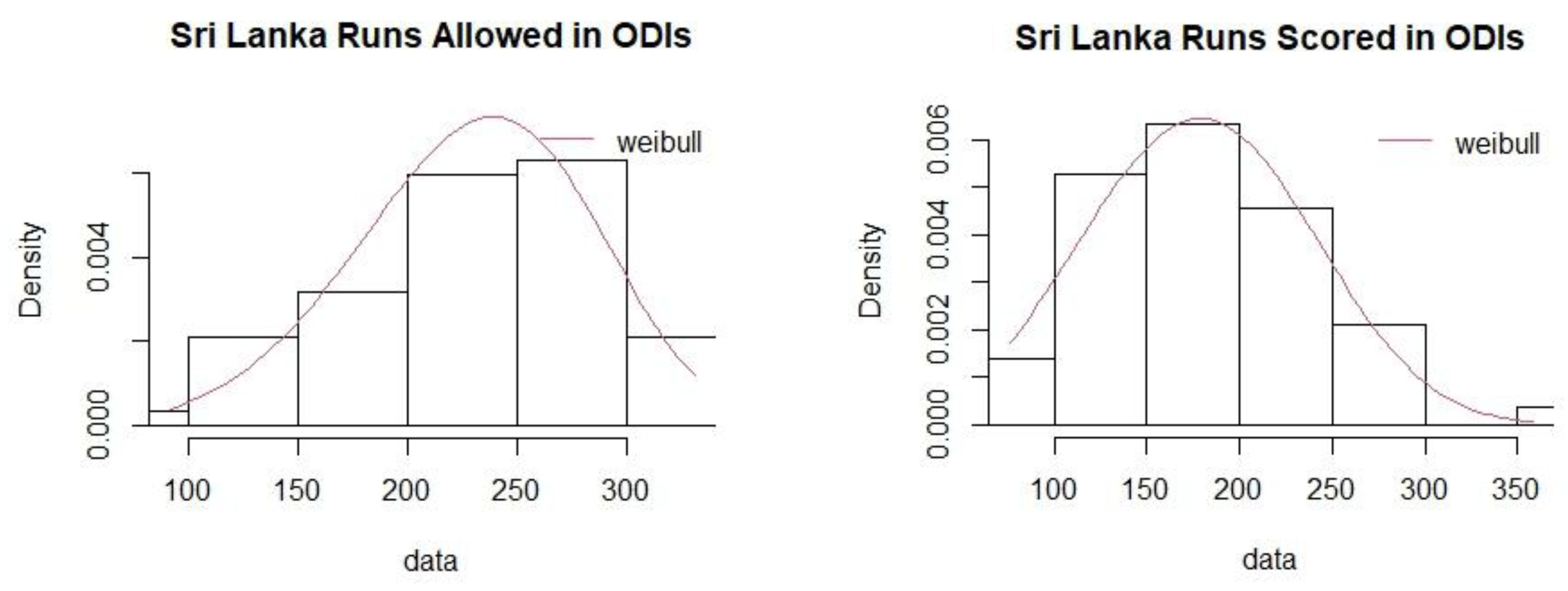
Figure A7.
Weibull distribution fit for runs scored and runs allowed for West Indies (ODI).
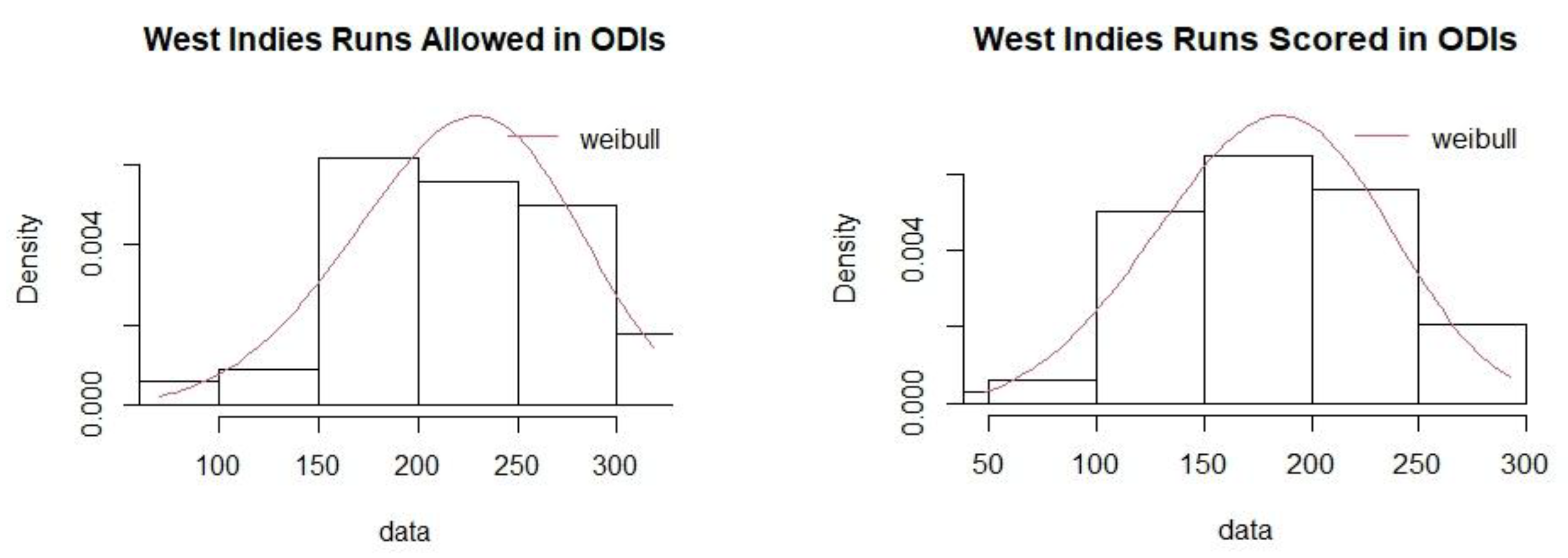
Figure A8.
Weibulldistribution fit for runs scored and runs allowed for India (T20I).
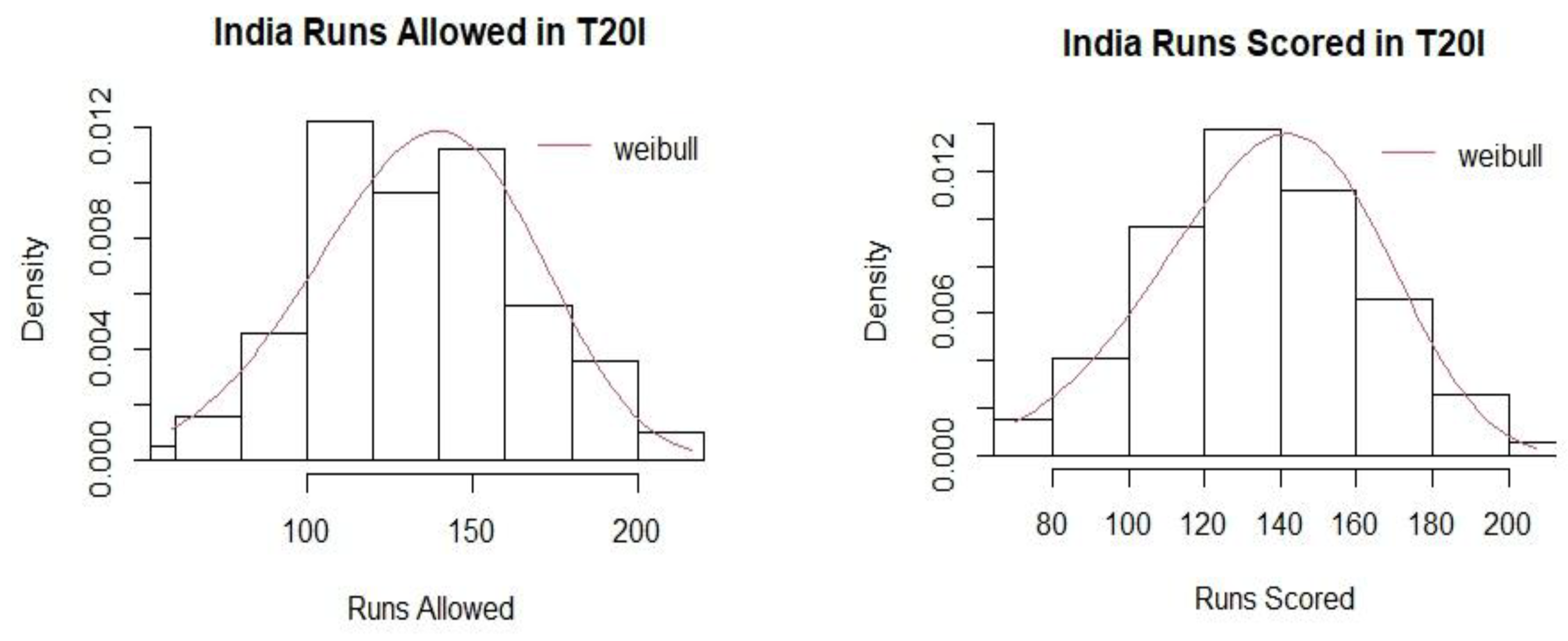
Figure A9.
Weibulldistribution fit for runs scored and runs allowed for Australia (T20I).
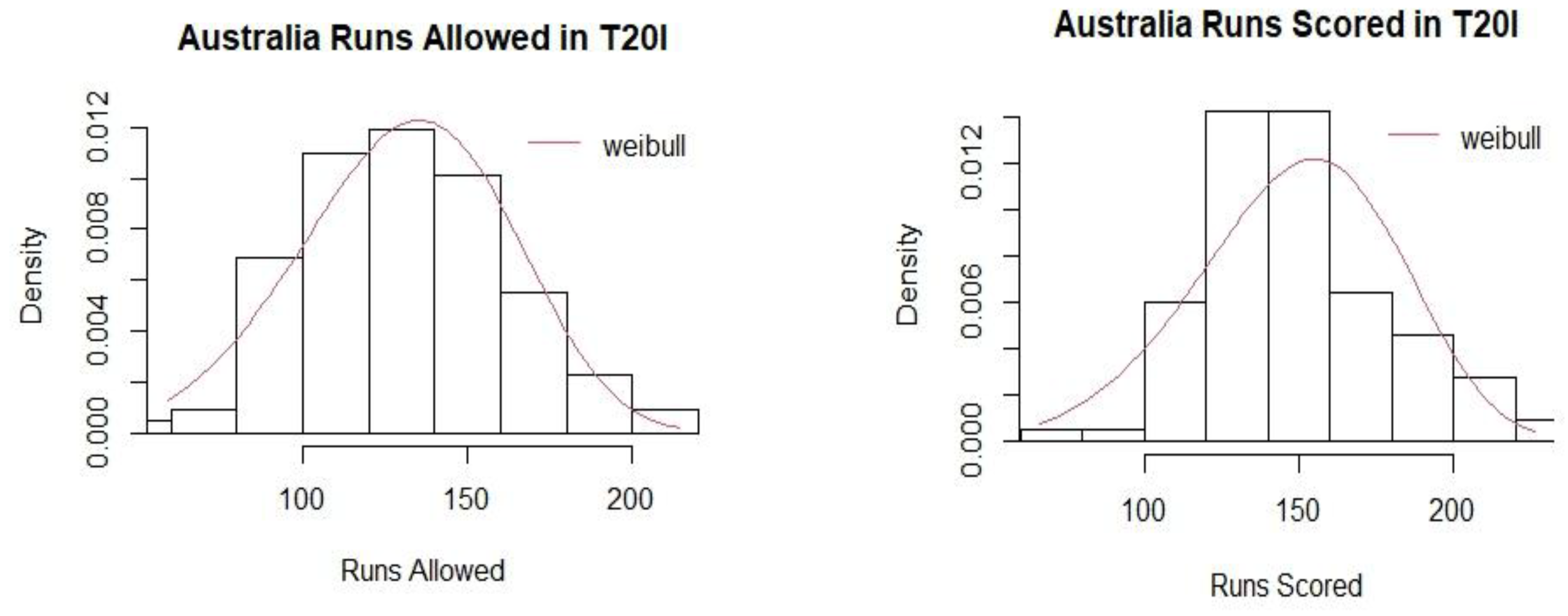
Figure A10.
Weibull Distribution Fit for Runs Scored and Runs Allowed for England (T20I).
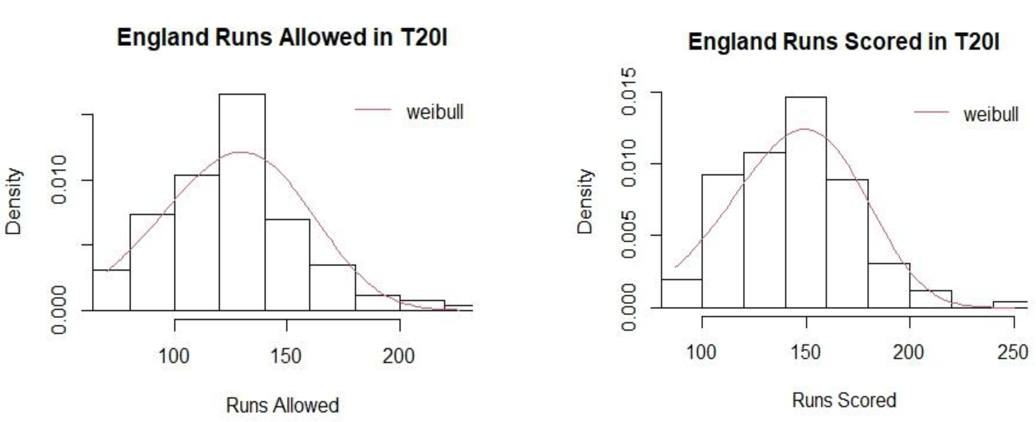
Figure A11.
Weibulldistribution fit for runs scored and runs allowed for New Zealand (T20I).
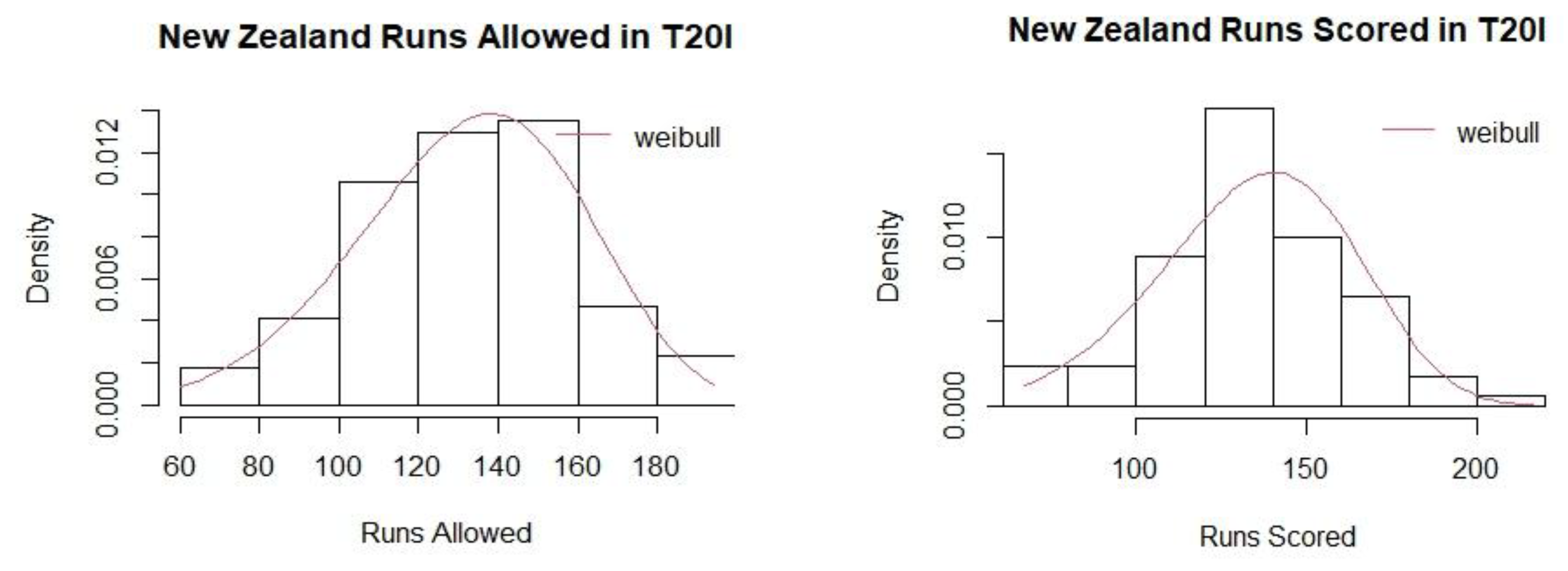
Figure A12.
Weibulldistribution fit for runs scored and runs allowed for Pakistan (T20I).
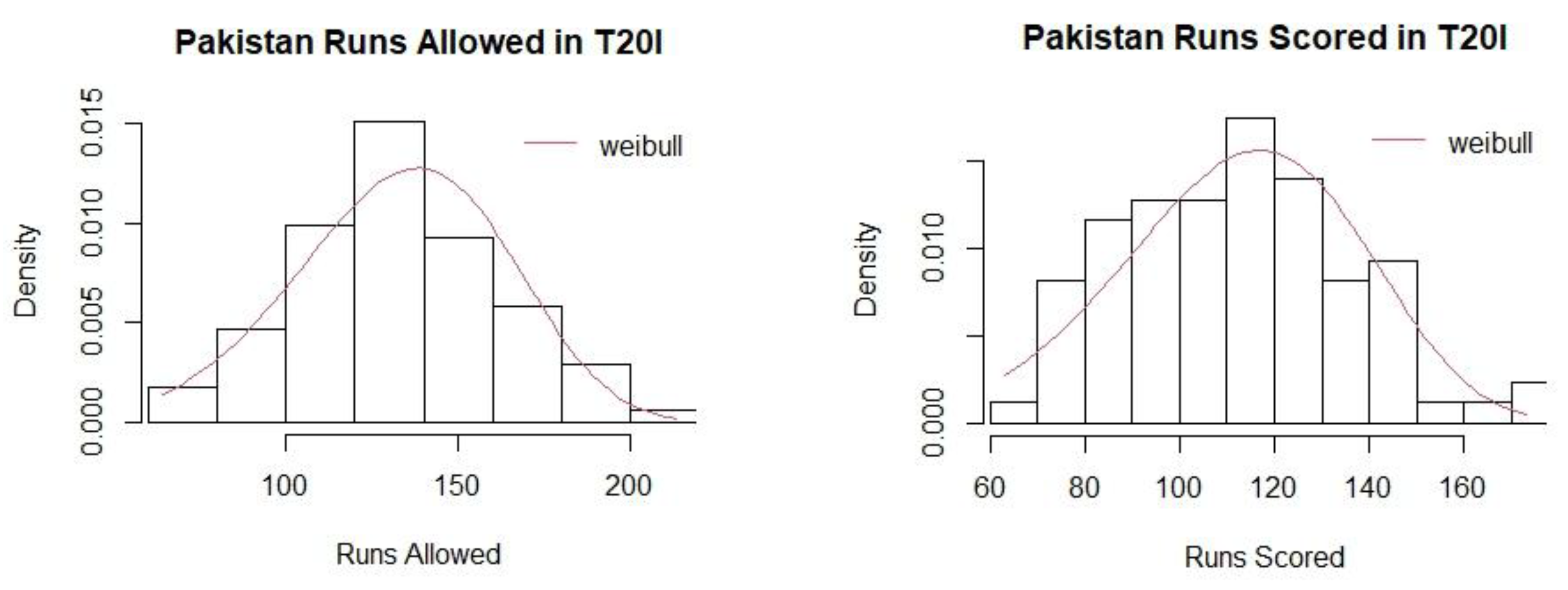
Figure A13.
Weibulldistribution fit for runs scored and runs allowed for South Africa (T20I).
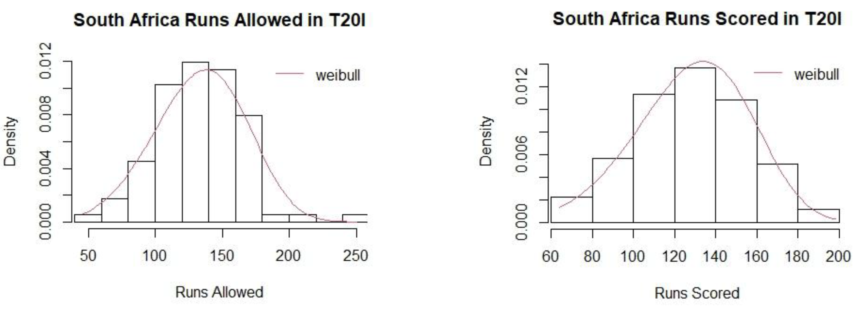
Figure A14.
Weibulldistribution fit for runs scored and runs allowed for Sri Lanka (T20I).
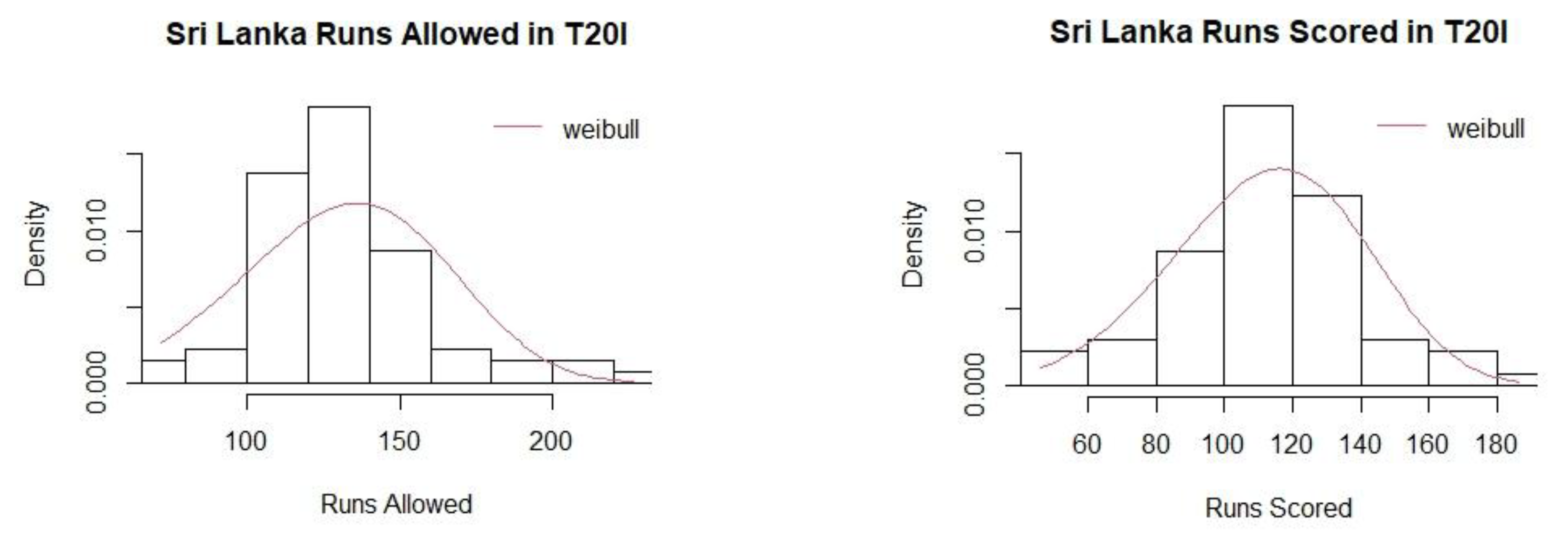
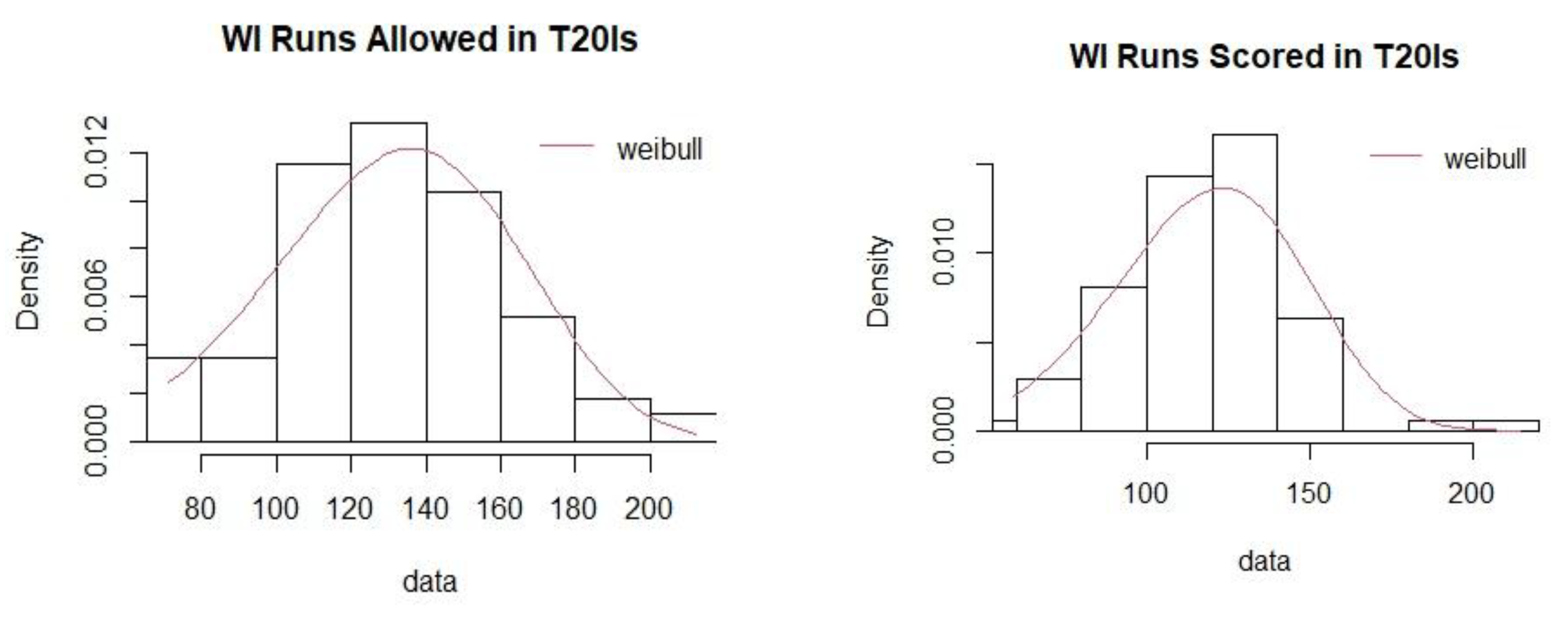
Figure A15.
Weibulldistribution fit for runs scored and runs allowed for West Indies (T20I).
References
- Almeida, A.F., Dayaratna, K., Miller, S.J., Yang, A.K. (2025). Applications of improvements to the Pythagorean won-lost expectation in optimizing rosters. In: Blondin, M.J., Fister Jr., I., Pardalos, P.M. (Eds.) Artificial Intelligence, Optimization, and Data Sciences in Sports. Springer Optimization and Its Applications, 218, Springer, Cham. [CrossRef]
- Caro, C. A. and Machtmes, R. (2013). Testing the utility of the Pythagorean Expectation formula on division one college football: An examination and comparison to the Morey model. Journal of Business & Economics Research (Online), 11, 537.
- Dayaratna, K.D. and Miller, S.J. The Pythagorean win-loss formula and hockey. The Hockey Research Journal, 2012; 16, 193–209. [Google Scholar]
- Duckworth, F.C. and Lewis, A.J. (1998). A fair method for resetting the target in interrupted one-day cricket matches. Journal ofthe Operational Research Society, 49, 220–227.
- Hamilton, H. H. (2011). An extension of the Pythagorean Expectation for association football. Journal of Quantitative Analysis in Sports, 7, 15.
- McGrath, B. (2003). The professor of baseball. The New Yorker, 79, 038–038.
- Miller, S.J. (2007). A derivation of the Pythagorean won-loss formulabaseball. Chance, 20, 40–48. [CrossRef]
- Oliver, D. (2004). Basketball on Paper: Rules and Tools for Performance Analysis, University of Nebraska Press.
- Perera, H. P. and Swartz, T.B. (2013). Resource estimation in T20 cricket. IMA Journal of Management Mathematics 24, 337–347. [CrossRef]
- Schatz, A. (2003). Pythagoras on the Gridiron. Football Outsiders, 14.
- Senevirathne, H. K. and Manage, A. B. (2021). Predicting the winning percentage of limited-overs cricket using the Pythagorean formula. Journal of Sports Analytics, 7, 169–183.
- Swanton, H.A. A History of Cricket, Vol I.Unwin & Allen. 1968. [Google Scholar]
- Threlfall-Sykes, J. (2015). A History of English Women’s Cricket, 1880–1939.
- Vine, A. J. (2016). Using Pythagorean Expectation to determine luck in the KFC big bash league. Economic Papers: A Journal of Applied Economics and Policy, 35, 269–281.
Figure 1.
Goodness of fit plots for runs scored and runs allowed for India (ODI).
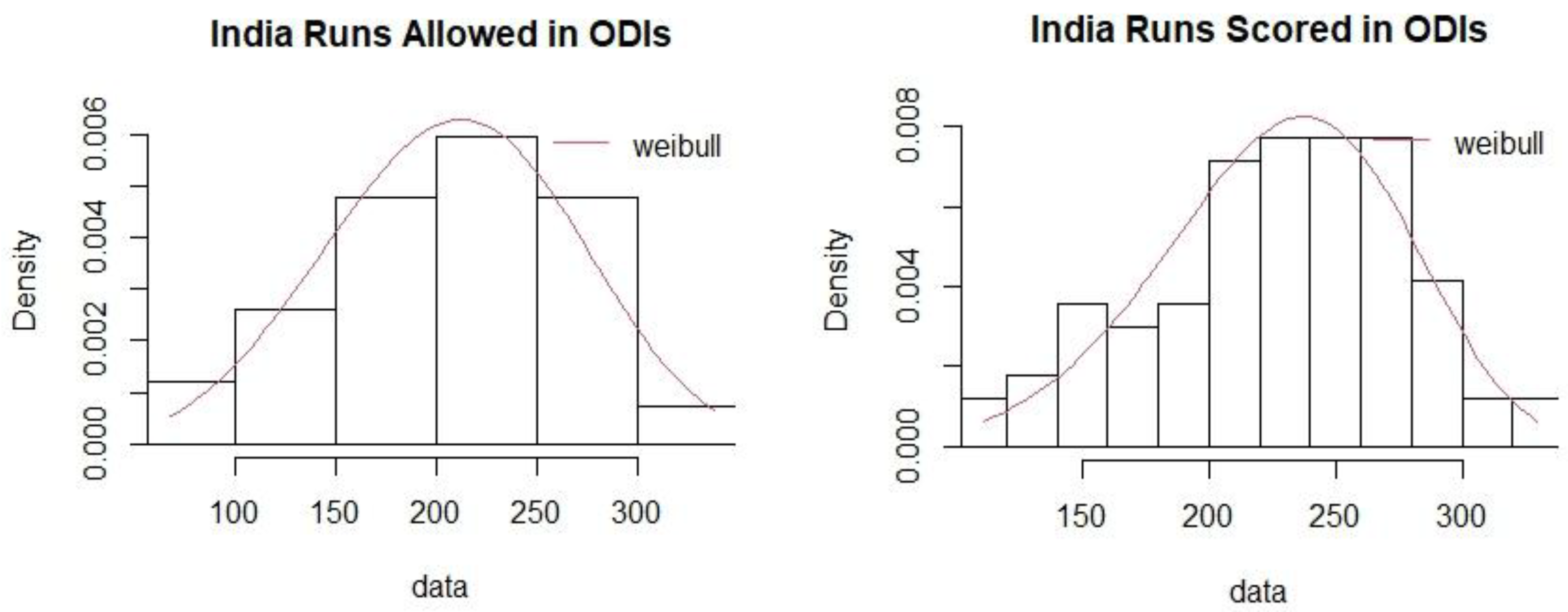

Table 1.
Descriptive statistics for runs scored in T20 matches.
| Teams | Average | Minimum | 1 Quartile | Median | 3 Quartile | Maximum |
|---|---|---|---|---|---|---|
| India | 136 | 70 | 116 | 136 | 155 | 207 |
| Australia | 149 | 66 | 128 | 147 | 163 | 226 |
| England | 144 | 87 | 123 | 145 | 162 | 250 |
| New Zealand | 135 | 67 | 118 | 133 | 151 | 216 |
| West Indies | 122 | 70 | 107 | 122 | 138 | 214 |
| South Africa | 128 | 64 | 112 | 130 | 149 | 198 |
| Pakistan | 112 | 63 | 95 | 113 | 126 | 173 |
| Sri Lanka | 113 | 46 | 99 | 111 | 127 | 186 |
Table 2.
Data description of runs allowed in T20 matches.
| Teams | Average | Minimum | 1 Quartile | Median | 3 Quartile | Maximum |
|---|---|---|---|---|---|---|
| India | 135 | 59 | 112 | 134 | 159 | 216 |
| Australia | 131 | 59 | 106 | 129 | 151 | 214 |
| England | 126 | 70 | 106 | 127 | 141 | 226 |
| New Zealand | 132 | 60 | 110 | 133 | 152 | 194 |
| West Indies | 131 | 71 | 111 | 131 | 150 | 212 |
| South Africa | 134 | 46 | 115 | 131 | 155 | 250 |
| Pakistan | 133 | 64 | 113 | 133 | 152 | 213 |
| Sri Lanka | 132 | 72 | 115 | 128 | 145 | 226 |
Table 3.
Winning percentage for teams in T20 matches.
| Team | No. of Wins | No. of Matches | Winning Percentage |
|---|---|---|---|
| India | 46 | 98 | 46.94 |
| Australia | 82 | 109 | 75.23 |
| West Indies | 34 | 87 | 39.08 |
| England | 93 | 130 | 71.54 |
| Sri Lanka | 16 | 69 | 23.19 |
| Pakistan | 25 | 86 | 29.07 |
| South Africa | 36 | 88 | 40.91 |
| New Zealand | 44 | 85 | 51.76 |
Table 4.
Descriptive statistics for runs scored in ODI matches.
| Teams | Average | Minimum | 1 Quartile | Median | 3 Quartile | Maximum |
|---|---|---|---|---|---|---|
| India | 227 | 111 | 200 | 234 | 265 | 329 |
| Australia | 254 | 106 | 231 | 265 | 282 | 356 |
| England | 242 | 75 | 210 | 241 | 281 | 378 |
| New Zealand | 221 | 79 | 179 | 230 | 258 | 365 |
| West Indies | 181 | 48 | 147 | 182 | 215 | 292 |
| South Africa | 210 | 63 | 181 | 215 | 244 | 321 |
| Pakistan | 180 | 67 | 146 | 189 | 216 | 266 |
| Sri Lanka | 179 | 76 | 134 | 173 | 216 | 358 |
Table 5.
Data description for runs allowed in ODI matches.
| Teams | Average | Minimum | 1 Quartile | Median | 3 Quartile | Maximum |
|---|---|---|---|---|---|---|
| India | 207 | 67 | 161 | 216 | 258 | 338 |
| Australia | 202 | 75 | 148 | 210 | 255 | 298 |
| England | 203 | 78 | 165 | 206 | 240 | 356 |
| New Zealand | 227 | 105 | 194 | 235 | 266 | 347 |
| West Indies | 221 | 70 | 186 | 221 | 259 | 318 |
| South Africa | 219 | 48 | 161 | 220 | 265 | 373 |
| Pakistan | 232 | 63 | 201 | 233 | 267 | 378 |
| Sri Lanka | 229 | 92 | 195 | 238 | 268 | 331 |
Table 6.
Winning percentage for teams in ODI matches.
| Team | No. of Wins | No. of Matches | Winning Percentage |
|---|---|---|---|
| South Africa | 46 | 89 | 51.69 |
| Pakistan | 14 | 67 | 20.9 |
| New Zealand | 33 | 83 | 39.76 |
| Sri Lanka | 12 | 57 | 21.05 |
| India | 51 | 84 | 60.71 |
| Australia | 76 | 90 | 84.44 |
| West Indies | 22 | 68 | 32.35 |
| England | 66 | 102 | 64.71 |
Table 7.
Comparison of MSE for different methods of estimation.
| ODI | T20 | |||||
|---|---|---|---|---|---|---|
| Teams | Square Error using MLE | Square Error using MoM | Square Error using LSE | Square Error using MLE | Square Error using MoM | Square Error using LSE |
| India | 1.06 | 0.47 | 0.33 | 17.22 | 10.69 | 10.76 |
| Australia | 6.5 | 13.67 | 23.55 | 97.22 | 39.98 | 28.64 |
| West Indies | 0.55 | 0.39 | 0.23 | 1.51 | 2.32 | 4.5 |
| England | 23.43 | 29.46 | 30.04 | 44.22 | 14.9 | 5.88 |
| Sri Lanka | 28.94 | 26.62 | 18.95 | 27.04 | 37.11 | 33.82 |
| Pakistan | 7.67 | 10.82 | 12.97 | 0.49 | 0.02 | 1.28 |
| South Africa | 31.7 | 30.89 | 29.39 | 10.24 | 2.14 | 1.57 |
Table 8.
The value of γ for T20 matches.
| Teams | No. of Games | Observed Wins | Observed Percentage | Predicted Percentage | Predicted Wins | Game Diff | γ |
|---|---|---|---|---|---|---|---|
| India | 98 | 46 | 46.94 | 51.17 | 50.15 | 4.15 | 5.34 |
| Australia | 109 | 82 | 75.23 | 66.18 | 72.14 | -9.86 | 5.21 |
| West Indies | 87 | 34 | 39.08 | 37.66 | 32.77 | -1.23 | 4.69 |
| England | 130 | 93 | 71.54 | 66.42 | 86.35 | -6.65 | 5.14 |
| Sri Lanka | 69 | 16 | 23.19 | 30.72 | 21.2 | 5.2 | 4.57 |
| Pakistan | 86 | 25 | 29.07 | 29.88 | 25.7 | 0.7 | 5.06 |
| South Africa | 88 | 36 | 40.91 | 44.54 | 39.2 | 3.2 | 5.29 |
| New Zealand | 85 | 44 | 51.76 | 52.27 | 44.43 | 0.43 | 5.38 |
Table 9.
The value of γ for ODI matches.
| Teams | No. of Games | Observed Wins | Observed Percentage | Predicted Percentage | Predicted Wins | Game Diff | γ |
|---|---|---|---|---|---|---|---|
| India | 84 | 51 | 60.71 | 61.93 | 52.03 | 1.03 | 5.43 |
| Australia | 90 | 76 | 84.44 | 81.06 | 73.45 | -2.55 | 6.4 |
| West Indies | 68 | 22 | 32.35 | 31.25 | 21.26 | -.74 | 3.94 |
| England | 102 | 66 | 64.70 | 69.45 | 70.84 | 4.84 | 4.65 |
| Sri Lanka | 57 | 12 | 21.05 | 30.48 | 17.38 | 5.38 | 3.31 |
| Pakistan | 67 | 14 | 20.89 | 25.02 | 16.77 | 2.77 | 4.27 |
| South Africa | 89 | 46 | 51.68 | 45.35 | 40.37 | -5.63 | 4.7 |
| New Zealand | 83 | 33 | 39.75 | 46.98 | 38.99 | 5.99 | 4.43 |
Table 10.
p-values for Goodness of Fit tests for T20 matches.
| Team | Runs Scored p-value | Runs Allowed p-value |
|---|---|---|
| India | 0.9886 | 0.7578 |
| Australia | 0.1359 | 0.8180 |
| England | 0.5784 | 0.1710 |
| South Africa | 0.9982 | 0.8070 |
| Pakistan | 0.8968 | 0.9780 |
| Sri Lanka | 0.4641 | 0.0295 |
| New Zealand | 0.6422 | 0.9901 |
| West Indies | 0.0008 | 0.6391 |
Table 11.
p-values for Goodness of Fit tests for ODI matches.
| Team | Runs Scored p-value | Runs Allowed p-value |
|---|---|---|
| South Africa | 0.9486 | 0.4788 |
| India | 0.4816 | 0.8760 |
| England | 0.7767 | 0.0746 |
| Australia | 0.2085 | 0.0072 |
| New Zealand | 0.4982 | 0.3765 |
| Pakistan | 0.9325 | 0.5531 |
| Sri Lanka | 0.1090 | 0.7854 |
| West Indies | 0.8019 | 0.5650 |
Disclaimer/Publisher’s Note: The statements, opinions and data contained in all publications are solely those of the individual author(s) and contributor(s) and not of MDPI and/or the editor(s). MDPI and/or the editor(s) disclaim responsibility for any injury to people or property resulting from any ideas, methods, instructions or products referred to in the content. |
© 2025 by the authors. Licensee MDPI, Basel, Switzerland. This article is an open access article distributed under the terms and conditions of the Creative Commons Attribution (CC BY) license (http://creativecommons.org/licenses/by/4.0/).
Copyright: This open access article is published under a Creative Commons CC BY 4.0 license, which permit the free download, distribution, and reuse, provided that the author and preprint are cited in any reuse.


