Submitted:
23 July 2025
Posted:
24 July 2025
You are already at the latest version
Abstract
Accurate color property measurements are critical for advancing artificial vision in re-al-time industrial applications. RGB imaging remains highly applicable and widely used due to its practicality, accessibility, and high spatial resolution. However, significant un-certainties in extracting chromatic information highlight the need to define when conven-tional digital images can reliably provide accurate color data. This work simultaneously compares six chromatic properties across 700 Pantone® TCX fabric samples, using opti-cal data acquired simultaneously from both hyperspectral (HSI) and digital (RGB) camer-as. The results indicate that the accurate interpretation of optical information from RGB (sRGB and REC2020) images is significantly influenced by lightness (L*) values. Samples with bright and unsaturated colors (L* > 50) reach ratio-to-performance-deviation (RPD) values above 2.5 for four properties (L*, a*, b* H), indicating a high correlation between HSI and RGB information. Direct color difference comparisons (∆E) between HSI and RGB images yield values exceeding 5.5 for red-yellow-green samples and up to 9.0 for blue and purple tones. However, when relative color differences (∆E′) are calculated using a specific reference, the values drop significantly falling below 2.0 for light-colored samples (L* > 50). These results confirm that RGB imagery achieves reliable color consistency when evalu-ated against a practical reference.

Keywords:
hyperspectral imaging
; sRGB-REC2020 images
; CIE-L*a*b* color space
; relative color differences
1. Introduction
In Color appearance is a primary sensory attribute commonly linked to the quality, purity, and chemical composition of an object. Rather than representing intrinsic properties of a sample, color reflects the visual response arising from its optical characteristics interacting with an illumination source [1,2,3,4]. Important processes in industries such as automotive, textile, food, pharmaceutical, cosmetic, and packaging require thorough color inspection for tasks such as painting matching, fabric dyeing, garment color consistency, ensuring food and beverage quality, medication identification and quality, hair dye formulation, makeup consistency, and packaging design [5,6]. These processes are crucial for enhancing product appeal, preserving brand consistency, and ensuring consumer satisfaction. However, color evaluation has traditionally relied on visual inspection by trained personnel, whose assessments may vary due to factors such as lighting conditions, individual perceptual differences, and visual fatigue—introducing inherent ambiguities and inconsistencies [7,8].
In recent decades, advancements in artificial and computer vision, driven primarily by image and video processing technologies alongside the development of sophisticated algorithms and software, have enabled the automation of analysis protocols for identification, classification, and real-time assessment in industries such as pharmaceuticals [9,10], food [11,12], and textiles[13], among others, throughout production and processing stages. For instance, in agricultural implementation Rodriguez-Pulido et al. developed an application that facilitates the integration of color and NIR spectral information, enabling simultaneous extraction at the pixel or object level. This study was applied to grape and grape seed samples in the individual evaluation of differences associated with the visible and NIR regions at the same time. Likewise, Machine-vision by assessing shape, size and color of strawberries has been developed using line drawing and K-means clustering and color analysis. This automated system categorizes strawberries into three or four grades based on one to three characteristics using Multi-attribute Decision Making Theory with size error detection of 5%, color accuracy of 88.8% and shape classification accuracy superior to 90% in only three seconds [14]. On the other hand, for textile industry quality control, Çelik et al. design a fabric inspection machine based on feedforward Neural Network and a real-time interface for the fabric defect detection and classification automatically. Authors found an accuracy of 93.4% for the defective detection and 96.3% for the defect’s classification [15]. Later, Dlamini et al. developed a system that consists of image acquisition hardware and image processing software to detect defects in functional textile fabrics with good precision (95.3%) at relatively fast detection speed (34 fps). They use data preprocessing, data argumentation, segmentation, and a pretrained model using YOLOv4[16].
Recently, Hyperspectral imaging (HSI) has positioned as a cutting-edge solution in various fields such as commercial production lines [17], medical diagnostics [18,19], precision agriculture [20,21,22], and packaging [23], replacing traditional methods for assessing both the sensory/color and physicochemical properties of samples. This technique is an optical analysis method that differs from point detection spectrometers and colorimeters by capturing both high spatial (across millions of pixels) and high spectral (across numerous bands) information simultaneously from a sample surface, establishing as a successful tool not only in the industry, but also in the scientific validity across various fields [24]. Despite the significant advantages offered by HSI, its implementation on studies a larger scale, or even in laboratory, is constrained by the high cost of equipment and the specialized expertise necessary for proper acquisition, processing, and analysis of data[25,26,27]. Consequently, RGB imaging, refers to the use of an digital camera equipped with color filters to capture the image of a scene in three spectral bands across millions of pixels, remain the preferred choice in contexts where the analysis area is limited, high spatial resolution is necessary, shutter times are minimal, or working conditions are detrimental to instruments and equipment [28]. Moreover, both conventional spectroscopy and hyperspectral imaging generate vast amounts of data across full wavelength regions, which must be carefully processed and refined before modeling [29,30].
Although RGB data only provide spectral information using three broad bands, competitive results for accurate classification are achieved based on their other features such as biological morphology and spatial contexts [31], several investigations about the feasibility of spectroscopy, colorimeters, and hyperspectral imaging coupled with Machine Learning algorithms for rapid discrimination of weeds from crops have been compiled and reported by in Ref. [32]. Three techniques exhibit rapid, eco-friendly, and non-destructive technology; moreover, they provide accurate reference values of the features of weeds or crops to be used as inputs in Machine Learning models. Conventional spectroscopy provides extensive VIS/IR data that correlates strongly with plant species, enabling the classification of crops from various types of weeds. However, the selection of the optimal spectral range for accurate classification depends on the specific characteristics of the crops and weeds. Hyperspectral imaging emerges as a highly promising technique, offering significant potential for real-time crop and weed identification. Nevertheless, it requires a deeper understanding to determine which combination of input variables maximizes model accuracy. In contrast, RGB imaging, although unable to capture detailed spectral data, has proven to be a highly effective technique for classifying plant images with high accuracy. In consequence, significant efforts have been made to train Neural Networks to generate a greater amount of optical information (over 50 bands) from RGB images (3 bands). As a result, significant efforts have focused on training Neural Networks to extract more optical information—up to 50 bands—from RGB images (which typically consist of 3 bands). Although the results so far are promising, their implementation depends on specific training, testing, and experimental data, making them contingent on these factor [33,34,35].
In scenarios where optical analysis is confined to the visible range (380-780 nm), digital (RGB) images have proven useful for generating color contrasts from changes in the intensity of each channel (e.g., contour lines or grayscale). This enables the estimation of chromatic variations, primarily through the lightness property, with applications in fields such as agriculture and healthcare [36,37,38,39]. This approach is commonly used even for higher spectral resolution images, as the results are easy to analyze, highly reliable, and do not require advanced skills for processing and interpretation [40,41]. However, achieving precise and absolute calculations of color properties has become indispensable with the use of conventional spectrometers or hyperspectral cameras due to their high accuracy in measuring the spectral fingerprints. This accuracy ensures the precise calculation of the coordinates in the International Standard Color Space CIE-* * *[42]. In that way, Lasarte et al. investigated the enhancement of color measurements by adding chromatic filters to an RGB-CCD camera, comparing the predictions with those obtained from a conventional spectroradiometer. The six-channel system developed showed a color reproduction index exceeding 96%, and the confidence values for the appearance parameters—lightness (L*), chroma (C), and hue (H)—demonstrated better performance when using the Hunt’94 or CIECAM02 models, compared to the CIE- * * * model [43]. Additionally, hyperspectral and RGB digital imaging have been compared for discriminating apple maturity levels under various storage conditions. Data analysis of the reflectance spectra intensity was conducted through segmentation, preprocessing, and PLS-DA for HSI, while RGB signal intensity was processed using illumination correction, dimensionality reduction, and LDA to develop a classification process for discrimination. HSI exhibits great potential for discrimination with a total of 95.83% of samples correctly classified in comparison with 66.2% reached by RGB imaging [44]. Therefore, achieving HSI precision has been challenging with the optical information contained in RGB images. This has led to chromatic properties often being calculated with significant uncertainty, primarily due to i) the non-uniformity of the visible spectrum and ii) variations in color representation due to the saturated colors associated to each RGB model (sRGB, Adobe RGB, ProPhoto RGB, REC2020, etc.) [45,46]. Consequently, identifying the specific conditions under which digital representations of optical information can accurately reproduce chromatic properties is key to significantly broadening the scope and reliability of machine vision applications in color-sensitive fields.
This work presents a comprehensive and simultaneous comparison of six chromatic properties—L* (lightness), a*, b*, C (chroma), H (hue), and S (saturation)—across 700 Pantone® TCX fabric samples, using optical information captured from both hyperspectral and digital images. The experimental setup involved capturing HSI and RGB images of the fabric samples under uniform illumination conditions. A custom Python algorithm was developed to automatically normalize the images relative to a white reference, isolate each sample, extract its optical data, convert it to the CIE-* * * color space, and conduct a detailed comparison between the two imaging modalities. This methodological framework enabled a robust and scalable evaluation of chromatic fidelity across a large and diverse dataset. The results offer valuable insights into the conditions under which RGB images in the sRGB and REC2020 representations (different color gamut) can serve as a reliable alternative to hyperspectral imaging for accurate color characterization—highlighting the practical potential of RGB systems in applications where hyperspectral imaging may not be feasible.
2. Materials and Methods
2.1. Experimental Setup
HSI and RGB images were simultaneously acquired under natural sun lighting with oblique incidence to guarantee uniform illumination over the area of analysis. The experimental setup consisted of two cameras (HSI and RGB) mounted frontally at a height of 45 cm above the samples. A diffuser surface was employed to homogenize the illumination, effectively minimizing shadows and saturation artifacts. Furthermore, as white reference a Spectralon was used to normalize (scale) image data, thereby avoiding errors in both HSI and RGB information due to possible changes in the intensity and/or spectral composition of light source during capturing (30 seconds each one)[47]. For the hyperspectral camera, normalization was automated using the "simultaneous reference" mode, while for RGB images, it was applied during the computational image processing stage. The hyperspectral camera operated with an integration time of 3 ms and a total acquisition time of 30 s. RGB images were captured in PRO mode, using an ISO of 6400 and autofocus. Figure 1 illustrates the experimental setup used for image acquisition and analysis.
2.1.1. Hyperspectral and Digital Cameras
Hyperspectral images were acquired using the Specim IQ handheld camera, featuring a resolution of 512×512 pixels and 204 spectral bands within the 397 to 1003 nm range (±2.97 nm). The camera utilizes an NVIDIA Tegra K1 processor with CMOS technology and a 5 Mpx viewfinder, employing an optical motion engine in a pushbroom configuration for image generation [48]. Conventional digital RGB images were captured using a Samsung S20 mobile phone with a 16-megapixel CMOS camera (3024×4032 resolution). Images were saved in RAW format to retain uncompressed and unprocessed data to be subsequently displayed in sRGB and REC2020 formats [49], which cover the 35% and 72% of visible color space, respectively [46,50].
2.1.2. Pantone TCX Samples
To compare the color properties derived from HSI and RGB images, 700 fabric samples from the Pantone® Fashion, Home + Interiors Cotton Planner—an industry-standard reference in the textile sector—were used. Twenty pages, each containing 35 samples, were selected to represent a broad range of hues across the chromatic circle [51], as shown in Figure S1 [52,53,54] of the supplementary material. The optical data from the TCX fabrics were converted to the CIE-* * * color space using a standard 2° observer and D65 illuminant.
2.2. Computational Process
The optical information contained in both the hyperspectral fingerprint and RGB values must be analyzed at the pixel level. To facilitate this process, a Python-based tool was developed to automatically normalize, read, process, segment, and compute the chromatic properties of each sample. Figure 2 presents a flowchart illustrating the algorithmic steps used to convert the images into the CIE-*** color space.
2.2.1. Image Reading
The algorithm employs two parallel processing lines that merge during the comparison of the results. The initial step involves reading the images using the libraries Spectral (HSI) and OpenCV (RGB). The images are stored as 3D hypercubes with dimensions for HSI and for RGB, corresponding to the number of rows (), columns () and spectral bands contained [55].
2.2.2. Processing
The hypercubes are “unfolded” using the Numpy library into 2D arrays of dimension and , facilitating the matrix operations for transformation into CIE-* * * color space. The hyperspectral data is limited to the 400-780 nm range (130 bands), within which the color properties are calculated [56,57,58]. The standard deviation of the optical data across pixels is used to identify and exclude the white reference and background from the analysis [59]. For RGB images, the white reference coordinates are similarly employed to normalize and scale the data from 0 to 1, a necessary step for the application of the XYZ conversion matrices [60,61].
2.2.3. Segmentation
The segmentation of the 35 samples in each image is conducted by the Segment Anything Model (SAM) via the Segment Anything library [62]. For HSI images, a dimensional reduction is required using the bands of red (600 nm), green (550 nm), and blue (452 nm), preserving the spectral fingerprint of each sample. This process generates N matrices (masks) associated with the number of identified objects. In this study, 2100 matrices were obtained (35 fabrics x 20 photos x 3 types: HSI, sRGB, REC2020) with dimensions for HSI and for RGB. Note , as each object occupies a small fraction of the total image area.
2.2.4. CIE-*** Transformation
The matrices generated are systematically numbered and organized to facilitate comparisons. This data is then transformed into coordinates by matrix operations using Eq. S5 (HSI) [63,64,65,66,67,68,69], Eq. S9 (RGB) [50,70,71,72], and therefore calculated the * * * values using Eq. S6-S8. The chromatic information reported in the results section corresponds to the average over 550 pixels for HSI and 23k pixels for RGB, obtaining surface uniformities higher to 95% for all cases, which indicates the homogeneity of samples analyzed. The algorithm then separates and organizes the information into four quadrants (Q) based on their position in the CIE- * * * color space, mainly using the Hue (H) parameter: Q1 (0°–90°), Q2 (90°–180°), Q3 (180°–270°), and Q4 (270°–360°), as illustrated in the chromatic circle (Figure S1) of the supplementary material.
3. Results
2.2. Optical Characterization
Figure 3 shows the reflectance spectra in the visible range of 16 Pantone® fabric samples whose chromatic properties are representative of CIE-* * * color space. Moreover, the typical spectral sensibility of conventional cameras for R (red), G (green) and B (blue) bands are included (vertical dashed lines). For the red-yellow group (Figure 3a), a notably higher reflectance is observed in the red region (> 600 nm) compared to the blue one (< 500 nm), therefore, their chromatic properties are expected to be in the first quadrant (Q1) of chromatic circle. In the case of samples 5 to 8 (Figure 3b), although the reflectance is also high in the red region, there is also a significant increase (>50%) of the signal in the green band, therefore these colors will be a combination of yellow and green tones (Q2). The spectra of samples 9 and 12 (Figure 3c - Q3), as well of 13 and 16 (Figure 3d – Q4) present similar characteristics in the blue region but mainly differ in the signal intensity in the green and bands. Likewise, the comparison between samples 3-4 and 5-6, exhibits comparable spectral signatures with different intensities, resulting in lighter or darker colors associated with increases or decreases in reflectance signals. This latter can be observed in curves 10-12 and 14-16 where the colors tend to be darker (low lightness) because a wide amount of visible light is absorbed. These findings are further supported by the color representation of the 16 samples in both the sRGB and REC2020 gamuts, as shown in Table S1 of the supplementary material.
3.2. Color Properties from Hyperspectral Images (HSI)
The color properties of the 700 samples analyzed in this study were derived from the examination of HSI and RGB images using the computational tool and methodology outlined in Section 2.2. The chromatic information obtained from the HSI is summarized through the statistical analysis presented in Table 1. It is worth noting that each quadrant includes samples with lightness (*) values ranging from 20 to 95, encompassing both light and dark color appearances. Similarly, the a and b coordinates, along with the derived chroma (C) and saturation (S) values, span from very low intensities (< 5) to values approaching the limits of the visible color space (> 80). The hue (H) values also cover the entire chromatic circle, ranging from 0° in Q1 to 360° in Q4. Furthermore, the HSI-derived chromatic properties were compared with the reference values provided by the manufacturer for all 700 samples, as reported online [73]. Differences (∆P̅) below 3.0 were observed for each property across all quadrants, highlighting the reliability of the HSI data and, subsequently, the accuracy of the color properties calculated from the hyperspectral images. This comprehensive coverage underscores the dataset's robust statistical significance in characterizing chromatic properties within the CIE-*** color space.
The mean and median values of L* and C across all groups are below 70 and 35, respectively, indicating a general tendency toward darker colors. This may hinder accurate interpretation of optical information from RGB images, particularly in Q3, due to (i) the limited range of colors represented in each color space and (ii) the expansion of the visible color gamut as L* decreases [74,75].
3.3. Comparative Analysis of Color Properties from HSI and RGB Images
Figure 4 presents scatter plots for the * * *, C, H, and S color properties, comparing the values obtained from RGB images in both sRGB and REC2020 color spaces with reference values generated from the HSI data. A dashed blue line in each plot represents the perfect correlation between HSI and RGB. The lightness (in Figure 4a) shows a better HSI-RGB agreement for values higher than 60 units. For lower values, * exhibits an underestimation related to the RGB camera’s capability to capture and interpret optical information in conditions of low reflectance/transmittance, which in turn affects the calculation of the stimulus. In consequence, the reproduction of * and * is seriously compromised by the most intense colors, where a noticeable increase in dispersion is observed for values * 0 and * 0, specifically for chromatic coordinates located in Q2 and Q3 (Figures 4b-c). This agrees with the chromatic regions where the sRGB and REC2020 representations contain the least amount of visible space. Eventually, the chroma (Figure 6d) also exhibits an overestimation for 40 for colors with relative high purity. The best HSI-RGB relationship is found in the region 30, where * and * tend to zero with * close to white reference.
On the other hand, the hue demonstrates excellent reproducibility between optical and digital information (Figure 4e). Therefore, reliable chromatic contrasts for the identification and classification of colors within a set of samples can be achieved. The regions of major dispersion of H are observed in both cases when the quadrant changes due to a decrease to zero and when * and/or * change signs. This significantly affects the tangent function used to calculate H, producing different tones than expected and even changing the color space quadrant. The best reproduction occurs in Q2, where the samples have the highest * values and the lowest S values, resulting in a better HIS-RGB correlation. Conversely, in the range between 180° and 270° (Q3), where a* and b* values—and consequently H—exhibit the greatest uncertainty, a poor correlation is observed.
Saturation is the color property with the lowest HSI-RGB reproducibility (Figure 4f) and shows the highest difference between sRGB and REC2020 representations. In the first case, values of up to 90% associated with high purity color samples have been obtained. However, this prediction is incorrect when considering the reference dataset information in Table 1, where the maximum value of S obtained is lower than 80%. "When the color saturation in the digital representation approaches 100%, at least one of the RGB channels tends toward zero. As a result, the xy chromaticity coordinates shift toward the boundary of the color space (see Figure S2 in the supplementary material), thereby limiting the accuracy of color representation. It is worth noting that although REC2020 encompasses approximately 72% of the visible color space and provides predictions closer to those from HSI, differences in saturation (S) of up to 30 units are still observed. These discrepancies can be attributed to the radiometric resolution limitations of the smartphone sensor, which affect color interpretation under low lighting conditions or when the reflected light is concentrated in a narrow spectral region. The greatest disparities in saturation are found in Q4 (corresponding to the line of purples in the visible color space), where the colors are primarily combinations of the red and blue channels—conditions that, as previously mentioned, hinder accurate digital representation.
4. Discussion
The scatter plots presented in Figure 4 offer a powerful tool to provide a comprehensive view of when chromatic properties can be successfully reproduced through RGB information, as well as the specific value ranges where this reproducibility holds true. However, the proximity of color properties in both representations (sRGB and REC2020), considering the differences in color space, can lead to ambiguous interpretations. To evaluate the accuracy of the proposed method in reproducing HSI chromatic information through the sRGB and REC2020 representations, the ratio-to-performance deviation (RPD) is calculated. This metric quantifies the deviation between predicted and actual values, enabling the evaluation of how accurately each color property is represented across different quadrants and lightness intervals within each color space, as shown in Table 2.
Lightness is the parameter that gives the better reliability, especially for quadrants Q1 and Q2, where the highest values of are found in the dataset. In contrast, dark and highly saturated colors exhibit RPD values below 1.0, highlighting the strong dependence of RGB information on sample lightness. The uncertainty in a* and b* values become more pronounced for 50, and this effect is amplified in the chroma () parameter due to their quadratic relationship (Eq. S1). This lightness dependence also affects a* and b*, with more accurate RGB-based predictions observed when L* is greater than 50. Generally, for bright and unsaturated colors ( 50), sRGB and REC2020 predictions show a remarkable agreement related to HSI, with RDPs 2.5 for at least 4 of the 6 chromatic properties assessed [76,77]. This consistency between both RGB representations indicates that the matrices defined for each CIE- transformation (Eq. S9) enable the recovery of similar color data from any RGB image.
Authors should discuss the results and how they can be interpreted from the perspective of previous studies and of the working hypotheses. The findings and their implications should be discussed in the broadest context possible. Future research directions may also be highlighted.
4.1. Color Differences Between HSI and RGB Images
Color difference is a fundamental parameter in visual inspection and similarity analysis, serving as a quality criterion. It involves the comparison of chromatic properties between a sample of interest and a reference. Several different mathematical definitions for the color difference calculation are currently used [78], which mainly differ in the number of parameters involved. The simplest definition employs the Euclidean distance between two points in CIE-*** space (Eq. S4). However, due to the strong dependence of hue and lightness with the visual perception of color, alternative definitions such as CIE-2000 have been deemed for assessing these differences (Eq. S11) [79]. This latter has been used in this work for the analysis of the information obtained from the HSI and RGB images in both representations (sRGB and REC2020). Two comparative metrics between the samples were defined: (i) The absolute color difference (∆E), calculated by directly comparing the color properties of each sample between the HSI and RGB images; and (ii) the relative color difference (∆E′), computed by taking as reference the sample with the highest L* value within the same image type, calculating color differences respect to that reference, and then comparing the resulting ∆E′ values between HSI and RGB data. The latter metric is commonly used in visual inspection processes, where reference samples help standardize quality and selectivity criteria. In this context, both comparison metrics serve to evaluate the reliability of colorimetric analysis based on RGB images.
Considering that the number of perceivable colors in the visible space decreases as the Y-stimulus (luminance) increases [74,75], the proportion of colors encompassed by the sRGB and REC2020 representations become comparatively higher. Therefore, it is expected that as the chromatic properties of a sample approach to the reference white point (Y→1), its digital reproduction will more closely align with the HSI image information. Figure 5a presents the scatter plot of the -stimulus, derived from HSI data, for each sample alongside the corresponding HSI-RGB absolute color difference ∆E. A general trend indicates that ∆E decreases as Y increases. For Y > 0.7 (i.e., * 87), when the chromatic coordinates (xyY) of the sample are near the white point, ∆E values lower than 5.0 are obtained. In this zone ( 0.7), the gamut generated by each RGB representation encompasses several samples in the set, ensuring a highly reliable color interpretation. This is supported by the chromaticity diagrams in Figure 5b, where the coordinates calculated using Eq. S10 for six samples with varying Y values are displayed. Although all colors seem to be contained within the sRGB gamut, the volume defined by the xyY coordinates in Figure 5c reveals that those with the lowest Y values fall outside this volume, indicating that their properties cannot be accurately interpreted using RGB information.
Finally, the average values of the absolute and relative ∆E' color differences of the samples separated by quadrants and limit values of * (directly related to ) are presented in Table 3. In all cases, especially in Q3, ∆E values exceed 5.0. For the darkest colors (L* < 50), these differences surpass 7.4 units in both sRGB and REC2020 representations. However, strong correlation and reproducibility are observed among the data when * 50, leading to a noticeable improvement in predicting 5.0 for lighter colors (* 75). These color differences are commonly accepted by many authors as within the tolerance for considering a pair of samples visually similar [78,80,81,82].
Superior results in the HSI-RGB comparison for both sRGB and REC2020 representations are determined by the relative color differences . Notably, all values are below 2.0, even in quadrants Q3 and Q4, where the digital color spaces exhibit the most pronounced limitations and significant discrepancies from HSI chromatic properties. This highlights the direct correlation between the accuracy of interpreting the six chromatic properties and the device's capacity to analyze optical information from images, ensuring consistent color differentiation across all image types and producing reliable results. Furthermore, these values are notably diminished when *50, validating the reliability of RGB images in quantifying color distinctions between samples, particularly in brighter areas of the spectrum.
5. Conclusions
Six chromatic properties defined in the CIE- space were calculated and comparing using HSI and RGB images in the sRGB and REC2020 representations. A Python algorithm was developed to process, individualize and analyze the information from 700 Pantone® fabric samples, aiming to establish a correlation between the color information obtained from each type of image. The results indicate that accurate interpretation of the optical information of the samples via RGB images is strongly conditioned by the lightness (*) values, due to the changes in the CIE- color space as it approaches the white reference. For samples with * values greater than 50 (lighter colors), RPD values greater than 2.5 were found in four of the properties considered (), indicating a remarkable correlation between HSI and RGB data. The color differences (∆E) obtained from direct comparison of HSI and RGB exceeded 5.5 for samples in the red-yellow-green quadrants (Q1 and Q2) rising to 9.0 for blues and purples (Q3 and Q4). However, these differences significantly decreased when relative comparisons () are made using a reference sample for sRGB and REC2020. In this case, values below 4.7 are achieved across the entire color space, even reaching as low as 2.0 for light-colored samples (* 50). This improvement underscores the reliability of RGB-based chromatic analysis in relative comparisons, showing that RGB representations can adequately reproduce HSI-derived color differences under certain colorimetric conditions.
Supplementary Materials
The following supporting information can be downloaded at the website of this paper posted on Preprints.org. Figure S1: (a) CIE- L* a* b* color space used to represent chromatic properties, with the L-axis associated to lightness ranging from 0 (black) to 100 (white). (b) CIE- L* a* b* plane is divided into four quadrants based on a and b values, representing the chroma (C) and hue (H) for a given color; Figure S2: (a) Chromaticity diagram CIE-xy used for representation of visible color space (horseshoe) and gamut of sRGB (solid line) and REC2020 (dash line). (b) The Macadam ellipses allow to determine the region where a group of colors produce the same visual effect; Table S1: Digital data for the red (R), green (G) and blue (B) channels for the 16 samples of Figure 3 (main document), obtained from RGB camera. The colored squares have been generated by using the representations sRGB and REC2020 to highlight the differences (Diff) in color interpretation.
Author Contributions
Conceptualization, J.A. Ramírez-Rincón.; methodology, J. D. Ardila-Useda and A F. Cerón-Molina.; software, A F. Cerón-Molina and J. Osorio-Gallego.; validation, J.A. Ramírez-Rincón, J. D. Ardila-Useda and J. Osorio-Gallego.; formal analysis, J.A. Ramírez-Rincón and C. L. Gómez-Heredia.; writing—original draft preparation, J.A. Ramírez-Rincón, J. D. Ardila-Useda .; writing—review and editing, C. L. Gómez-Heredia and J.A. Ramírez-Rincón.; funding acquisition, J.A. Ramírez-Rincón. All authors have read and agreed to the published version of the manuscript.
Funding
This research was funded by Fundación Universidad de América, grant number IHU009 and The APC was funded by Pontificia Universidad Javeriana.
Institutional Review Board Statement
Not applicable.
Informed Consent Statement
Not applicable.
Data Availability Statement
The original contributions presented in this study are included in the article. Further inquiries can be directed to the corresponding author(s).
Acknowledgments
Authors thanks to Universidad de America for the financial support to develop this project through.
Conflicts of Interest
The authors declare no conflicts of interest.
Abbreviations
The following abbreviations are used in this manuscript:
| HSI | Hyperspectral imaging |
| Q | Quadrant |
| RPD | Ratio to performance deviation |
| CIE | Commission Internationale d'Eclairage |
| L | Lightness |
| C | Chroma |
| H | Hue |
References
- Huang, M.; Liu, H.; Cui, G.; Luo, M.R. Testing Uniform Colour Spaces and Colour-difference Formulae Using Printed Samples. Color Res Appl 2012, 37, 326–335. [Google Scholar] [CrossRef]
- Montag, E.D.; Wilber, D.C. A Comparison of Constant Stimuli and Gray-scale Methods of Color Difference Scaling. Color Res Appl 2003, 28, 36–44. [Google Scholar] [CrossRef]
- Vernet, S.; Dinet, E.; Trémeau, A.; Colantoni, P. Experimental Protocol for Color Difference Evaluation Under Stabilized LED Light. J Imaging 2024, 11, 4. [Google Scholar] [CrossRef] [PubMed]
- Miller, M.E. Scenes and Lighting. In; 2019; pp. 39–66.
- Ohta, N.; Robertson, A.R. Colorimetry: Fundamentals and Applications; 2006.
- Wu, D.; Sun, D.-W. Colour Measurements by Computer Vision for Food Quality Control – A Review. Trends Food Sci Technol 2013, 29, 5–20. [Google Scholar] [CrossRef]
- Mak, K.L.; Peng, P.; Yiu, K.F.C. Fabric Defect Detection Using Morphological Filters. Image Vis Comput 2009, 27. [Google Scholar] [CrossRef]
- Tiffin, J.; Kuhn, H.S. Color Discrimination in Industry. Archives of Ophthalmology 1942, 28. [Google Scholar] [CrossRef]
- Dugonik, B.; Golob, M.; Marhl, M.; Dugonik, A. Optimizing Digital Image Quality for Improved Skin Cancer Detection. J Imaging 2025, 11, 107. [Google Scholar] [CrossRef] [PubMed]
- Khalkhali, V.; Lee, H.; Nguyen, J.; Zamora-Erazo, S.; Ragin, C.; Aphale, A.; Bellacosa, A.; Monk, E.P.; Biswas, S.K. MST-AI: Skin Color Estimation in Skin Cancer Datasets. J Imaging 2025, 11, 235. [Google Scholar] [CrossRef]
- Liming, X.; Yanchao, Z. Automated Strawberry Grading System Based on Image Processing. Comput Electron Agric 2010, 71, S32–S39. [Google Scholar] [CrossRef]
- Rodríguez-Pulido, F.J.; Gordillo, B.; Heredia, F.J.; González-Miret, M.L. CIELAB – Spectral Image MATCHING: An App for Merging Colorimetric and Spectral Images for Grapes and Derivatives. Food Control 2021, 125, 108038. [Google Scholar] [CrossRef]
- Ono, S. A Color-Based Multispectral Imaging Approach for a Human Detection Camera. J Imaging 2025, 11, 93. [Google Scholar] [CrossRef] [PubMed]
- Liming, X.; Yanchao, Z. Automated Strawberry Grading System Based on Image Processing. Comput Electron Agric 2010, 71. [Google Scholar] [CrossRef]
- Çelik, H.I.; Dülger, L.C.; Topalbekiroǧlu, M. Development of a Machine Vision System: Real-Time Fabric Defect Detection and Classification with Neural Networks. Journal of the Textile Institute 2014, 105. [Google Scholar] [CrossRef]
- Dlamini, S.; Kao, C.-Y.; Su, S.-L.; Jeffrey Kuo, C.-F. Development of a Real-Time Machine Vision System for Functional Textile Fabric Defect Detection Using a Deep YOLOv4 Model. Textile Research Journal 2022, 92, 675–690. [Google Scholar] [CrossRef]
- Sharma, A.; Kaur, D.; Gupta, A.; Jaiswal, V. Application and Analysis of Hyperspectal Imaging. In Proceedings of the Proceedings of IEEE International Conference on Signal Processing,Computing and Control; 2019; Vol. 2019-October.
- Calin, M.A.; Parasca, S.V.; Savastru, D.; Manea, D. Hyperspectral Imaging in the Medical Field: Present and Future. Appl Spectrosc Rev 2014, 49. [Google Scholar] [CrossRef]
- Wang, Y.-P.; Karmakar, R.; Mukundan, A.; Tsao, Y.-M.; Sung, T.-C.; Lu, C.-L.; Wang, H.-C. Spectrum Aided Vision Enhancer Enhances Mucosal Visualization by Hyperspectral Imaging in Capsule Endoscopy. Sci Rep 2024, 14, 22243. [Google Scholar] [CrossRef] [PubMed]
- Teke, M.; Deveci, H.S.; Haliloglu, O.; Gurbuz, S.Z.; Sakarya, U. A Short Survey of Hyperspectral Remote Sensing Applications in Agriculture. In Proceedings of the RAST 2013 - Proceedings of 6th International Conference on Recent Advances in Space Technologies; 2013.
- Liu, F.; Xiao, Z. Disease Spots Identification of Potato Leaves in Hyperspectral Based on Locally Adaptive 1D-CNN. In Proceedings of the Proceedings of 2020 IEEE International Conference on Artificial Intelligence and Computer Applications, ICAICA 2020; 2020.
- Carroll, M.W.; Glaser, J.A.; Hellmich, R.L.; Hunt, T.E.; Sappington, T.W.; Calvin, D.; Copenhaver, K.; Fridgen, J. Use of Spectral Vegetation Indices Derived from Airborne Hyperspectral Imagery for Detection of European Corn Borer Infestation in Iowa Corn Plots. J Econ Entomol 2008, 101. [Google Scholar] [CrossRef]
- Medus, L.D.; Saban, M.; Francés-Víllora, J. V.; Bataller-Mompeán, M.; Rosado-Muñoz, A. Hyperspectral Image Classification Using CNN: Application to Industrial Food Packaging. Food Control 2021, 125. [Google Scholar] [CrossRef]
- Khan, M.J.; Khan, H.S.; Yousaf, A.; Khurshid, K.; Abbas, A. Modern Trends in Hyperspectral Image Analysis: A Review. IEEE Access 2018, 6. [Google Scholar] [CrossRef]
- Corrales, D.C. Toward Detecting Crop Diseases and Pest by Supervised Learning. Ingenieria y Universidad 2015, 19. [Google Scholar] [CrossRef]
- Jordan, M.I.; Mitchell, T.M. Machine Learning: Trends, Perspectives, and Prospects. Science (1979) 2015, 349. [Google Scholar] [CrossRef] [PubMed]
- Signoroni, A.; Savardi, M.; Baronio, A.; Benini, S. Deep Learning Meets Hyperspectral Image Analysis: A Multidisciplinary Review. J Imaging 2019, 5. [Google Scholar] [CrossRef] [PubMed]
- Lee, D.J.; Archibald, J.K.; Chang, Y.C.; Greco, C.R. Robust Color Space Conversion and Color Distribution Analysis Techniques for Date Maturity Evaluation. J Food Eng 2008, 88. [Google Scholar] [CrossRef]
- Ramírez-Rincón, J.A.; Palencia, M.; Combatt, E.M. Separation of Optical Properties for Multicomponent Samples and Determination of Spectral Similarity Indices Based on FEDS0 Algorithm. Mater Today Commun 2022, 33, 104528. [Google Scholar] [CrossRef]
- Ramírez-Rincón, J.A.; Palencia, M.; Combatt, E.M. Determining Relative Values of PH, CECe, and OC in Agricultural Soils Using Functional Enhanced Derivative Spectroscopy (FEDS0) Method in the Mid-Infrared Region. Infrared Phys Technol 2023, 133, 104864. [Google Scholar] [CrossRef]
- Nishidate, I.; Kawauchi, S.; Sato, S.; Sato, M.; Aizu, Y.; Kokubo, Y. RGB Camera-Based Functional Imaging of in Vivo Biological Tissues.; 2018.
- Su, W.H. Advanced Machine Learning in Point Spectroscopy, Rgb-and Hyperspectral-Imaging for Automatic Discriminations of Crops and Weeds: A Review. Smart Cities 2020, 3. [Google Scholar] [CrossRef]
- Zhang, J.; Su, R.; Fu, Q.; Ren, W.; Heide, F.; Nie, Y. A Survey on Computational Spectral Reconstruction Methods from RGB to Hyperspectral Imaging. Sci Rep 2022, 12. [Google Scholar] [CrossRef] [PubMed]
- Connah, D.; Westland, S.; Thomson, M.G.A. Recovering Spectral Information Using Digital Camera Systems. Coloration Technology 2001, 117. [Google Scholar] [CrossRef]
- Eem, J.K.; Shin, H.D.; Park, S.O. Reconstruction of Surface Spectral Reflectances Using Characteristic Vectors of Munsell Colors. In Proceedings of the Final Program and Proceedings - IS and T/SID Color Imaging Conference; 1994.
- Kim, I.; Kim, M.S.; Chen, Y.R.; Kong, S.G. Detection of Skin Tumors on Chicken Carcasses Using Hyperspectral Fluorescence Imaging. Transactions of the American Society of Agricultural Engineers 2004, 47. [Google Scholar] [CrossRef]
- Vargas, A.M.; Kim, M.S.; Tao, Y.; Lefcourt, A.; Chen, Y.R. Safety Inspection of Cantaloupes and Strawberries Using Multispectral Fluorescence Imaging Techniques. In Proceedings of the ASAE Annual International Meeting 2004; 2004.
- Elagamy, S.H.; Adly, L.; Abdel Hamid, M.A. Smartphone Based Colorimetric Approach for Quantitative Determination of Uric Acid Using Image J. Sci Rep 2023, 13. [Google Scholar] [CrossRef] [PubMed]
- Del Fiore, A.; Reverberi, M.; Ricelli, A.; Pinzari, F.; Serranti, S.; Fabbri, A.A.; Bonifazi, G.; Fanelli, C. Early Detection of Toxigenic Fungi on Maize by Hyperspectral Imaging Analysis. Int J Food Microbiol 2010, 144. [Google Scholar] [CrossRef] [PubMed]
- Lin, H.; Wang, Z.; Ahmad, W.; Man, Z.; Duan, Y. Identification of Rice Storage Time Based on Colorimetric Sensor Array Combined Hyperspectral Imaging Technology. J Stored Prod Res 2020, 85. [Google Scholar] [CrossRef]
- Kabakeris, T.; Poth, A.; Intreß, J.; Schmidt, U.; Geyer, M. Detection of Postharvest Quality Loss in Broccoli by Means of Non-Colorimetric Reflection Spectroscopy and Hyperspectral Imaging. Comput Electron Agric 2015, 118. [Google Scholar] [CrossRef]
- International Commission on Illumination Standard Colorimetry - Part 4: CIE 1976 L*a*b* Colour Space, Iso 11664-4:2008 2008.
- M. de Lasarte; M. Vilaseca; J. Pujol; M. Arjona; F. M. Martínez-Verdú; D. de Fez; V. Viqueira Development of a Perceptual Colorimeter Based on a Conventional CCD Camera with More than Three Color Channels. In Proceedings of the Proceedings of the 10th Congress of the International Color Association; May 2005; Vol. 1, pp. 1274–1250.
- Garrido-Novell, C.; Pérez-Marin, D.; Amigo, J.M.; Fernández-Novales, J.; Guerrero, J.E.; Garrido-Varo, A. Grading and Color Evolution of Apples Using RGB and Hyperspectral Imaging Vision Cameras. J Food Eng 2012, 113. [Google Scholar] [CrossRef]
- International Electrotechnical Commission Multimedia Systems and Equipment - Colour Measurement and Management - Part 2-1: Colour Management - Default RGB Colour Space - SRGB; 2000.
- Süsstrunk, S., B.R., & S.S. Standard RGB Color Spaces. . In Proceedings of the In Color and imaging conference (Vol. 7, pp. 127-134). ; Society of Imaging Science and Technology, 1999; pp. 127–134.
- Foster, D.H.; Amano, K. Hyperspectral Imaging in Color Vision Research: Tutorial. Journal of the Optical Society of America A 2019, 36, 606. [Google Scholar] [CrossRef] [PubMed]
- Behmann, J.; Acebron, K.; Emin, D.; Bennertz, S.; Matsubara, S.; Thomas, S.; Bohnenkamp, D.; Kuska, M.; Jussila, J.; Salo, H.; et al. Specim IQ: Evaluation of a New, Miniaturized Handheld Hyperspectral Camera and Its Application for Plant Phenotyping and Disease Detection. Sensors 2018, 18, 441. [Google Scholar] [CrossRef] [PubMed]
- Mirhosseini, S.; Nasiri, A.F.; Khatami, F.; Mirzaei, A.; Aghamir, S.M.K.; Kolahdouz, M. A Digital Image Colorimetry System Based on Smart Devices for Immediate and Simultaneous Determination of Enzyme-Linked Immunosorbent Assays. Sci Rep 2024, 14. [Google Scholar] [CrossRef] [PubMed]
- Soneira, R.M. Display Color Gamuts: NTSC to Rec.2020. Inf Disp (1975) 2016, 32, 26–31. [Google Scholar] [CrossRef]
- León, K.; Mery, D.; Pedreschi, F.; León, J. Color Measurement in L*a*b* Units from RGB Digital Images. Food Research International 2006, 39. [Google Scholar] [CrossRef]
- Zhbanova, V.L. Research into Methods for Determining Colour Differences in the CIELAB Uniform Colour Space. Light & Engineering 2020, 53–59. [CrossRef]
- Hill, B.; Roger, Th.; Vorhagen, F.W. Comparative Analysis of the Quantization of Color Spaces on the Basis of the CIELAB Color-Difference Formula. ACM Trans Graph 1997, 16, 109–154. [Google Scholar] [CrossRef]
- Misue, K.; Kitajima, H. Design Tool of Color Schemes on the CIELAB Space. In Proceedings of the 2016 20th International Conference Information Visualisation (IV); IEEE, July 2016; pp. 33–38.
- Gao, L.; Smith, R.T. Optical Hyperspectral Imaging in Microscopy and Spectroscopy - a Review of Data Acquisition. J Biophotonics 2015, 8, 441–456. [Google Scholar] [CrossRef] [PubMed]
- Ciaccheri, L.; Adinolfi, B.; Mencaglia, A.A.; Mignani, A.G. Smartphone-Enabled Colorimetry. Sensors 2023, 23, 5559. [Google Scholar] [CrossRef] [PubMed]
- Wright, W.D. A Re-Determination of the Trichromatic Coefficients of the Spectral Colours. Transactions of the Optical Society 1929, 30, 141–164. [Google Scholar] [CrossRef]
- Guild, J. The Colorimetric Properties of the Spectrum. Philosophical Transactions of the Royal Society of London. Series A, Containing Papers of a Mathematical or Physical Character 1931, 230, 149–187. [Google Scholar] [CrossRef]
- Dorrepaal, R.; Malegori, C.; Gowen, A. Tutorial: Time Series Hyperspectral Image Analysis. J Near Infrared Spectrosc 2016, 24, 89–107. [Google Scholar] [CrossRef]
- Chernov, V.; Alander, J.; Bochko, V. Integer-Based Accurate Conversion between RGB and HSV Color Spaces. Computers & Electrical Engineering 2015, 46, 328–337. [Google Scholar] [CrossRef]
- Ganesan, P.; Rajini, V.; Rajkumar, R.I. Segmentation and Edge Detection of Color Images Using CIELAB Color Space and Edge Detectors. In Proceedings of the INTERACT-2010; IEEE, December 2010; pp. 393–397.
- Kirillov, A.; Mintun, E.; Ravi, N.; Mao, H.; Rolland, C.; Gustafson, L.; Xiao, T.; Whitehead, S.; Berg, A.C.; Lo, W.-Y.; et al. Segment Anything. 2023.
- Bonfatti Júnior, E.A.; Lengowski, E.C. Colorimetria Aplicada à Ciência e Tecnologia Da Madeira. Pesqui Florest Bras 2018, 38. [Google Scholar] [CrossRef]
- Autran, C.d.S.; Gonçalez, J.C. CARACTERIZAÇÃO COLORIMÉTRICA DAS MADEIRAS DE MUIRAPIRANGA (Brosimum RubescensTaub.) E DE SERINGUEIRA (Hevea Brasiliensis, Clone Tjir 16 Müll Arg.) VISANDO À UTILIZAÇÃO EM INTERIORES. Ciência Florestal 2006, 16, 445–451. [Google Scholar] [CrossRef]
- Bianco, S. Reflectance Spectra Recovery from Tristimulus Values by Adaptive Estimation with Metameric Shape Correction. Journal of the Optical Society of America A 2010, 27, 1868. [Google Scholar] [CrossRef] [PubMed]
- Xu, Y.; Zhang, C.; Gao, C.; Wang, Z.; Li, C. A Hybrid Adaptation Strategy for Reconstruction Reflectance Based on the given Tristimulus Values. Color Res Appl 2020, 45, 603–611. [Google Scholar] [CrossRef]
- Wu, G.; Qian, L.; Hu, G.; Li, X. Spectral Reflectance Recovery from Tristimulus Values under Multi-Illuminants. Journal of Spectroscopy 2019, 2019, 1–9. [Google Scholar] [CrossRef]
- Cao, B.; Liao, N.; Li, Y.; Cheng, H. Improving Reflectance Reconstruction from Tristimulus Values by Adaptively Combining Colorimetric and Reflectance Similarities. Optical Engineering 2017, 56, 053104. [Google Scholar] [CrossRef]
- Wu, G.; Shen, X.; Liu, Z.; Yang, S.; Zhu, M. Reflectance Spectra Recovery from Tristimulus Values by Extraction of Color Feature Match. Opt Quantum Electron 2016, 48, 64. [Google Scholar] [CrossRef]
- Froehlich, J.; Kunkel, T.; Atkins, R.; Pytlarz, J.; Daly, S.; Schilling, A.; Eberhardt, B. Encoding Color Difference Signals for High Dynamic Range and Wide Gamut Imagery. Color and Imaging Conference 2015, 23, 240–247. [Google Scholar] [CrossRef]
- Hunt, R.W.G.; Pointer, M.R. Measuring Colour; Wiley, 2011; ISBN 9781119975373.
- López, F.; Valiente, J.M.; Baldrich, R.; Vanrell, M. Fast Surface Grading Using Color Statistics in the CIE Lab Space. In; 2005; pp. 666–673.
- Pantone Pantone Connect. Available online: https://www.pantone.com/pantone-connect (accessed on 28 July 2024).
- MacAdam, D.L. Visual Sensitivities to Color Differences in Daylight*. J Opt Soc Am 1942, 32, 247. [Google Scholar] [CrossRef]
- MacAdam, D.L. Maximum Visual Efficiency of Colored Materials. J Opt Soc Am 1935, 25, 361. [Google Scholar] [CrossRef]
- Nawar, S.; Buddenbaum, H.; Hill, J.; Kozak, J. Modeling and Mapping of Soil Salinity with Reflectance Spectroscopy and Landsat Data Using Two Quantitative Methods (PLSR and MARS). Remote Sens (Basel) 2014, 6, 10813–10834. [Google Scholar] [CrossRef]
- Chang, C.-W.; Laird, D.A.; Mausbach, M.J.; Hurburgh, C.R. Near-Infrared Reflectance Spectroscopy–Principal Components Regression Analyses of Soil Properties. Soil Science Society of America Journal 2001, 65, 480–490. [Google Scholar] [CrossRef]
- Dattner, M.; Bohn, D. Characterization of Print Quality in Terms of Colorimetric Aspects. In Printing on Polymers; Elsevier, 2016; pp. 329–345. [Google Scholar]
- Robertson, A.R. Historical Development of CIE Recommended Color Difference Equations. Color Res Appl 1990, 15, 167–170. [Google Scholar] [CrossRef]
- Luo, M.R.; Rigg, B. BFD (l:C) Colour-difference Formula Part-1 Development of the Formula. Journal of the Society of Dyers and Colourists 1987, 103, 86–94. [Google Scholar] [CrossRef]
- Burgos-Fernández, F.J.; Vilaseca, M.; Perales, E.; Chorro, E.; Martínez-Verdú, F.M.; Fernández-Dorado, J.; Pujol, J. Validation of a Gonio-Hyperspectral Imaging System Based on Light-Emitting Diodes for the Spectral and Colorimetric Analysis of Automotive Coatings. Appl Opt 2017, 56, 7194. [Google Scholar] [CrossRef] [PubMed]
- Gravesen, J. The Metric of Colour Space. Graph Models 2015, 82, 77–86. [Google Scholar] [CrossRef]
Figure 1.
Schematic representation of the experimental setup used for the simultaneous acquisition and comparative analysis of hyperspectral and RGB images.
Figure 1.
Schematic representation of the experimental setup used for the simultaneous acquisition and comparative analysis of hyperspectral and RGB images.
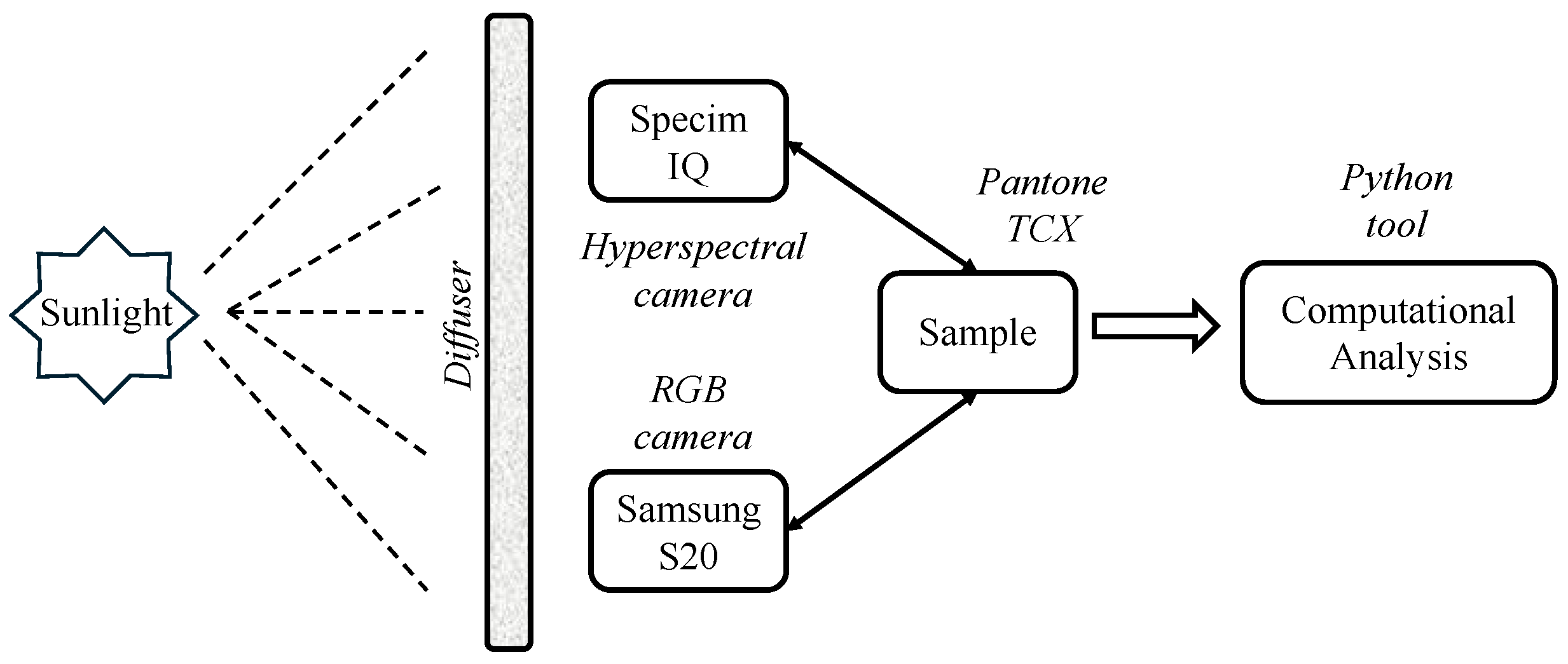
Figure 2.
Flowchart of the Python tool developed for reading, processing, segmenting, and transforming hyperspectral and RGB images into the CIE-L* a* b* color space. The images illustrate the step-by-step transformation applied to data as part of the computational algorithm.
Figure 2.
Flowchart of the Python tool developed for reading, processing, segmenting, and transforming hyperspectral and RGB images into the CIE-L* a* b* color space. The images illustrate the step-by-step transformation applied to data as part of the computational algorithm.
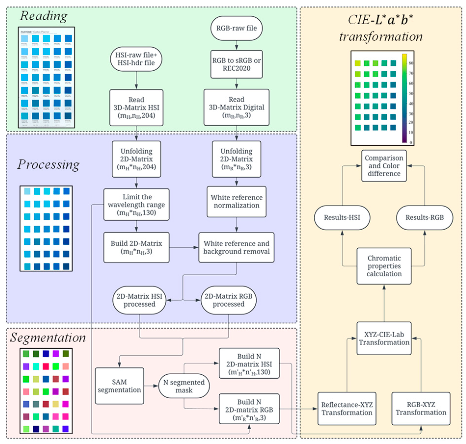
Figure 3.
Reflectance spectrum of 16 representative Pantone ® fabrics samples (TCX) in the visible range (400-750 nm) separated by light (solid line) and dark (dash line) colors in the chromatic regions of (a) red-yellow, (b) yellow-green, (c) green-blue and (d) blue-purple. The detection bands R (red), G (green) and B (blue) are included (vertical dash lines) as reference to correlate the spectral fingerprint with the corresponding RGB data.
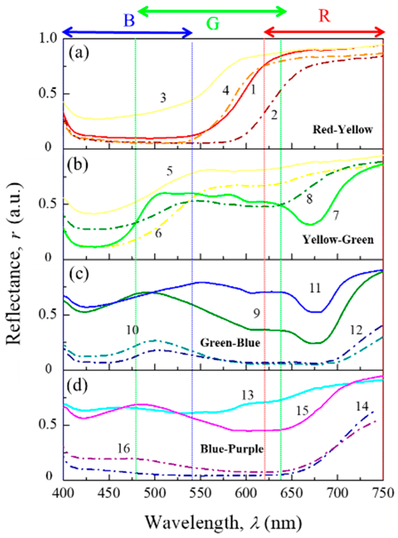
Figure 4.
Scatter plots of the chromatic properties (a) lightness , (b) , (c) , (d) chroma, (e) hue and (f) saturation, obtained from hyperspectral and RGB images in the representations sRGB (black) and REC2020 (red). The dash blue line is included in each case as a reference to observing the region of better agreement between HSI and RGB data. The icons in saturation plot have been separated by quadrant: squares (Q1), circles (Q2), triangles (Q3) and stars (Q4).
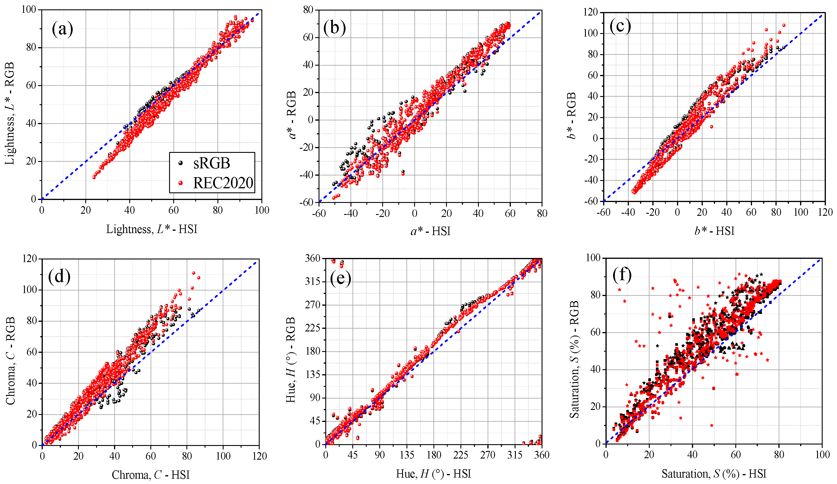
Figure 5.
(a) Scatter plot of the -stimulus obtained from HSI images and absolute color difference (∆E) between HSI and RGB data, for the 700 Pantone ® fabric samples (TCX) in sRGB (black) and REC2020 (red) representations. The icons have been separated by quadrants: squares (Q1), circles (Q2), triangles (Q3) and stars (Q4). (b) CIE- chromaticity and (c) CIE- diagrams displaying the coordinates of six samples with different -stimulus values. Circle the samples outside the volume.
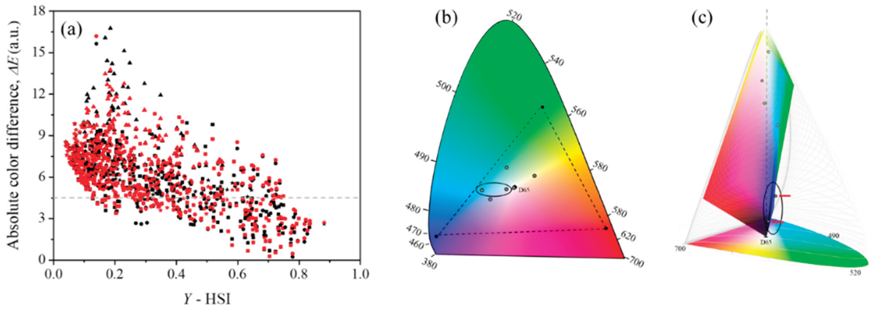

Table 1.
Statistical analysis of the chromatic properties obtained using hyperspectral images separated by quadrants (Q) in terms of the (lightness) (chroma), (hue) and (Saturation) for the 700 Pantone ® fabric samples (TCX).
Table 1.
Statistical analysis of the chromatic properties obtained using hyperspectral images separated by quadrants (Q) in terms of the (lightness) (chroma), (hue) and (Saturation) for the 700 Pantone ® fabric samples (TCX).
| Quadrant (N) |
* | ||||||
|---|---|---|---|---|---|---|---|
| L* | a* | b* | C | H | S | ||
|
Q1 (271) |
59.11 | 24.58 | 18.56 | 34.00 | 39.20 | 45.78 | |
| 55.72 | 16.62 | 11.85 | 27.61 | 33.93 | 46.59 | ||
| 27.02 | 0.02 | 0.08 | 1.93 | 0.22 | 3.63 | ||
| 93.15 | 59.51 | 86.45 | 86.55 | 89.85 | 80.60 | ||
| 1.35 | 2.81 | 2.02 | 2.38 | 1.92 | 2.37 | ||
|
Q2 (168) |
65.41 | -15.44 | 21.35 | 29.54 | 129.06 | 38.86 | |
| 65.88 | -13.18 | 15.39 | 26.67 | 129.85 | 38.48 | ||
| 31.07 | -50.69 | 0.31 | 3.50 | 90.14 | 5.20 | ||
| 93.73 | -0.02 | 81.20 | 81.35 | 179.39 | 68.36 | ||
| 1.96 | 1.10 | 1.45 | 1.35 | 2.06 | 2.85 | ||
|
Q3 (126) |
56.70 | -19.39 | -19.73 | 31.27 | 226.67 | 48.52 | |
| 55.03 | -18.42 | -21.61 | 32.27 | 227.20 | 50.22 | ||
| 30.60 | -46.16 | -36.13 | 3.60 | 180.04 | 11.69 | ||
| 83.73 | -0.27 | -0.03 | 46.16 | 269.52 | 67.50 | ||
| 2.72 | 0.78 | 2.81 | 1.82 | 2.23 | 2.39 | ||
|
Q4 (135) |
49.79 | 22.18 | -12.28 | 28.08 | 325.64 | 47.53 | |
| 45.34 | 19.11 | -12.38 | 29.31 | 333.50 | 52.19 | ||
| 23.79 | 0.79 | -34.89 | 2.44 | 271.74 | 6.23 | ||
| 95.72 | 56.16 | -0.10 | 56.20 | 359.23 | 76.09 | ||
| 1.96 | 2.51 | 1.86 | 2.75 | 2.20 | 2.55 | ||
N: number of samples, average value, median, minimum, maximum, average difference between HSI and Pantone® CIE-L*a*b* properties.
Table 2.
Accuracy of RGB images in reproducing the chromatic properties L* (lightness), a*, b*, C (chroma), H (hue), and S (saturation), evaluated using the ratio of performance to deviation (RPD). The information has been separated by quadrant (Q) and intervals for sRGB and REC2020 representations.
| * | * | * | |||||
|---|---|---|---|---|---|---|---|
| RPD | |||||||
| Q1 | sRGB | 4.67 | 3.07 | 1.65 | 2.15 | 1.17 | 2.42 |
| REC 2020 | 4.41 | 3.32 | 1.64 | 2.13 | 0.85 | 2.50 | |
| Q2 | sRGB | 3.22 | 1.94 | 4.36 | 3.18 | 2.45 | 2.31 |
| REC 2020 | 3.23 | 1.83 | 3.57 | 2.80 | 2.31 | 2.17 | |
| Q3 | sRGB | 1.75 | 1.01 | 0.96 | 0.83 | 1.20 | 0.93 |
| REC 2020 | 1.60 | 1.46 | 0.87 | 0.84 | 1.41 | 0.87 | |
| Q4 | sRGB | 2.53 | 1.34 | 1.64 | 1.17 | 0.37 | 1.30 |
| REC 2020 | 2.41 | 1.44 | 1.75 | 1.20 | 0.74 | 1.28 | |
| 50 | sRGB | 0.87 | 2.56 | 1.89 | 1.66 | 2.07 | 1.43 |
| REC 2020 | 0.83 | 2.77 | 2.08 | 1.74 | 2.29 | 1.44 | |
| 50 | sRGB | 3.48 | 3.38 | 2.85 | 2.08 | 3.61 | 2.44 |
| REC 2020 | 3.28 | 3.91 | 2.57 | 1.97 | 3.14 | 2.39 | |
Table 3.
Average of the absolute () and relative () color differences obtained by comparing HSI and RGB data in the sRGB and REC2020 representations. The information has been separated by quadrant (Q) and L* intervals for the 700 Pantone ® fabric samples (TCX). The standard deviation () is included to show the precision of the results.
| Samples | sRGB | REC 2020 | ||||||
|---|---|---|---|---|---|---|---|---|
| Q1 | 5.68 | 2.03 | 1.68 | 1.35 | 5.57 | 2.03 | 1.89 | 1.38 |
| Q2 | 5.57 | 2.51 | 2.74 | 2.94 | 5.71 | 2.42 | 2.94 | 2.90 |
| Q3 | 9.69 | 2.33 | 3.05 | 2.60 | 10.52 | 2.28 | 3.82 | 2.89 |
| Q4 | 6.80 | 1.45 | 4.17 | 3.74 | 6.74 | 1.66 | 4.67 | 3.78 |
| 50 | 7.54 | 1.73 | 4.19 | 3.31 | 7.43 | 1.59 | 4.50 | 3.40 |
| 50 | 5.72 | 2.67 | 1.71 | 1.78 | 5.68 | 2.51 | 1.97 | 1.94 |
| 75 | 3.91 | 1.77 | 1.04 | 0.87 | 4.03 | 1.86 | 1.22 | 0.99 |
Disclaimer/Publisher’s Note: The statements, opinions and data contained in all publications are solely those of the individual author(s) and contributor(s) and not of MDPI and/or the editor(s). MDPI and/or the editor(s) disclaim responsibility for any injury to people or property resulting from any ideas, methods, instructions or products referred to in the content. |
© 2025 by the authors. Licensee MDPI, Basel, Switzerland. This article is an open access article distributed under the terms and conditions of the Creative Commons Attribution (CC BY) license (http://creativecommons.org/licenses/by/4.0/).
Copyright: This open access article is published under a Creative Commons CC BY 4.0 license, which permit the free download, distribution, and reuse, provided that the author and preprint are cited in any reuse.


