
Submitted:
14 July 2025
Posted:
16 July 2025
You are already at the latest version
Abstract
Ash deposition on economizer heating surfaces degrades convective heat transfer efficiency and compromises boiler operational stability in coal-fired power plants. Conventional time-scheduled soot blowing strategies partially mitigate this issue but often cause excessive steam/energy consumption, conflicting with enterprise cost-saving and efficiency-enhancement goals. This study introduces an integrated framework combining real-time ash monitoring, dynamic process modeling, and predictive optimization to address these challenges. A modified soot blowing protocol was developed using combustion process parameters to quantify heating surface cleanliness via a cleanliness factor (CF) dataset. A comprehensive heat loss model was constructed by analyzing the full-cycle interaction between ash accumulation, blowing operations, and post-blowing refouling, incorporating steam consumption during blowing phases. An optimized subtraction-based mean value algorithm was applied to minimize cumulative heat loss by determining optimal blowing initiation/cessation thresholds. Furthermore, a bidirectional gated recurrent unit network with quantile regression (BiGRU-QR) was implemented for probabilistic blowing time prediction, capturing data distribution characteristics and prediction uncertainties. Validation on a 300 MW supercritical boiler in Guizhou demonstrated a 3.96% energy efficiency improvement, providing a practical solution for sustainable coal-fired power generation operations.
Keywords:
ash fouling
; economizer
; cleanliness factor
; subtraction-average-based optimizer
; quantile regression
; bi-directional gated recurrent units
1. Introduction
Achieving a green, low-carbon energy system [1,2] while ensuring energy security and sustainable development [3,4] is a global imperative. Within the critical transition of energy structures [5,6], coal-fired power remains indispensable, as evidenced by IEA data: coal dominates Asia-Pacific generation (57%), fossil fuels and nuclear power lead in the Americas (64%), and while natural gas prevails in Europe/Middle East (72%), coal still contributes 21%. In Africa, gas (42%) and coal/nuclear (34%) are primary sources [7]. Given that existing renewable energy infrastructure cannot yet fully supplant thermal power, enhancing the thermal efficiency of coal-fired units by minimizing heat losses is paramount. A major factor in the degradation of efficiency is the fouling of the ash on the surfaces of the boiler heat exchanger, making regular soot removal operations essential. Consequently, determining the optimal timing ("When?") and duration ("How long?") for soot-blowing is a persistent challenge in power plant operation and optimization.
Research into boiler efficiency optimization via soot-blowing includes various approaches. Wen et al. [8] formulated soot-blowing as an equipment health management problem using the Hamilton-Jacobi-Bellman equation and Markov processes. While enabling sensitivity analysis, its computational complexity hinders practical engineering application. Shi et al. [9] employed dynamic mass and energy balance for online thermal efficiency calculation and soft sensing to optimize soot-blowing frequency and duration without special instruments. However, this method assumes perfect cleaning after each cycle and lacks per-cycle effectiveness evaluation, limiting its robustness. Leveraging big data and deep learning, Pena et al. [10] developed probabilistic soot-blowing impact prediction models using ANNs and ANFIS, validated on a 350 MW plant. Xu et al. [11] combined the principles of heat balance, genetic algorithms (GA), and back propagation neural networks (BPNN) for dynamic monitoring and optimization of lag in a 650MW boiler, improving the net heat gain. Yet, traditional BPNNs struggle to capture dynamic heat loss trends accurately, affecting prediction fidelity. Kumari et al. [12] used an extended Kalman filter for Cleanliness Factor (CF) estimation and GA-GPR for prediction on a 210MW plant. However, dataset screening risks overlooking low-frequency variable influences, potentially biasing results.
Crucially, traditional single-point predictions do not quantify the uncertainty of the prediction, preventing operators from adjusting the proactive soot-blowing strategy.
Therefore, this case study focuses on the economizer of a 300MW coal-fired boiler in Guizhou province. We construct an ash deposition monitoring model based on key combustion parameters. The heat loss area under the economizer surface CF curve per cycle serves as the optimization objective function. An improved Subtraction-Average-Based Optimizer (SABO) is employed to evaluate and optimize the soot-blowing strategy for each cycle, identifying the soot-blowing node and duration minimizing heat loss. The target fouling segment for prediction is identified by applying the optimized node and threshold to operational data. Finally, a Quantile Regression-based interval prediction algorithm forecasts the target soot-blowing period within the time series. This integrated approach, combining thermodynamics and deep learning for holistic modeling, optimization, and prediction, aims to bridge mathematics and AI, enhancing practical soot-blowing optimization without excessive computational overhead, ultimately boosting economizer heat transfer efficiency.
The main contribution of this paper can be summarized in the following three points:
(1) In this paper, a dynamic multi-objective optimization model of heat loss for the whole process of economizer is established with the soot-blowing node and soot-blowing duration as the optimization objectives. It is more accurate and intuitive than previous models.
(2) Improvement of optimization algorithms for features of real problems so that the improved algorithms have higher convergence speed and convergence accuracy when facing specific issues.
(3) The interval prediction method based on quantile regression effectively reflects the overall distribution of the data and characterizes the uncertainty of the predicted point distribution, thereby improving prediction accuracy.
The integrated modeling-optimization-prediction approach provided in this paper is also a better guide for practical engineering. It optimizes and quantifies the soot-blowing nodes and durations for each cycle. It also gives the boiler operator more time to prepare for soot-blowing operations and develop a more reasonable soot-blowing strategy.
2. Problem Description
2.1. Introduction to the Structure of the Boiler and Economizer
This study focuses on a 300MW coal-fired power station boiler located in Guizhou province of China. The boiler operates using a tangential combustion mode at four corners, as illustrated in the accompanying figure. The model of the boiler is HG-1210/25.73-HM6, characterized by a steam drum-type configuration. It is a once-through boiler that features primary intermediate reheat and operates under supercritical pressure with variable conditions. The boiler employs an atmospheric expansion start-up system that does not utilize a recirculation pump. It is designed with a single furnace, balanced ventilation, solid slag discharge, an all-steel frame, a fully suspended structure, a type layout, and tight closure. Furthermore, the boiler incorporates a medium-speed mill positive pressure direct blowing pulverizing system, with each furnace equipped with five coal pulverizers. Under the BMCR working conditions, four coal pulverizers are operational while one mill remains on standby. The fineness of the pulverized coal is R90 = 18/20% (design/check coal type). The schematic diagram of the boiler heat transfer flow chart is shown in Figure 1
The type of economizer is cast-iron economizer, and its internal structure is shown in Figure 2. It is installed in the vertical flue at the end of the boiler and is used to recover the waste heat in the exhaust gas from the equipment; the boiler feed water is heated into the saturated water under the pressure of the steam natural circulation system of the heated surface since it absorbs high-temperature flue gas heat, reduces the temperature of the flue gas, saves energy, improves the efficiency, so it is called the coal economizer. It has many functions, for instance:
- Absorbing the heat of low-temperature flue gas, lowering the exhaust temperature, reducing sensible heat loss of the flue gas, and saving fuel.
- Increase the temperature of boiler feed water so that the feed water into the steam drum after the wall temperature difference is reduced, the thermal stress is reduced accordingly to extend the service life of the steam drum, etc.
Convection heat transfer is mainly embodied in the flue gas heating water, so the flue gas temperature is reduced simultaneously to enhance the feedwater temperature.
2.2. Grey Pollution Monitoring Model Construction
The heat transfer method of the coal economizer is mainly convection heat transfer, as shown in Figure 3, taking a single cast iron ribbed pipe as an example, the surface of the ribbed piece accumulates ash and scaling, which will reduce the convective heat transfer efficiency of the economizer.
In this study, the boiler’s cleanliness factor () dataset is classified and screened for soot-blowing node optimization, ash scaling monitoring, scaling prediction, improvement of heat transfer efficiency, and development of a more rational soot-blowing strategy. Generally, due to the complex working conditions of the heat transfer surfaces in a boiler, the ash accumulation state on the heat transfer surfaces cannot be measured directly. The boiler’s ash fouling state, combined with indirect parameters, can reflect the fouling accumulation state of the heat transfer surfaces. In this paper, the represents the ash fouling state:
where and are the heat transfer coefficients of the heat transfer surface and the theoretical heat transfer coefficient, respectively. The values of lie in the interval [0, 1], with one corresponding to the clean status of the heat transfer surface.
At this point, it is important to highlight the construction process of the soot monitoring model. The theoretical heat transfer coefficient is the heat transfer efficiency of the heating surface in the original light pipe state without soot deposition. It is usually the sum of the theoretical radiation heat transfer coefficient and the theoretical convective heat transfer coefficient, ignoring the thermal resistance between the working medium and the pipe wall as well as the internal thermal resistance of the metal.
where is the theoretical radiation heat transfer coefficient and is the theoretical convection heat transfer coefficient. The following mechanism equation usually obtains the heat transfer coefficient of the heated surface:
Where, and are the blackness of the tube wall and flue gas, respectively; T and are the temperatures of the flue gas and the tube wall, respectively, ℃; and are the transverse and longitudinal structural parameters of the heated surface of the economizer, respectively; is the thermal conductivity of the flue gas; d is the diameter of the tube in m; is the Reynolds number; is the flow rate of the flue gas in ; is the kinetic viscosity of the flue gas; and is the Plumtree constant.
The flue gas flow rate can be found from the Equation (6)
Where A is the heat transfer surface of the convection heat transfer surface, unit ; is the flue gas flow rate through the convective heating surface at standard conditions in , which can be obtained by measuring the actual flue gas flow rate via the Crabtree property.
Where is the actual measured flue gas flow rate in ; is the measured temperature of the flue gas in the section, ℃; is the pressure of the flue gas, ; is the standard atmospheric pressure, .
The actual heat transfer coefficients are obtained through a dynamic energy balance.
Where is the heat released by the flue gas flowing through the heated surface, ; is the average temperature difference between the flue gas side and the mass side of the heat transfer surface, .
Considering the energy balance between the flue gas side and the work mass side, the heat released by the flue gas on the flue gas side, , is equal to the heat absorbed by the work mass on the work mass side, (), there is:
Heat absorbed on the work side
Where D is the work mass flow rate through the heated surface, ; and are the enthalpy of the work mass flowing through the outlet and inlet of the heated surface, , respectively. and are calculated using the [12] formula.Where the saturated steam parameters , temperature , pressure P for .
The calculated CF image with the normalized load profile is shown in Figure 4.
3. Full Process Modeling of Economizer Energy Efficiency
3.1. Raw Data Plotting
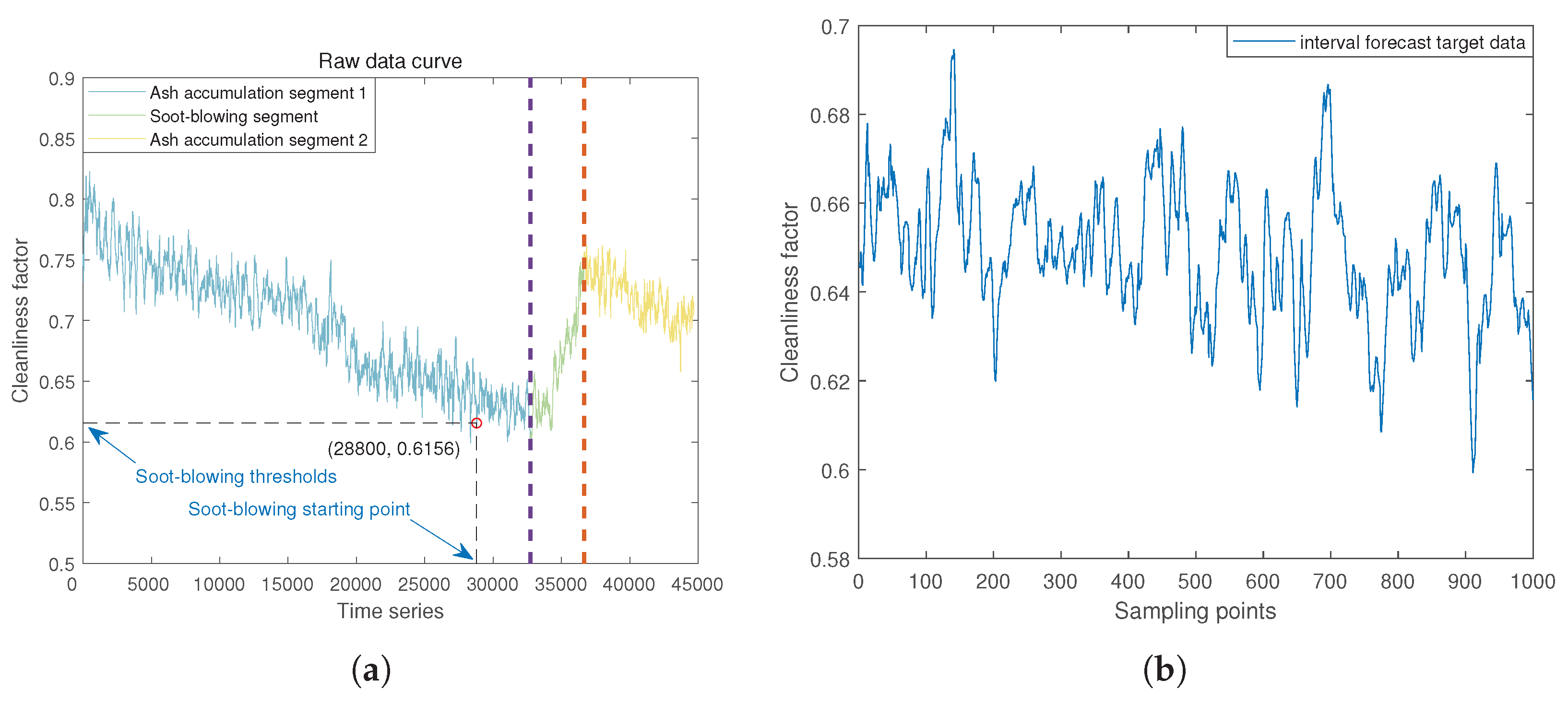
In the axes shown in Figure 5, the indigo blue curve is the soot accumulation segment 1, the green curve is the soot-blowing segment, the yellow curve is the soot accumulation segment 2, the two purple and red dotted lines indicate the soot-blowing start point and the soot-blowing endpoint, respectively, and the vertical coordinate indicates the trend of the change of cleanliness factor, and the horizontal coordinate indicates the time, with a sampling period of 5 seconds.
3.2. Data Pre-Processing
Since the curve of the original data of the coal economizer cleanliness factor (shown in Figure 5) is non-linear and non-stable, the direct calculation of the area by a definite integral will produce a large error, so we use the polynomial fitting method to deal with the original data. The expression for the polynomial fit is:
After obtaining the fitted curve, reduce the calculation error by calculating the boundary and the fitted curve enclosing the area, which is convenient for calculating the area. The polynomial fitting results and expressions for the three processes for the trend change in the cleanliness coefficient of the economizer are shown in Figure 6. The polynomials corresponding to ash accumulation segment 1, soot-blowing segment, and ash accumulation segment 2 are Equation (12), (13) and (14), respectively.
3.3. Optimization Problem Description
Figure 7 a schematic diagram of the reduction of heat transfer coefficient from the heated surface of the economizer. The area of the curved trapezium enclosed by the fitted curve with , , is .
The area of the curved trapezium enclosed by the fitted curve with , , is . is used as the soot-blowing stage and includes a portion of the steam loss [13]. Since the soot-blowing method is used in the 300MW unit of the Guizhou power plant, the research object is steam soot-blowing, and steam loss is inevitably caused during soot-blowing operations. In this study, steam loss is used as part of the fitness function of the optimization problem to optimize the entire soot-accumulation-soot-blowing-soot-accumulation cycle globally.
represents the soot-blowing steam flow rate in , represents the soot-blowing time in s, and represents the enthalpy of the soot-blowing steam source in , while represents the enthalpy of the condenser inlet steam in .
The area of the curved trapezium enclosed by the fitted curve with , , is . The total area of heat loss for these three operating processes of the economizer is:
is the sum of the heat losses from the three processes on the heating surface of the heat accumulator and is also the objective function of the optimization problem. When ,, the heat loss area at the heated surface of the economizer before the optimization is 12836.7124. At this time, the percentage heat loss from the heated surface of the economizer is:
The percentage reduction of heat transfer coefficient of the original economizer dataset is 28.7239%.
4. Improved Subtraction-Average-Based Optimizer and Optimization Results
4.1. Subtraction-Average-Based Optimizer
The idea of SABO’s algorithm [14] is to update the positions of the population members in the search space using the subtracted averages of multiple intelligences, such as the mean, the difference in the positions of the search agents, and the sign of the difference between the two values of the objective function, using the arithmetic average position of all the search agents. SABO is based on the special operation“” called subtraction from search agent A to search agent B, expressed as:
The displacement of any search agent in the search space is computed by the arithmetic mean of the subtractions of each search agent :
Determine whether to accept a new agent:
The illustration of the use of "v-subtraction" for exploration and mining is shown in Figure 8:
4.2. Golden Ratio Strategy
Traditional optimization algorithms are inefficient in interval partitioning as they require more function evaluations to narrow the search interval. For some gradient-based algorithms, it is easy to fall into topical optimal solutions, and the golden ratio strategy is a global search method that helps avoid premature convergence to topical minima or maxima.
(1) Initialization intervals: Set an initial search interval [a, b], where a and b are the upper and lower bounds of the solution space.
(2) Determine the subinterval: the interval [a, b] is divided into two subintervals according to the golden ratio. Let c and d be two points in the interval such that:
, it is a mathematically specific ratio.
(3) Evaluation function value: Compute and . is the objective function, and we want to find the minimal or maximal value of in this interval.
(4) Update interval: Compare the values of and ; if the new search interval becomes [a, d]; on the contrary, if the new search interval becomes [c, b]. After each iteration, the length of the interval is reduced according to the golden ratio.
(5) Repeat steps (2) to (4) until the length of the search interval is less than a predefined threshold or an upper limit on the number of iterations is reached.
4.3. Piecewise Chaos Mapping
In many traditional optimization algorithms, the initialization of the population is not random enough, leading to premature convergence of the algorithm to the topical optimal solution, which fails to achieve the desired effect. To address this problem, piecewise chaos mapping has been added to the algorithm for further improvement. Piecewise chaos mapping has good statistical performance and is a segmented mapping function. The piecewise chaos mapping formula is:
P takes values in [0, 0.5], a segmented control factor used to divide the 4-part function of this segmented function. Generally, . The range of chaotic orbital state values is (0, 1). The effect of population initialization with adding Piecewise chaos mapping is shown in Figure 9.
4.4. Roulette Wheel Selection
Since the objective problem with nonlinear constraints solved in this paper is minimization, the probability of the optimal solution appearing at the boundary is much higher. The insensitivity of traditional optimization algorithms to boundary values makes the optimal solution easy to ignore. Most optimization algorithms have only one process, which makes it easy for non-optimal solutions to be selected.
The roulette strategy is one of the commonly used strategies in genetic algorithms.
(1) Proportions the probability of an individual being selected with the size of its fitness value (as shown in Equation (24)).
is a certain individual.
(2) Cumulative probability represents the probability of everyone using line segments of different lengths, which are combined to form a straight line with a length of 1 (the sum of the probability of everyone), such that the longest line segment of a certain segment in the line represents the higher probability of the individual being selected. Its mechanism is:
- Arbitrarily selecting a sequence of permutations of all individuals (this sequence can be arbitrary because it is the length between certain line segments as representing the probability of selection of a particular individual)
- The cumulative probability of any individual (as shown in Equation (25)) is the cumulative sum of the previous data corresponding to that individual.
(3) Generate a random number between the intervals [0, 1], and it is judged in which interval the number falls, and if it falls in a certain interval, that interval is selected. Obviously, for an individual with a larger fitness value, the length of the corresponding line segment will be long. Hence, the probability of a randomly generated number falling in this interval is large, and the probability of that individual being selected is also large. Figure 10 shows a simple example of four independent trials using the roulette wheel selection algorithm
In this paper, we also extend the single process of the algorithm to multi-process by converting the fitness of the individuals in each process into a probability, eliminating the individual with the smallest probability, and looping the others into the next process. After many experiments, the optimal solution can be locked in about three cycles.
4.5. Solving Targeted Problems with GRSABO
In the subSection 3.3 of this paper, the objective function of the GRSABO algorithm is obtained. Now, we set (ashes-blowing starting point) and (soot-blowing endpoint) as unknown variables, and let and move freely on the subject to the constraints. The main task of the optimization part of this paper is to minimize the value of by varying the values of and . As shown in Figure 11.
According to the operating regulations of thermal power plants, the interval between two soot-blowing operations cannot be less than 8 hours(), and the duration of each soot-blowing is in the range of 4500 to 5400 seconds(), which are the two non-linear constraints of the optimization problem.
4.6. Optimization Results and Validation
In this paper, six intelligent optimization algorithms are used, such as the whale optimization algorithm (WOA), the gray wolf optimization algorithm (GWO), the subtraction-average-based Optimizer (SABO), the particle swarm optimization algorithm (PSO), the seagull optimization algorithm (SOA), and the sparrow optimization algorithm (SSA) in the comparison of the improved subtraction-average-based Optimizer. 20 independent trials of each optimization algorithm on the objective function, the starting point of ashes blowing , the endpoint of soot blowing , and the heat loss area of the heated surface of the economizer obtained from each experiment were recorded. The results obtained by the seven optimization algorithms are plotted in box plots of , and respectively, and the results obtained are analyzed. Firstly, through all the experiments, we get the minimum value of as 11057.3562, which corresponds to value of 28800 and value of 33300.
Figure 12(a) shows the soot-blowing starting points obtained by seven optimization algorithms. represents the value of when is at its smallest, and by the box plot, the results of the 20 experiments of GRSABO converge more efficiently around 28800 and have fewer outliers.
Figure 12(b) shows the experimental results at the endpoint of soot-blowing obtained by seven different optimization algorithms. represents the value of when is at its smallest point, and through the box plots, the results of the 20 experiments of GRSABO converge more efficiently and with fewer outliers around 33300.
Figure 12(c) shows the experimental results of the heat loss area of the heated surface of the economizer obtained by seven different optimization algorithms, and through the box plots, the results of the 20 experiments of GRSABO converge more efficiently around y = 11057.3562 and with fewer outliers. The optimized thermal efficiency of the heated surface of the economizer is shown in Equation (26)
In summary, GRSABO shows a clear advantage over other optimization algorithms in its convergence accuracy. Throughout the optimization module, we obtain the ideal soot-blowing starting point , soot-blowing endpoint , and the heat loss area of the heating surface of the economizer . This paper will use this soot-blowing threshold point in the prediction module to perform interval prediction. Table 1 shows the optimal solutions selected by different optimization algorithms and the frequency of selection of optimal solutions in 20 independent trials. After algorithmic optimization, the thermal efficiency of the economizer is increased by approx:

Table 1.
Comparison of optimal solutions of 7 optimization algorithms and frequency of occurrence of optimal solutions.
Table 1.
Comparison of optimal solutions of 7 optimization algorithms and frequency of occurrence of optimal solutions.
| Optimization algorithms | |||
|---|---|---|---|
| WOA | 29000 | 33500 | 11324.74 |
| GWO | 28890 | 33432 | 11187.51 |
| SABO | 28800 | 33300 | 11057.36 |
| PSO | 28800 | 33308 | 11058.48 |
| SOA | 28800 | 33400 | 11071.07 |
| SSA | 28800 | 33378 | 11068.12 |
| GRSABO | 28800 | 33300 | 11057.36 |
5. Optimization Results Applied to Interval Prediction
5.1. Integration and Application of Optimization Results
According to subSection 4.6, we obtain the optimized soot-blowing start point and the corresponding soot-blowing threshold, bring the soot-blowing threshold and the soot-blowing start point into the original cleanliness factor dataset, and intercept the 1000 sets of data before the soot-blowing threshold. We have the soot accumulation segment for which we will perform interval prediction.
Figure 13.
(a) Optimization results graphic. (b) Interval forecast target data.
5.2. Wavelet Thresholding Method for Denoising
The wavelet threshold noise removal method [15,16] is a time-frequency localization analysis method. After the wavelet transforms the signal, the signal is decomposed into several sub-bands of time domain components. The noise signals with small wavelet coefficients can be filtered by selecting appropriate threshold values. Too large a threshold value will cause the loss of effective information, while too small a threshold value will cause the residual noise signal, affecting the prediction results’ accuracy.
The steps of wavelet threshold denoising are as follows:
(1) For the original signal characteristics and application background, select the appropriate wavelet basis find the number of layers, and use wavelet decomposition to process the original signal containing noise to obtain the wavelet coefficients [17].
(2) After selecting a suitable threshold, the threshold function processes the layer coefficients [18]. Considering that the hard threshold function will cause the reconstructed signal to oscillate and the soft threshold signal will easily lead to signal distortion when dealing with nonlinear signals, the unbiased risk estimation threshold is selected as the threshold function in this paper.
The unbiased risk estimation threshold function is calculated as follows:
- The absolute values of all elements in the original signal are first extracted, and then the sequence of absolute values is ordered from smallest to largest. The expression is:
- Set be the square root of the jth element of
- Then the risk function with this threshold is shown in Equation (30)
- vvThe corresponding risk curve can be obtained from the risk function, and then the value of j corresponding to the smallest risk is recorded as , and the unbiased risk estimation threshold can be obtained from .(3) The signal after noise removal is obtained by processing the wavelet coefficients with the unbiased risk estimation threshold.
Here, we evaluate the denoising effect using three metrics: signal-to-noise ratio (SNR), root-mean-square error (RMSE), and running time. The signal-to-noise ratio (SNR) and root-mean-square error (RMSE) are shown in Equation (32) and Equation (33):
where is the signal power, is the noise power, n is the number of observations, is the true value of the ith observation. is the predicted value of the observation.
5.3. Ensemble Empirical Mode Decomposition
The traditional empirical modal decomposition (EMD) [19] has significant advantages when dealing with nonlinear and non-smooth time series; it is based on the distribution of the extreme points of the signal itself, so there is no need to choose a basis function, and in addition, it is data-driven and adaptive. It is not constrained by Heisenberg’s principle of inappropriateness of measurement [20,21]. However, EMD is highly susceptible to modal aliasing. Modal aliasing leads to false time-frequency distributions and renders the IMFs physically meaningless. Ensemble empirical modal decomposition(EEMD) [22] is an improved version of EMD, which reduces the problem of modal aliasing in EMD by adding Gaussian white noise to the original signal and then performing EMD decomposition of multiple noisy versions of the signal finally averaging the results. Here are the basic steps of EEMD:
(1) Add Gaussian white noise: add a set of randomly generated Gaussian white noise to the original signal to create a set of noise-added signals , i is the number of times the noise is added [23,24].
(2) EMD decomposition: an EMD decomposition is performed for each noisy signal to obtain a series of intrinsic mode functions (IMFs). [25]
(3) Average treatment: the IMFs of the same sequences obtained from each noisy signal are averaged to obtain the final stable set of IMFs.
M is the number of IMF components.
Table 2.
Comparison of four threshold function evaluation indicators.
| Evaluation indicators | Rigrsure | Minimax | Sqtwolog | Heursure |
|---|---|---|---|---|
| SNR | 60.7562 | 53.5176 | 49.7381 | 51.3049 |
| RMSE | 0.000595 | 0.001369 | 0.002116 | 0.001767 |
| Runtime(second) | 0.3429 | 0.3517 | 0.3712 | 0.3498 |
5.4. T-Test
After using the EEMD decomposition, we need to classify and integrate the obtained IMF components to obtain three key features for interval prediction: high-frequency components, low-frequency components, and trend terms, and the method for integrating these features t-test [25,26] is described below. The obtained IMF components were preprocessed by noting IMF1 as indicator 1, IMF1+IMF2 as indicator 2, and so on, with the sum of the first i IMF components adding up to indicator i. A T-test was performed to determine whether this mean differed significantly from 0. The specific steps of the t-test are as follows:
(1) Set the assumptions: Null hypothesis(): The mean of the sample is equal to 0. Alternative hypothesis(): The sample’s mean is not equal to 0.
(2) Selecting the significance level: usually, = 0.05 is chosen as the significance level. We will reject the null hypothesis if there is a 5% probability that the observed data is inconsistent with the hypothesized overall mean.[27]
(3) Calculating t-statistics: statistics calculation using Equation (36).
is the sample mean, is the hypothesized overall mean, s is the sample standard deviation and n is the sample size.
(4) Determining sample degrees of freedom (): .
(5) Finding the t critical value: find the t critical value corresponding to the degree of freedom () and significance level () in the t distribution table.
(6) Comparing t-statistics and t-critical values: if the absolute value of the calculated t-statistic is greater than the t critical value, the null hypothesis is rejected, and the sample mean is considered to be significantly different from 0.
(7) Conclusion: If the absolute value of the t statistic is greater than the t-critical value, then you can conclude that the sample mean is significantly different from 0, based on the direction of the alternative hypothesis.
If the absolute value of the t-statistic is less than or equal to the t-critical value, then you cannot reject the null hypothesis; there is not enough evidence that the sample mean is significantly different from 0.
5.5. Interval Forecasting
5.5.1. Quantile Regression
The main goal of traditional mean regression (OLS) [28] is to estimate the conditional mean of the dependent variable (response variable) about one or more independent variables (explanatory variables). In the simplest case, the OLS regression attempts to find a straight line (or hyperplane in multidimensional space) such that the sum of the squares of the distances (residuals) of all observations from this line is minimized. This means that the OLS regression estimates the model parameters by reducing the residual sum of squares (RSS). OLS regression is usually required to satisfy several assumptions, such as zero mean of the error term, homoskedasticity, no autocorrelation, etc. At the same time, it is susceptible to extreme values or outliers because the squares amplify the larger residuals. Therefore the OLS regression cannot portray the uncertainty of the predicted points [29].
Quantile regression (QR) aims to estimate the relationship between the dependent and independent variables at different quantile levels, not just the mean. For example, it can estimate the regression relationship for median regression (When the quantile ), upper quartile regression (), or other regression relationships at any quantile level. Quantile regression uses different loss functions to minimize a weighted sum of the absolute values of the residuals, with the weights depending on the direction of the residuals and the chosen quantile level. Quantile regression [30] is more robust to outliers because it uses the absolute value of the residuals rather than the square. It also allows for heterogeneity analysis, permitting analyses of how the effect of the dependent variable may vary across quartiles, providing more comprehensive information about the relationship between variables. At the same time, quantile regression does not require that the error term obey a particular distribution or that homoskedasticity be present [31].
Quantile regression is usually divided into 5 steps as follows:
(1) Data preparation: Determine the response variable Y and explanatory variable X. Split the dataset into a training set and a test set.
(2) Model setting: Set the form of the quantile regression model, which is usually a linear model: , where is the th quantile of Y for a given, X and is the corresponding regression coefficient.
(3) Definition of loss function: Quantile regression uses a special loss function that adjusts the weights according to the sign of the residuals. The loss function is defined as:
is the residual, and is the quantile (between 0 and 1) one wants to estimate.
(4) Parameter estimation: The parameter is estimated by minimizing the overall loss function.
Here, and are the response and explanatory variables for the ith observation, respectively.
(5) Model validation: Using test set data to assess a model’s predictive power, some measure of error between predicted and actual values can be calculated, such as mean absolute error (MAE) or quantile absolute deviation (QAD).
(6) Model interpretation: analyze the estimates of to understand the effect of the explanatory variables on the response variable at a particular quantile level.
5.5.2. Gated Recurrent Unit
Gated recurrent unit (GRU) [32] is a type of recurrent neural network, an improvement of recurrent neural network (RNN) and long short-term memory network (LSTM) [33], which can better capture dependencies on sequences with a long time-step distance, Reset Gate helps to capture short-term dependencies in sequences; Update Gate helps to capture long-term dependencies in sequences. When the reset gate is open, the gated recurrent unit contains the basic recurrent neural network; when the update gate is open, the gated recurrent neural unit can skip subsequences. Figure 14 shows the internal structure of GRU.
Firstly, we obtain two gating states from the last transmission state and the current node’s input . Where controls reset gating and controls update gating.
is the sigmoid function by which the data is normalized to a value between [0,1], which acts as a gating signal. ,, W is a machine learning process that replaces the weights with new ones after each iteration.
After getting the gating signal, use the reset gating to get the data after the "reset," where ⊙ is the Hadamard Product.
Splicing with the input and then normalizing the data to values between [-1,1] by the activation function yields the candidate value , contains the signal features in the current input and adds the new features recorded through learning.
The most critical step of GRU - "updating memory" - is the step in which both "forgetting" and "remembering" take place.
The closer the gating signal is to 1, the more data is "remembered," and the closer it is to 0, the more data is "forgotten."
5.5.3. Bidirectional Gating Unit
A bidirectional gating unit (BiGRU) is essentially a two-layer GRU network, where features are fed into the network training through forward propagation in the forward GRU layer while mining the forward correlation of the data. In the reverse GRU layer, the input sequences are trained by back-propagation to mine the inverse correlation of the data, and this network architecture allows for bidirectional extraction of the input features to enhance the completeness and global nature of the features. Figure 15 shows the internal structure of the BiGRU.
5.5.4. An Interval Prediction Method Incorporating EEMD-QRBiGRU
Since a single BiGRU model can only learn the deterministic mapping relationship between the input features and the prediction target and cannot reflect the information, such as its uncertainty error distribution in the prediction results, this paper combines the theory of quantile regression. It proposes a BiGRU prediction model based on quantile regression, which can realize the prediction of the trend of the coal economizer cleaning factor under different quantiles and thus achieve the function of interval prediction.
The parameters in the BiGRU model are the weights W and bias vectors b of each neuron. The quantile regression method is introduced into the neural network to establish the BiGRU model based on the quantile regression loss function. The conditional quantile of the output response variable Y at the quantile is:
where J is the number of units of the hidden state, f is the activation function of the output layer, is the output of the BiGRU hidden state, and and are the weight and bias of the output layer respectively.
Updating the network parameters according to the gradient descent algorithm (Adam) yields l BiGRU models with different weights and biases. After a series of forward propagation and backward learning, the predicted values of the response variables under each quantile at the moment can be obtained:
This enables the estimation of the probability density distribution of , as well as the calculation of confidence intervals for from discrete conditional quartiles.
where is the prediction interval at the significance level, and are the upper and lower limits of the prediction interval, respectively, and , the confidence level of the interval is .
In summary, the prediction process of the proposed EEMD-QRLSTM is shown in Figure 16, and its algorithm execution steps are as follows:
- Denoising the original data using the wavelet thresholding method
- Decompose the denoised data into EEMD data, and obtain 9 sets of IMF components after decomposition.
- Classify the IMF components using the t-test to obtain three features: high-frequency components, low-frequency components, and trend terms.
- Determine the structure of the network, the number of nodes, and the number of quantile points l, initialize the network, and construct the training set and test set;
- Input the training set into QRBiGRU, train and update the BiGRU model under each quantile point ;
- The explanatory variable from the test set is entered into the trained QRBiGRU to obtain the conditional quantile of the response variable at time t and output the results.
6. Interval Prediction Result Display
6.1. Wavelet Thresholding Method Denoising Module
In this paper, four different threshold functions are used to process the raw data (as shown in Figure 17), namely Rigrsure: unbiased risk estimation threshold, Heursure: heuristic threshold function, Minimax: substantial and tiny thresholds, and Sqtwolog: fixed thresholds Evaluation metrics of the results of the four threshold functions are shown in Table 3.
By comparing the evaluation indexes, we find that the unbiased risk estimation threshold has the highest signal-to-noise ratio with the smallest root-mean-square error, and it also has the shortest running time, so in this paper, we use the unbiased risk estimation threshold function to deal with the optimized time series.
6.2. Modal Decomposition of the Cleanliness Factor Time Series Using EEMD and Classification Using T-Test
The data after wavelet threshold denoising still have nonlinear and non-smooth characteristics. Hence, it needs to be further subjected to ensemble empirical modal decomposition (EEMD) to get the topical signals containing different time scales of the original signals: the intrinsic mode function components (IMFs), which are shown in Figure 18, and after decomposition, eight Intrinsic Mode Function components and a trend term are obtained.
After the ensemble empirical modal decomposition, a t-test is needed to classify these Intrinsic Mode Function components into three categories: high-frequency components, low-frequency components, and trend terms. Knowing that RES is the trend term, IMF1 is defined as indicator 1, IMF1 + IMF2 is defined as indicator 2, and so on, comparing the t-values of indicator 1 and indicator 2, indicator 2 and indicator 3, respectively. We find that the t-values at indicator 7 and indicator 8 are close to 0, which indicates that IMF1∽IMF7 are high-frequency components, and IMF8 are low-frequency components.
6.3. BiGRU Time Series Forecasting Based on Quantile Regression
After obtaining the three key features, the high-frequency component, the low-frequency component, and the trend term, interval prediction of the cumulative grey time series is performed using a two-way gated neural network based on quantile regression. Setting training set data: test set data = 8:2, the experimental results are obtained as shown in Figure 19.
In this paper, we use mean square error (MAPE), mean square error (MSE), interval coverage (PICP), and predicted interval average width (PINAW) as the evaluation metrics to evaluate the prediction effect of the test set and the training set.
The value of MAPE ranges from , with a MAPE of 0% indicating a perfect model and a MAPE greater than 100% indicating a poor quality model.
The range of values for MSE is , which is equal to 0 when the predicted value coincides exactly with the true value, and the model is perfect; the larger the error, the larger the MSE value.
is a Boolean variable, and represent the next and previous terms corresponding to the ith prediction interval, respectively, and represents the actual value. The closer the PICP is to 1, the higher the probability of falling into the prediction interval, which means the better the prediction is. However, when the prediction interval is wider, the coverage of the prediction interval will also increase, and the information that can be provided will be less, so this paper introduces the average bandwidth of the prediction interval (PINAW).
, R represents the extreme deviation from the true value. The smaller PINAW means a better prediction, and there is actually an inverse relationship between PICP and PINAW. The comparison of the evaluation metrics for the test set and the training set is shown in Table 4.
6.4. Comparison of the Results of 4 Prediction Models Based on Quantile Regression
Through the evaluation indexes of the above experiments, it can be seen that the bi-directional gated cyclic unit based on quantile regression is very effective in predicting the intervals of the accumulated grey segments, so can it perform better in comparison with other optimization algorithms for which this paper carries out the following kinds of comparisons. Including the comparison among QRBiGRU, QRBiLSTM, QRLSTM [34], QRGRU, and the original data.
From Figure 20, it can be seen that the prediction results of QRBiGRU have the highest degree of fit with the original data, and the following is a comparison of the evaluation indexes of the prediction results of these four methods. These evaluation indicators allow us to visualize the strengths and weaknesses of the prediction results more intuitively.
7. Conclusions
This study presents an integrated framework combining deep learning and quantile regression to optimize energy efficiency in coal-fired power plant economizers. A soot deposition monitoring model was developed using critical boiler combustion parameters to calculate the economizer’s cleanliness factor, enabling characterization of convective heat transfer efficiency. The derived heat loss function was optimized using an improved Generalized Subtraction-Average-Based Optimizer (GRSABO) algorithm to determine soot-blowing start/end points that minimize combined heat and steam loss . Subsequently, processed soot buildup segments underwent interval prediction through a Bidirectional GRU network integrated with quantile regression (QRBiGRU), effectively quantifying prediction uncertainty. Validation on a 300MW unit in Guizhou Province demonstrated QRBiGRU’s superior accuracy over benchmark models and achieved 4% improvement in heat transfer efficiency while robustly characterizing uncertainty distributions without complex computational overhead. The framework provides validated operational guidance for cost reduction and efficiency enhancement. Looking forward, developing adaptive digital twin models capable of accommodating diverse operating conditions and load fluctuations represents a critical pathway to address renewable energy intermittency, with this study providing a methodological foundation for such advancements in power plant digitalization.
Author Contributions
Conceptualization, Yuanhao Shi and Nan Wang; methodology, Fangshu Cui; software, Jie Wen; validation, Jianfang Jia; writing—original draft preparation, Nan Wang; validation, Nan Wang; writing—review and editing, Bohui Wang; funding acquisition, Fangshu Cui, Yuanhao Shi and Nan Wang.All authors have read and agreed to the published version of the manuscript.
Funding
This research was funded by the National Natural Science Foundation of China grant number 72071183, the Fundamental Research Program of Shanxi Province grant number 202303021222084 and Graduate School-level Science and Technology Project of the North university of China grant number 20242066
Conflicts of Interest
The authors declare no conflicts of interest.
Abbreviations
The following abbreviations are used in this manuscript:
| CF | Cleanliness Factor |
| BiGRU | Bi-directional Gated Recurrent Units |
| QR | Quantile Regression |
| SABO | Subtraction-Average-Based Optimizer |
| WOA | Whale Optimization Algorithm |
| GWO | Grey Wolf Optimization |
| PSO | Particle Swarm Optimization |
| SOA | Seagull Optimization Algorithm |
| SSA | Sparrow Search Algorithm |
| GA | Golden Sine Algorithm |
| EEMD | Ensemble Empirical Mode Decomposition |
| LSTM | Long Short-Term Memory |
| GRU | Gated Recurrent Units |
| MAPE | Mean Absolute Percentage Error |
| MSE | Mean Square Error |
| PICP | Prediction Interval Coverage Probability |
| PINAW | PI Normalized Average Width |
References
- Liu, P.; Peng, H. What drives the green and low-carbon energy transition in China?: An empirical analysis based on a novel framework. Energy 2022, 239, page. [Google Scholar] [CrossRef]
- Zhao, C. Is low-carbon energy technology a catalyst for driving green total factor productivity development? The case of China. J. Clean. Prod. 2023, Nov.20, 428. [Google Scholar] [CrossRef]
- Fang, D.; Shi, S.; Yu, Q. Evaluation of Sustainable Energy Security and an Empirical Analysis of China. Sustainability 2018, 10, 5. [Google Scholar] [CrossRef]
- Zakari, A.; Musibau, H.O. Sustainable economic development in OECD countries: Does energy security matter? Sustain. Dev. 2024, 1, 32. [Google Scholar] [CrossRef]
- Ning, Z.; Meimei, X.; Xiaoyu, W.; Hongcai, D.; Yunzhou, Z.; Lin, L.; Dong, Z. Comparison and Enlightenment of Energy Transition Between Domestic and International. Electr. Power 2021, 54, 02–113. [Google Scholar]
- Zhang, Y.N.; Liu, Y.N.; Ji, C.L. A research on sustainability evaluation and low-carbon economy in China. In: IOP Conf. Ser.: Earth Environ. Sci. 2019, 233, 052008. [Google Scholar] [CrossRef]
- Shuai, Y.; Zhao, B.; Jiang, D.F.; He, S.; Lyu, J.; Yue, G. Status and prospect of coal-fired high efficiency and clean power generation technology in China. Therm. Power Gener. 2022, 51, 1. [Google Scholar]
- Wen, J.; Shi, Y.; Pang, X.; Jia, J.; Zeng, J. Optimal soot blowing strategies in boiler systems with variable steam flow. In: Proc. 37th Chin. Control Conf. 2018, 2284–2289.
- Shi, Y.; Wang, J.; Liu, Z. On-line monitoring of ash fouling and soot-blowing optimization for convective heat exchanger in coal-fired power plant boiler. Appl. Therm. Eng. 2015, 78, 39–50. [Google Scholar] [CrossRef]
- Peña, B.; Teruel, E.; Díez, L.I. Soft-computing models for soot-blowing optimization in coal-fired utility boilers. Appl. Soft Comput. 2011, 11, 2–1657. [Google Scholar] [CrossRef]
- Xu, L.; Huang, Y.; Yue, J.; Dong, L.; Liu, L.; Zha, J.; Yu, M.; Chen, B.; Zhu, Z.; Liu, H. Improvement of slagging monitoring and soot-blowing of waterwall in a 650MWe coal-fired utility boiler. J. Energy Inst. 2021, 96, 106–120. [Google Scholar] [CrossRef]
- Bongartz, D.; Najman, J.; Mitsos, A. Deterministic global optimization of steam cycles using the IAPWS-IF97 model. Optim. Eng. 2020, 21, 1095–1131. [Google Scholar] [CrossRef]
- Zhu, Q. Developments in circulating fluidised bed combustion. IEA Clean Coal Cent. 2013, 300, 219. [Google Scholar]
- Trojovský, P.; Dehghani, M. A New Swarm-Inspired Metaheuristic Algorithm for Solving Optimization Problems. Biomimetics 2023, 8, 149. [Google Scholar] [CrossRef]
- Adebayo, T.S. Environmental consequences of fossil fuel in Spain amidst renewable energy consumption: a new insights from the wavelet-based Granger causality approach. Int. J. Sustain. Dev. World Ecol. 2022, 29, 7–579. [Google Scholar] [CrossRef]
- Chen, J.; Pan, J.; Li, Z.; Zi, Y.; Chen, X. Generator bearing fault diagnosis for wind turbine via empirical wavelet transform using measured vibration signals. Renew. Energy 2016, 89, 80–92. [Google Scholar] [CrossRef]
- Hao, L.; Naiman, D.Q. Quantile Regression; Sage: Thousand Oaks, CA, USA, 2007; Volume 149. [Google Scholar]
- Feng, X.; Li, Q.; Zhu, Y.; Hou, J.; Jin, L.; Wang, J. Artificial neural networks forecasting of PM2.5 pollution using air mass trajectory based geographic model and wavelet transformation. Atmos. Environ. 2015, 107, 118–128. [Google Scholar] [CrossRef]
- Perez-Ramirez, C.A.; Amezquita-Sanchez, J.P.; Valtierra-Rodriguez, M.; Adeli, H.; Dominguez-Gonzalez, A.; Romero-Troncoso, R.J. Recurrent neural network model with Bayesian training and mutual information for response prediction of large buildings. Eng. Struct. 2019, 178, 603–615. [Google Scholar] [CrossRef]
- Sun, W.; Huang, C. A carbon price prediction model based on secondary decomposition algorithm and optimized back propagation neural network. J. Clean. Prod. 2020, 243, 118671. [Google Scholar] [CrossRef]
- Wang, Z.L.; Yang, J.P.; Shi, K.; Xu, H.; Qiu, F.Q.; Yang, Y.B. Recent advances in researches on vehicle scanning method for bridges. Int. J. Struct. Stab. Dyn. 2022, 22, 15–2230005. [Google Scholar] [CrossRef]
- Wu, J.; Dong, J.; Wang, Z.; Hu, Y.; Dou, W. A novel hybrid model based on deep learning and error correction for crude oil futures prices forecast. Resour. Policy 2023, 83, 103602. [Google Scholar] [CrossRef]
- Xiong, J.; Peng, T.; Tao, Z.; Zhang, C.; Song, S.; Nazir, M.S. A dual-scale deep learning model based on ELM-BiLSTM and improved reptile search algorithm for wind power prediction. Energy 2023, 266, 126419. [Google Scholar] [CrossRef]
- Zhang, S.; Luo, J.; Wang, S.; Liu, F. Oil price forecasting: A hybrid GRU neural network based on decomposition–reconstruction methods. Expert Syst. Appl. 2023, 218, 119617. [Google Scholar] [CrossRef]
- Zhou, F.; Huang, Z.; Zhang, C. Carbon price forecasting based on CEEMDAN and LSTM. Appl. Energy 2022, 311, 118601. [Google Scholar] [CrossRef]
- Yu, Z.; Guindani, M.; Grieco, S.F.; Chen, L.; Holmes, T.C.; Xu, X. Beyond t test and ANOVA: applications of mixed-effects models for more rigorous statistical analysis in neuroscience research. Neuron 2022, 110, 1–21. [Google Scholar] [CrossRef]
- Fan, J.; Li, Q.; Wang, Y. Estimation of high dimensional mean regression in the absence of symmetry and light tail assumptions. J. R. Stat. Soc. B 2017, 79, 1–247. [Google Scholar] [CrossRef]
- Lin, G.; Lin, A.; Gu, D. Using support vector regression and K-nearest neighbors for short-term traffic flow prediction based on maximal information coefficient. Inf. Sci. 2022, 608, 517–531. [Google Scholar] [CrossRef]
- Yang, X.; Yuan, C.; He, S.; Jiang, D.; Cao, B.; Wang, S. Machine learning prediction of specific capacitance in biomass derived carbon materials: Effects of activation and biochar characteristics. Fuel 2023, 331, 125718. [Google Scholar] [CrossRef]
- Wei, Y.; Pere, A.; Koenker, R.; He, X. Quantile regression methods for reference growth charts. Stat. Med. 2006, 25, 8–1369. [Google Scholar] [CrossRef] [PubMed]
- Qin, Y.; Chen, D.; Xiang, S.; Zhu, C. Gated dual attention unit neural networks for remaining useful life prediction of rolling bearings. IEEE Trans. Ind. Inform. 2020, 17, 9–6438. [Google Scholar] [CrossRef]
- Yuan, L.; Nie, L.; Hao, Y. Communication spectrum prediction method based on convolutional gated recurrent unit network. Sci. Rep. 2024, 14, 1–8959. [Google Scholar] [CrossRef] [PubMed]
- Ke, J.; Zheng, H.; Yang, H.; Chen, X.M. Short-term forecasting of passenger demand under on-demand ride services: A spatio-temporal deep learning approach. Transp. Res. C Emerg. Technol. 2017, 85, 591–608. [Google Scholar] [CrossRef]
- Yi, Y.; Cui, K.; Xu, M.; Yi, L.; Yi, K.; Zhou, X.; Liu, S.; Zhou, G. A long-short dual-mode knowledge distillation framework for empirical asset pricing models in digital financial networks. Connect. Sci. 2024, 36, 1–2306970. [Google Scholar] [CrossRef]
Figure 1.
HG-1210/25.73-HM6 boiler.
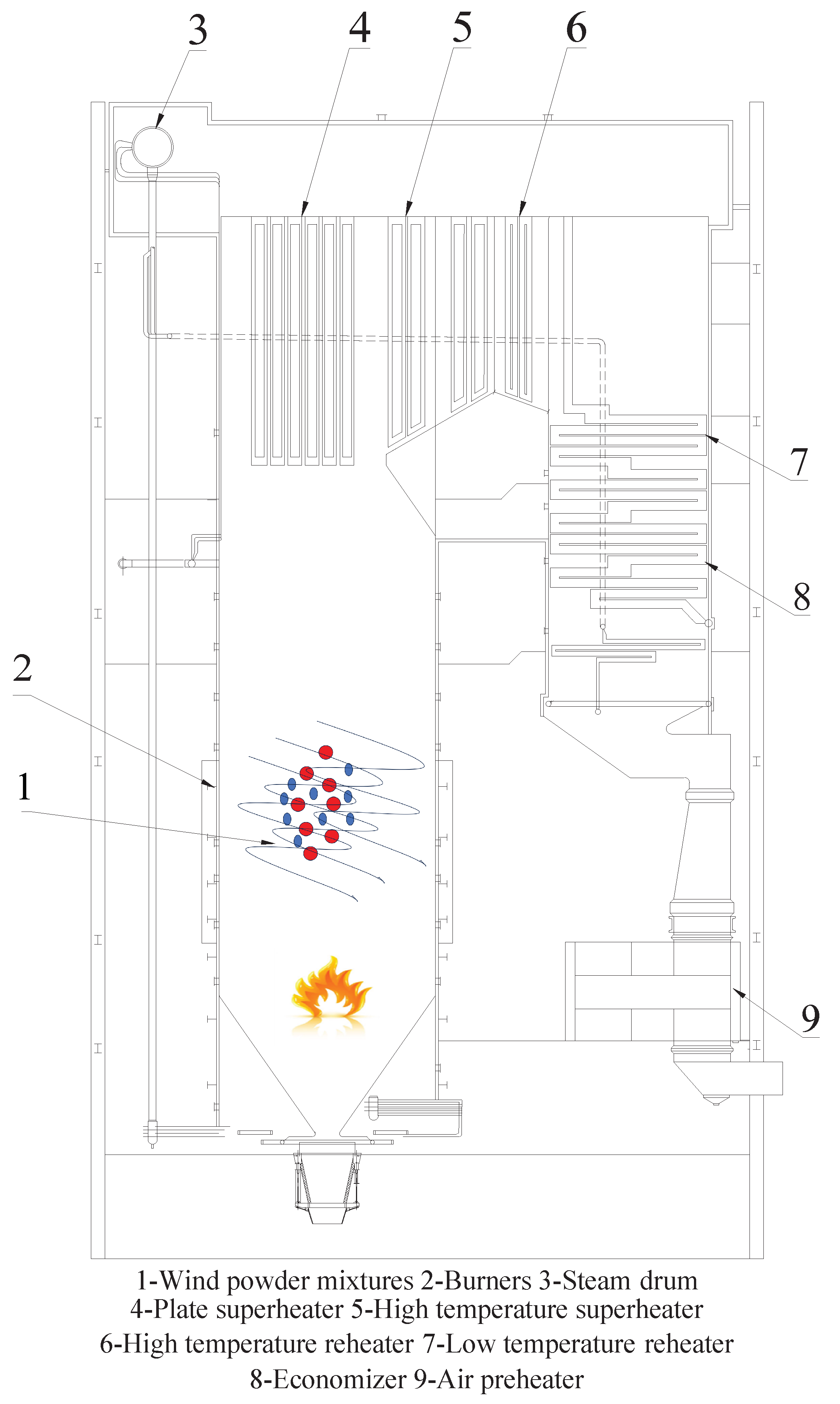
Figure 2.
Economizer internal structure diagram.
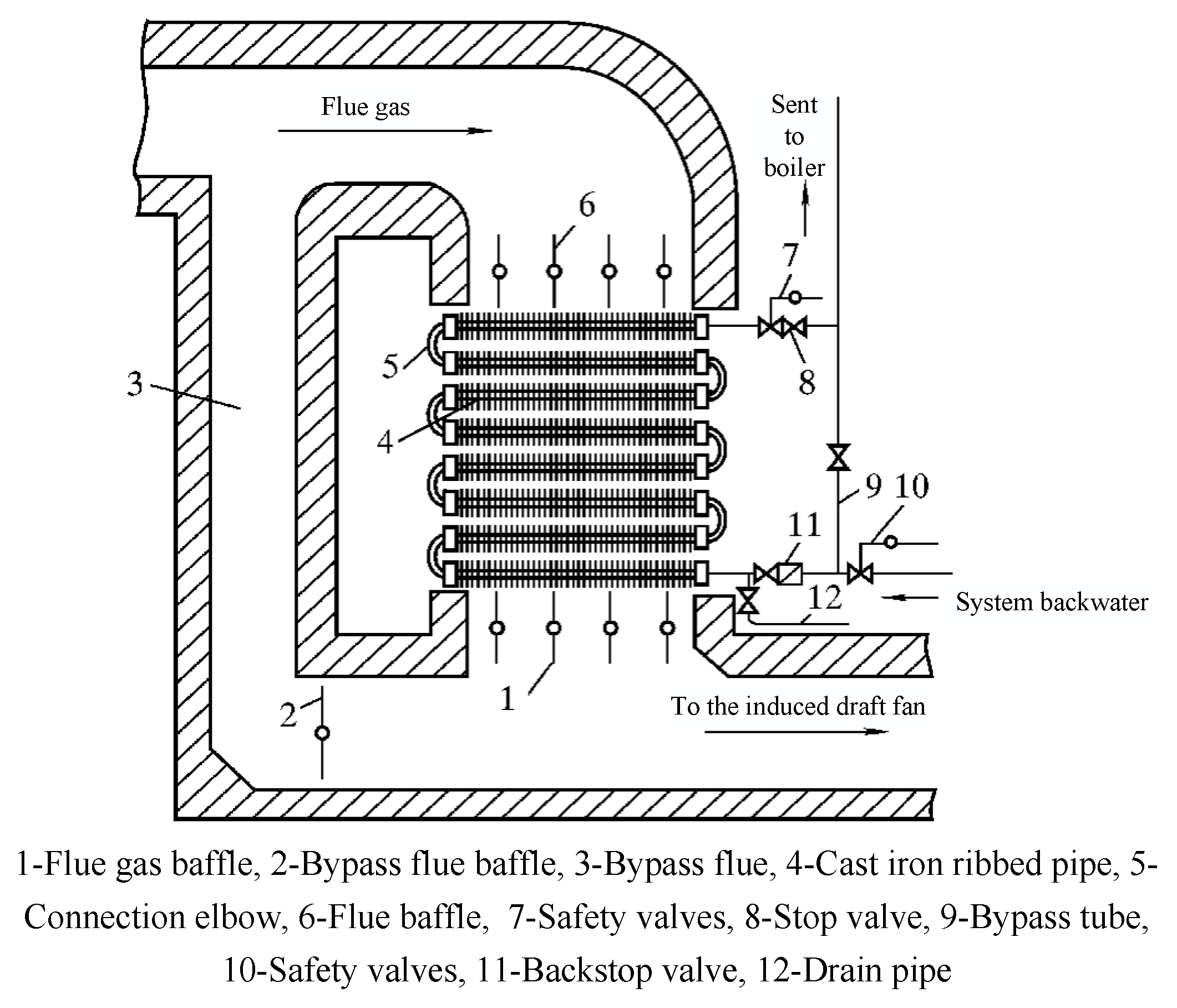
Figure 3.
Schematic of scaling of a single ribbed pipe.
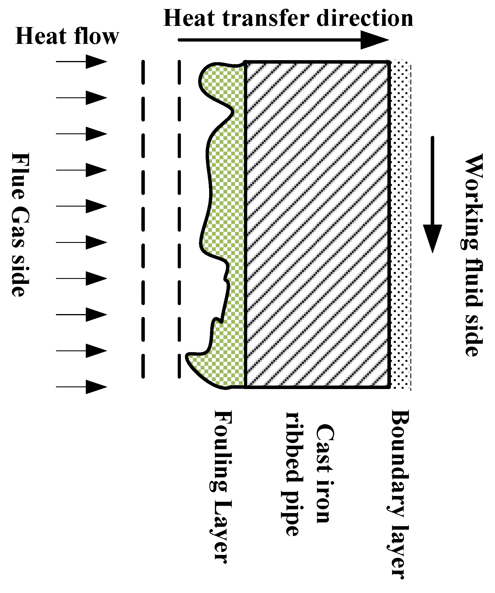
Figure 4.
Cleanliness factor and load variation curves.
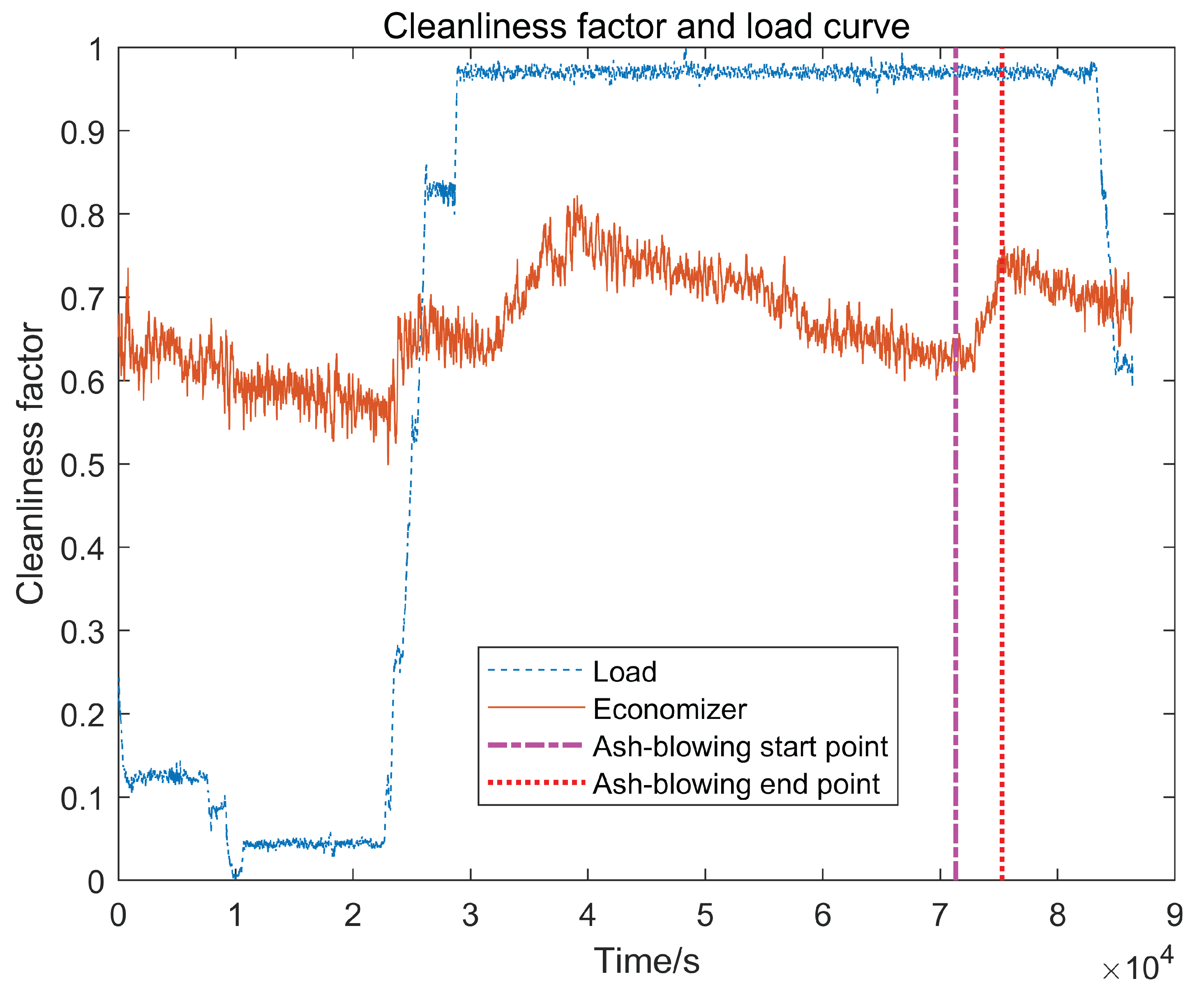
Figure 5.
Economizer cleanliness factor raw data.
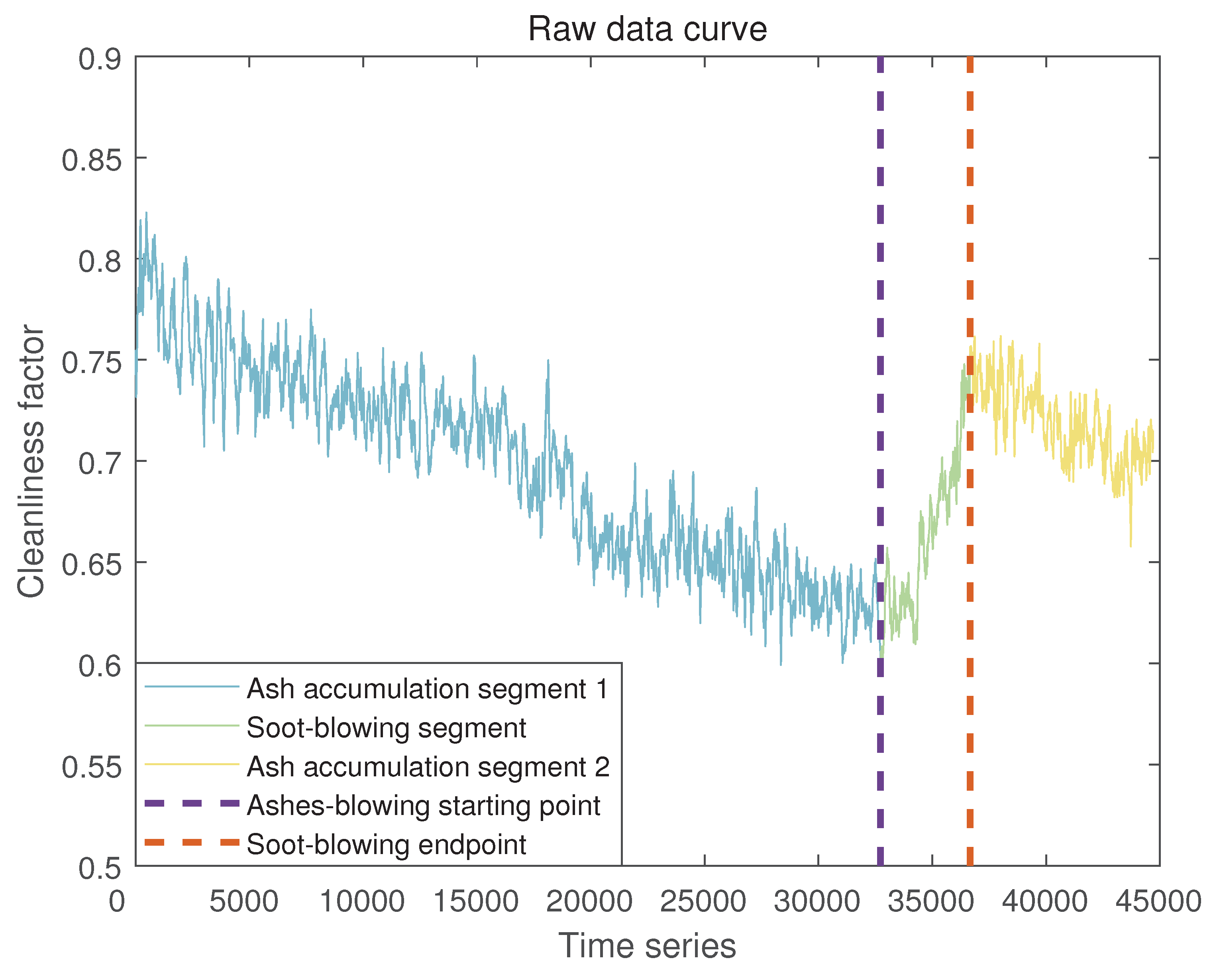
Figure 6.
Comparison of raw data before and after fitting.
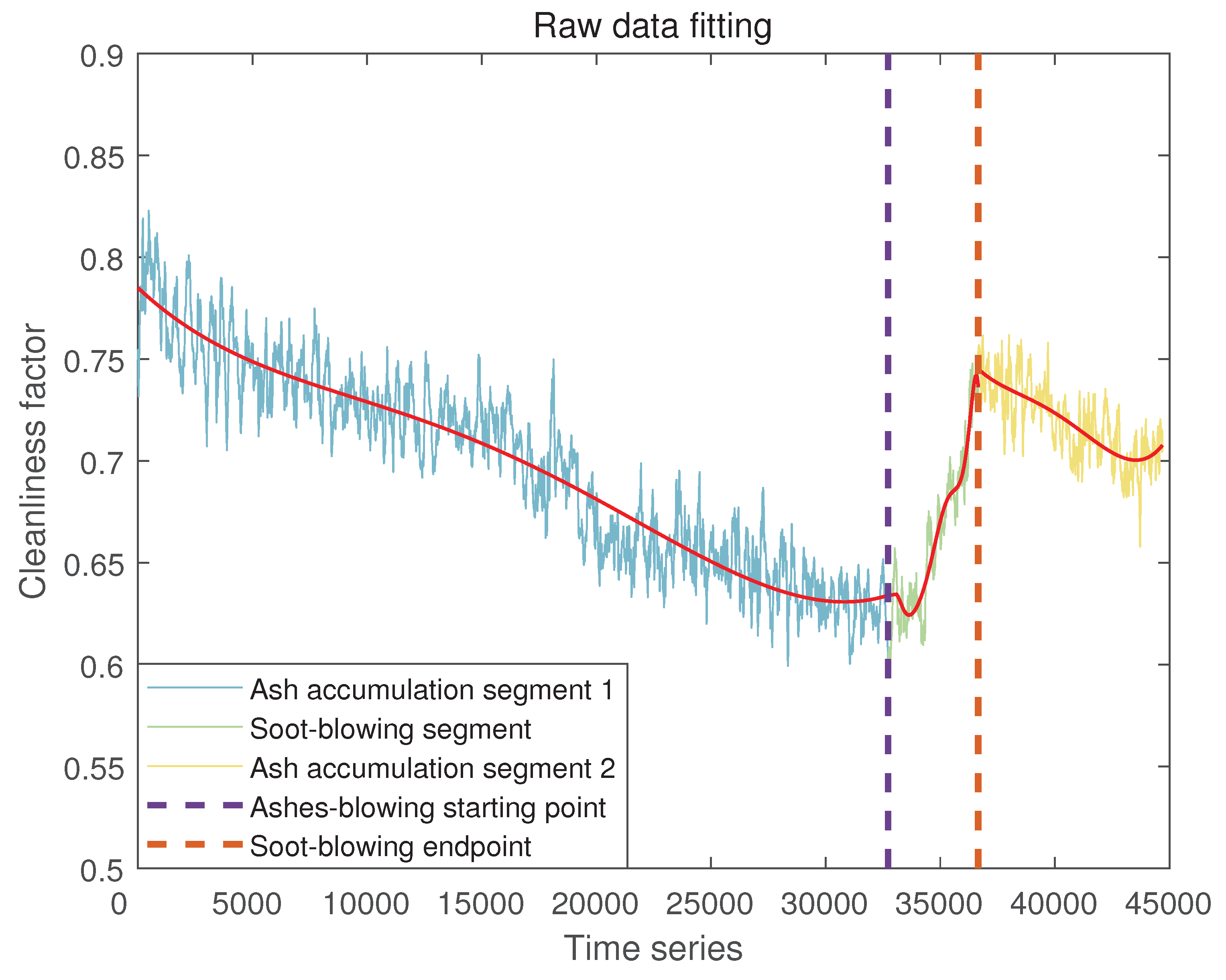
Figure 7.
Heat loss at the heating surface of the economizer.
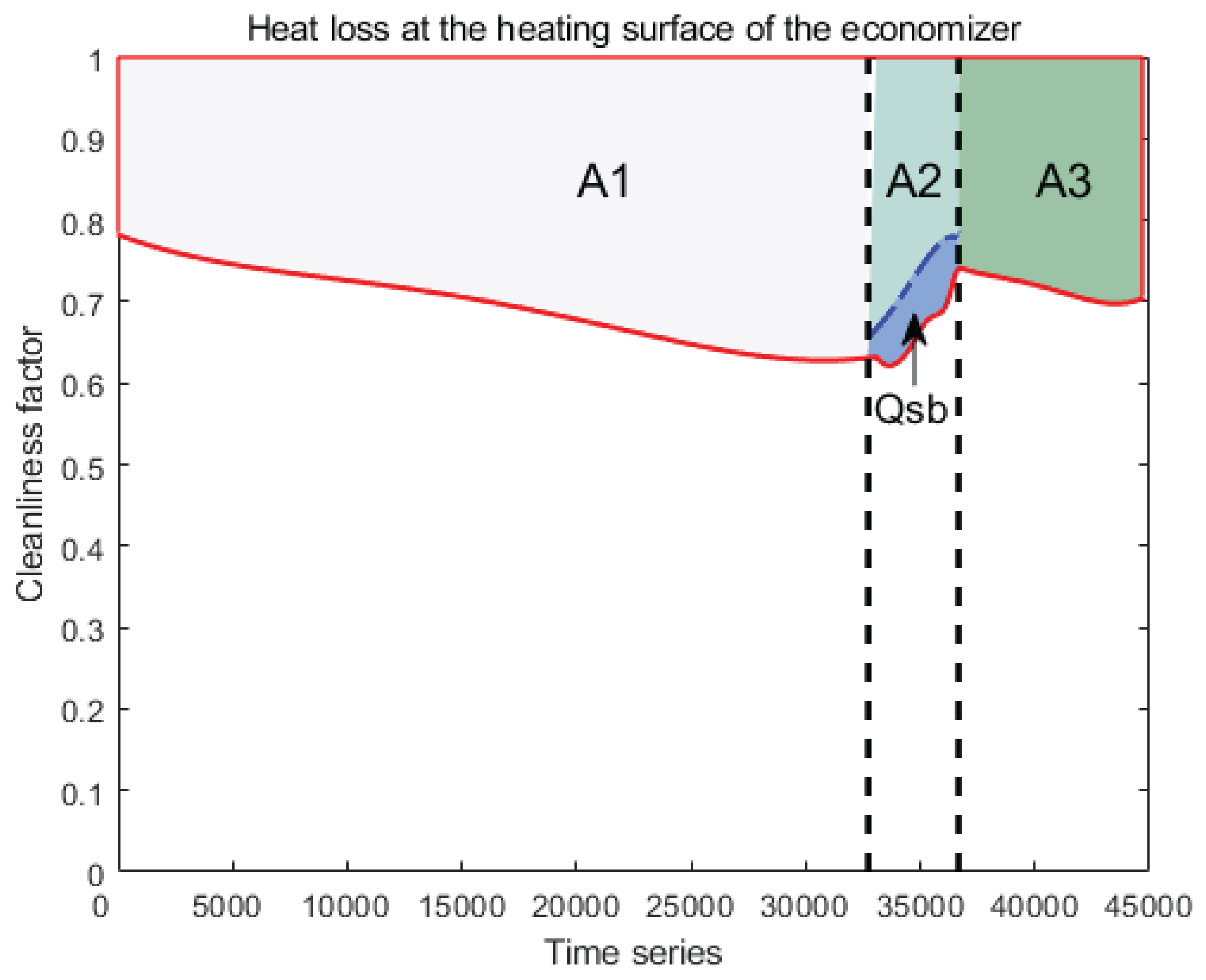
Figure 8.
(a) v-subtraction" extraction phase. (b) v-subtraction" exploratory phase.
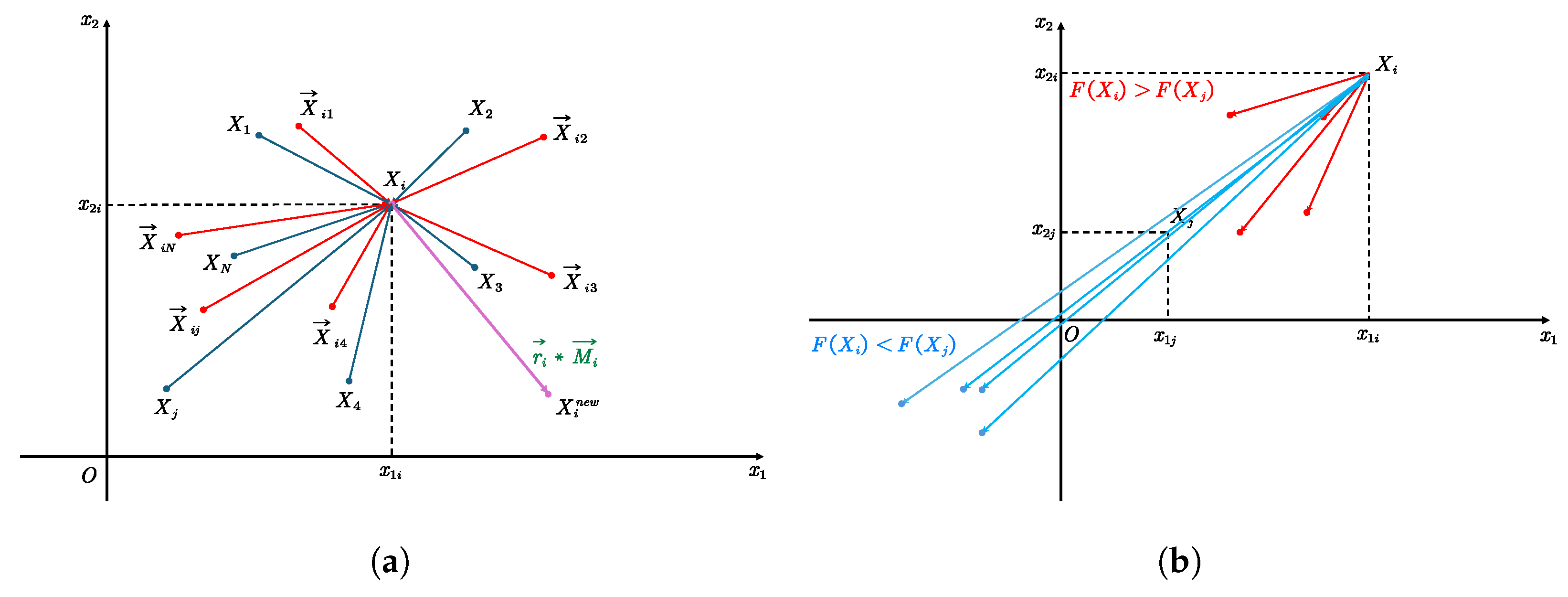
Figure 9.
(a) Distribution of the population after chaotic mapping. (b) Population chaos values and corresponding frequencies.
Figure 9.
(a) Distribution of the population after chaotic mapping. (b) Population chaos values and corresponding frequencies.
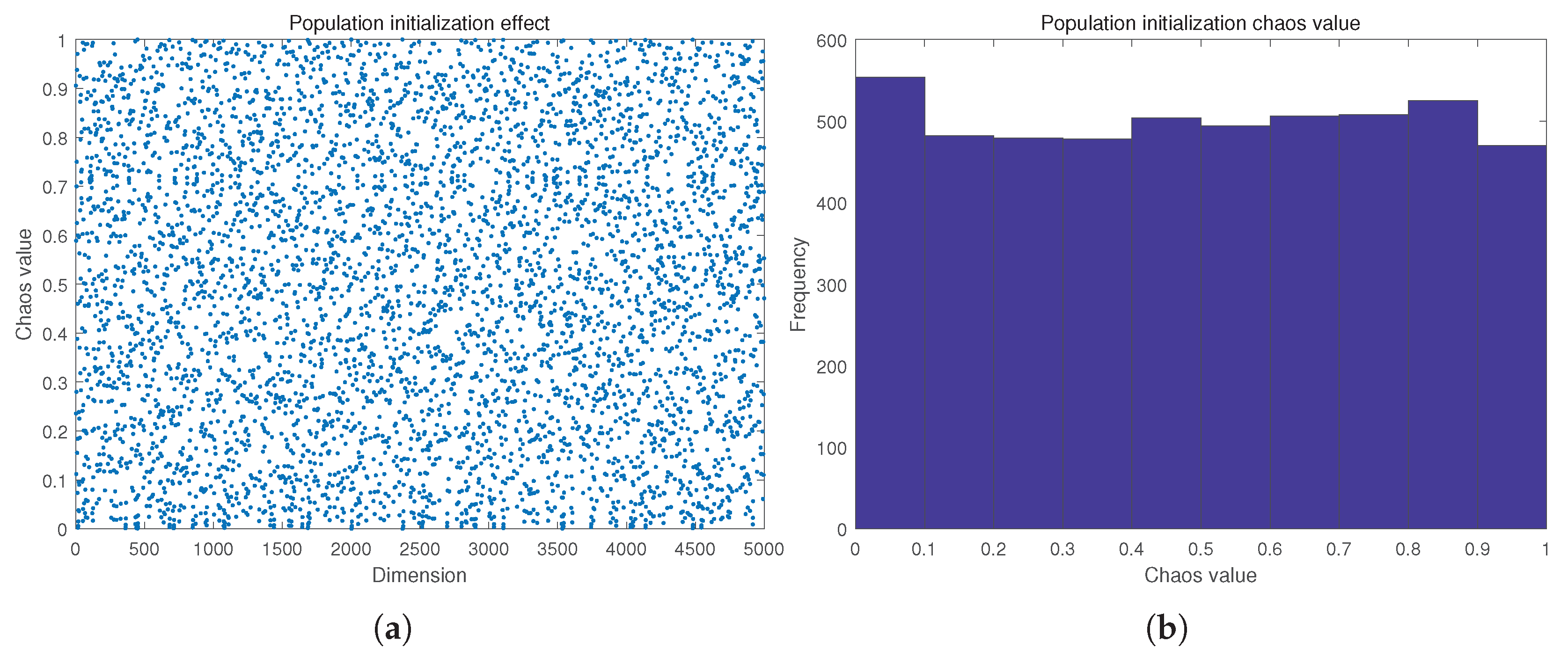
Figure 10.
Schematic diagram of the four independent test roulettes.
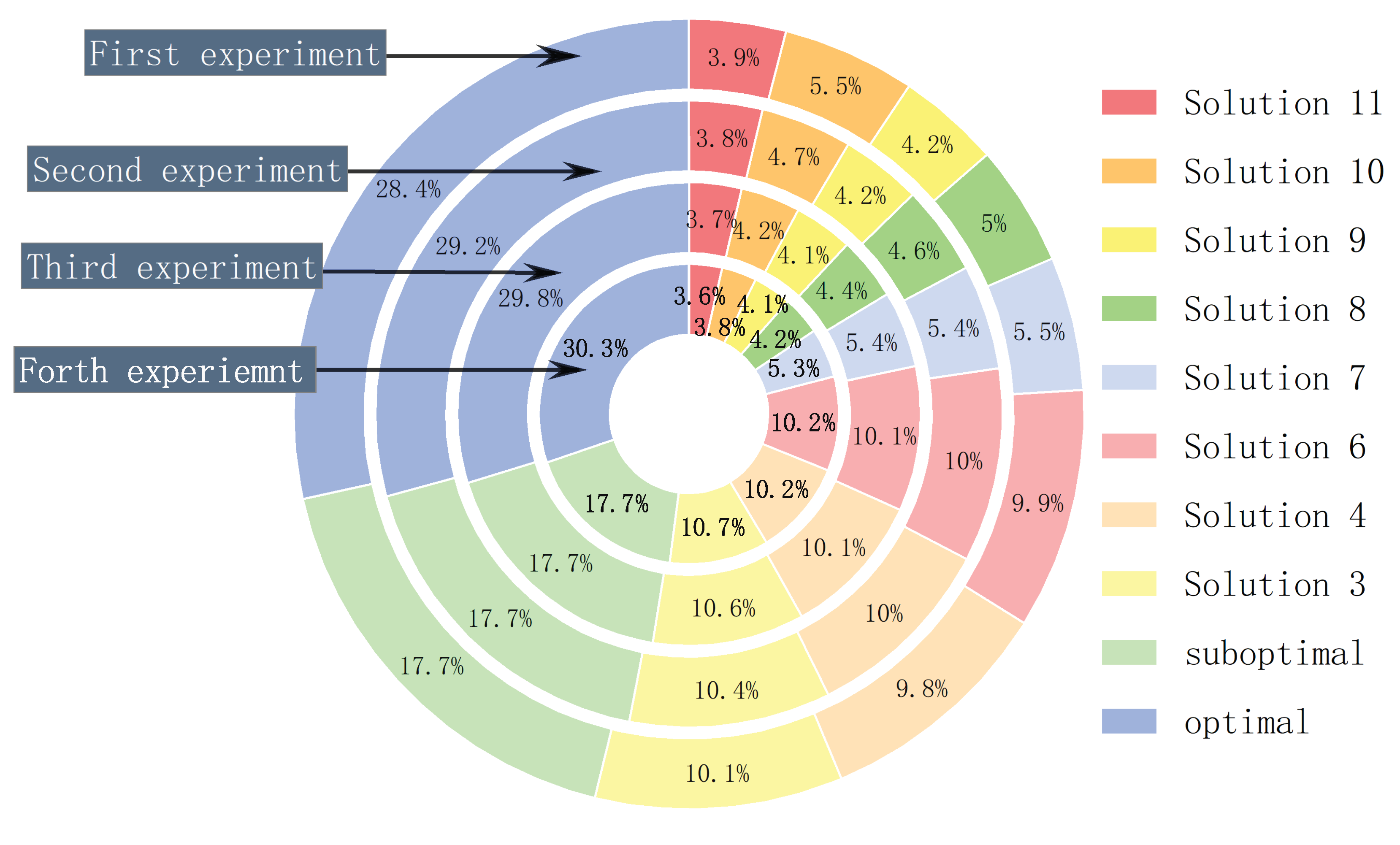
Figure 11.
Schematic of the objective function.
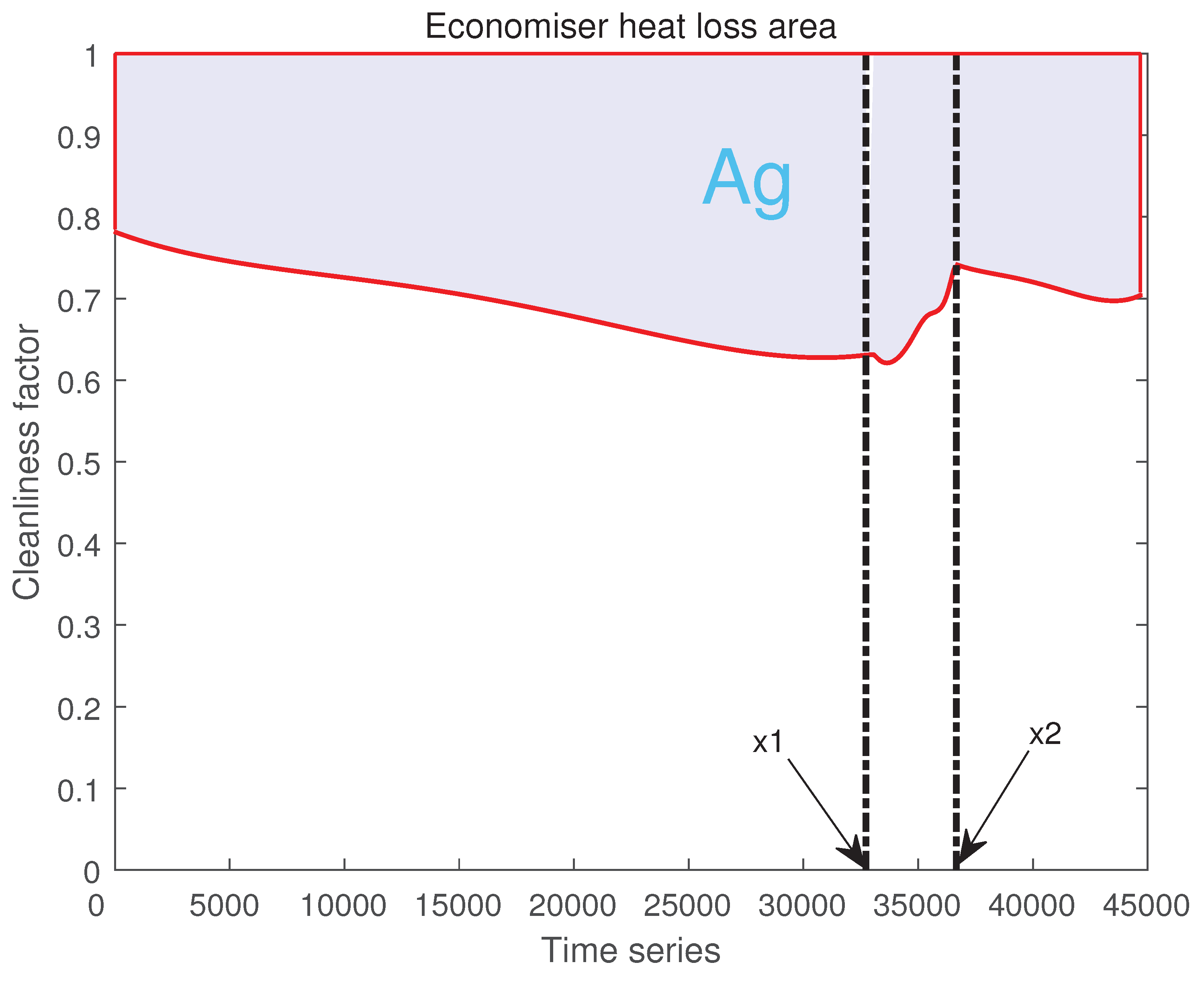
Figure 12.
(a) Soot-blowing starting points calculated by seven optimization algorithms. (b) Soot blowing end points calculated by seven optimization algorithms. (c) Heat loss areas calculated by seven optimization algorithms.
Figure 12.
(a) Soot-blowing starting points calculated by seven optimization algorithms. (b) Soot blowing end points calculated by seven optimization algorithms. (c) Heat loss areas calculated by seven optimization algorithms.
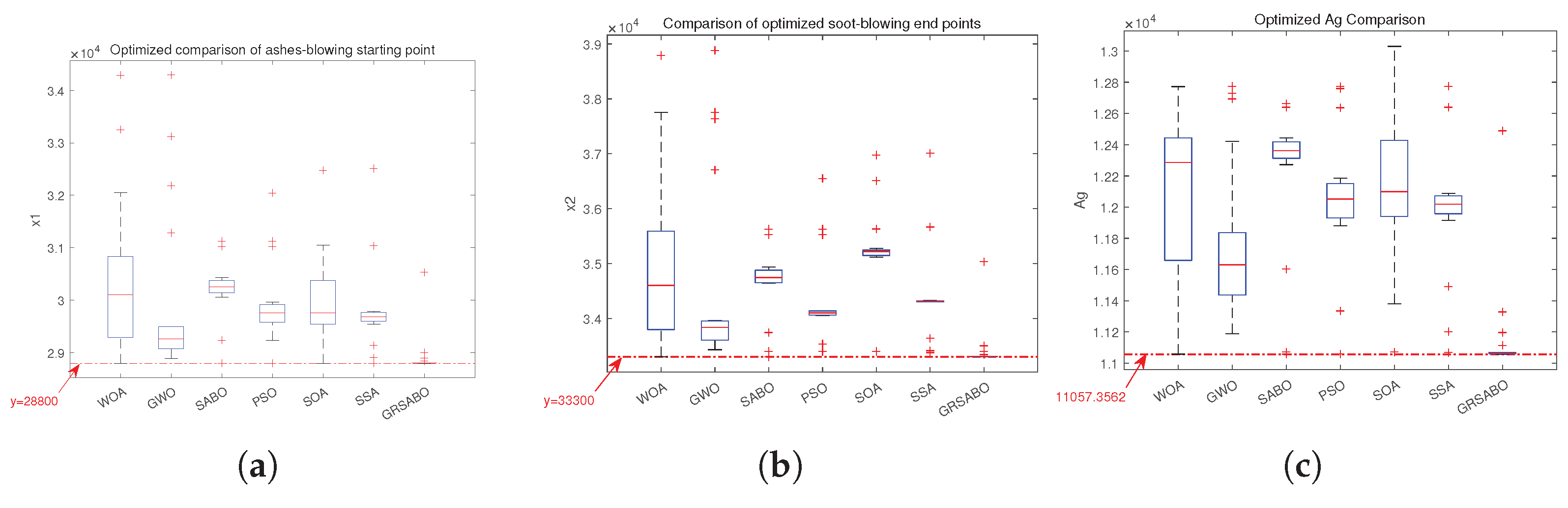
Figure 14.
Structure diagram of GRU model.
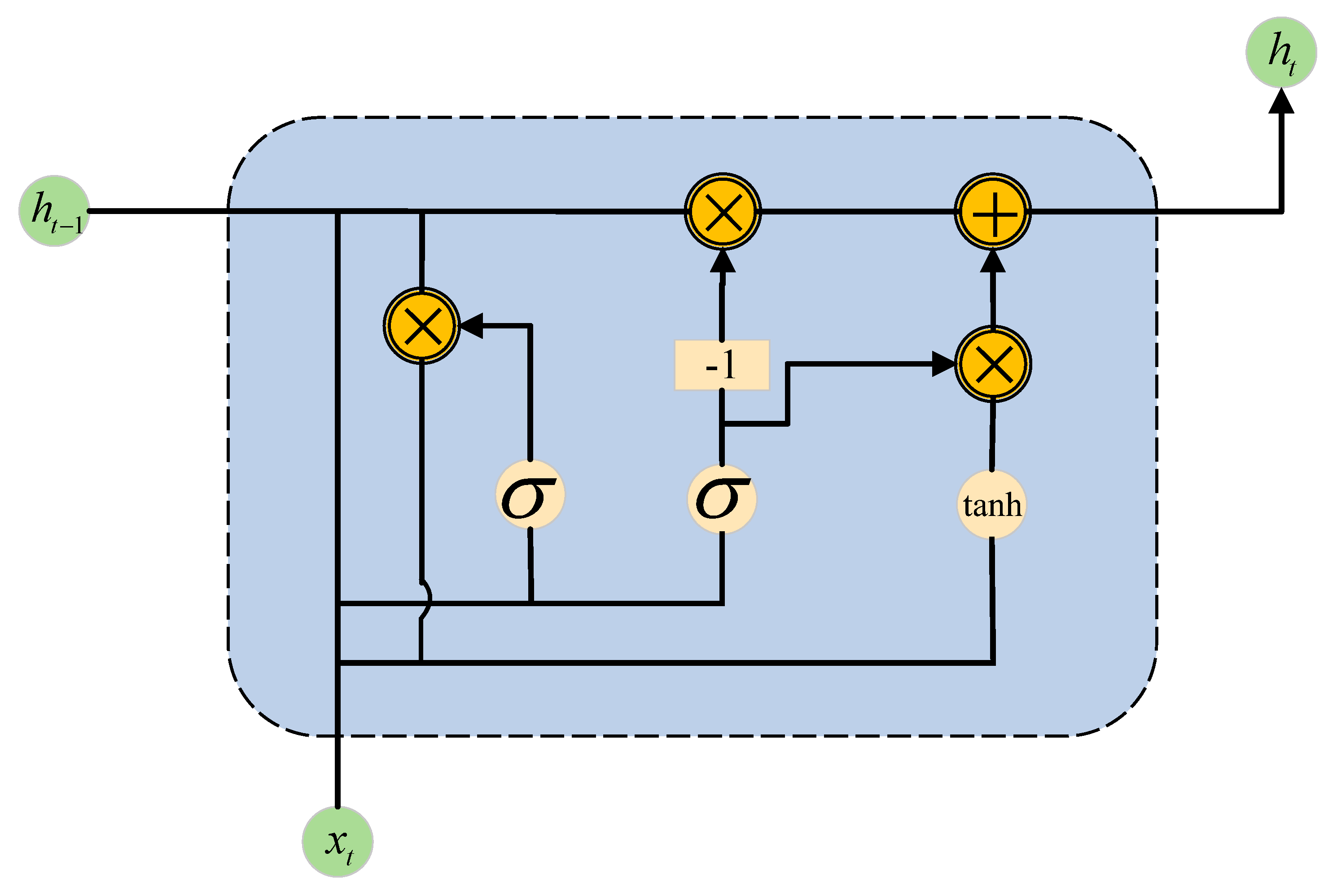
Figure 15.
BiGRU internal structure diagram.
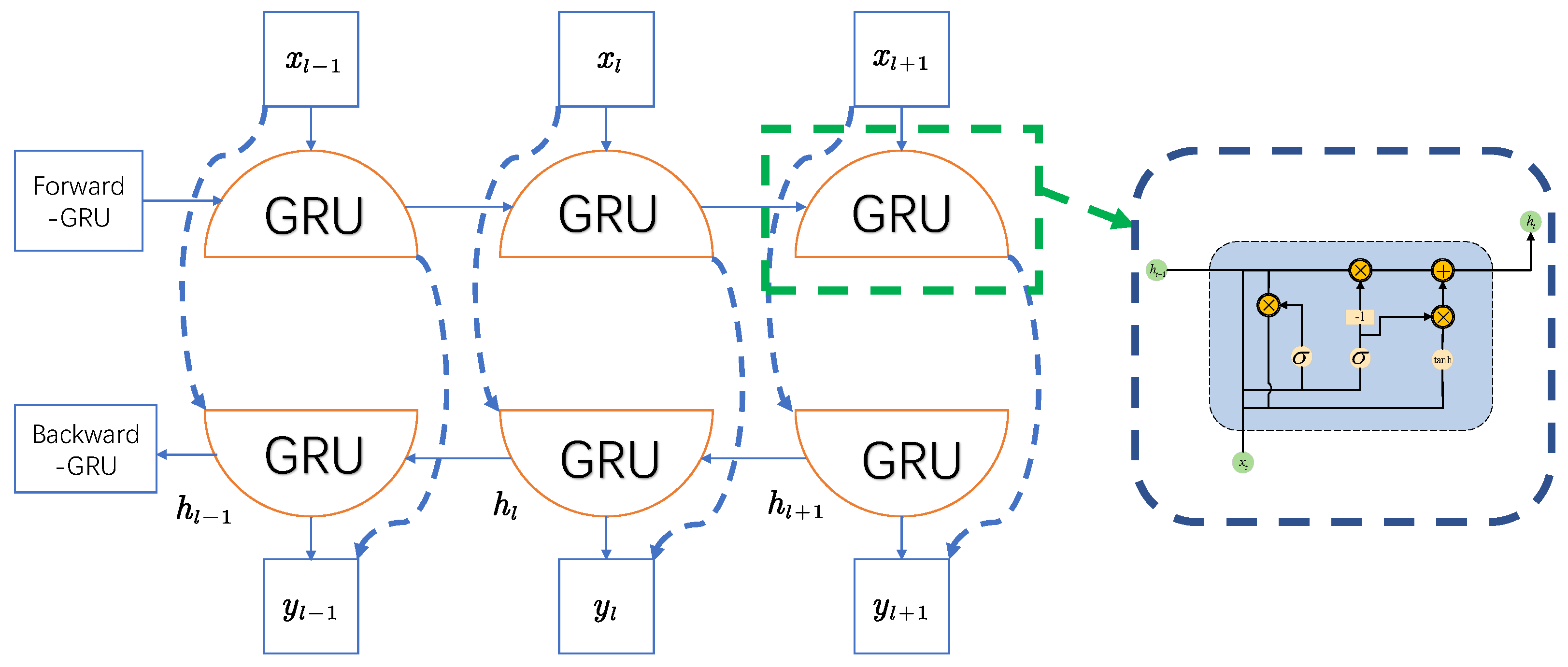
Figure 16.
EEMD-QRBiGRU flowchart.
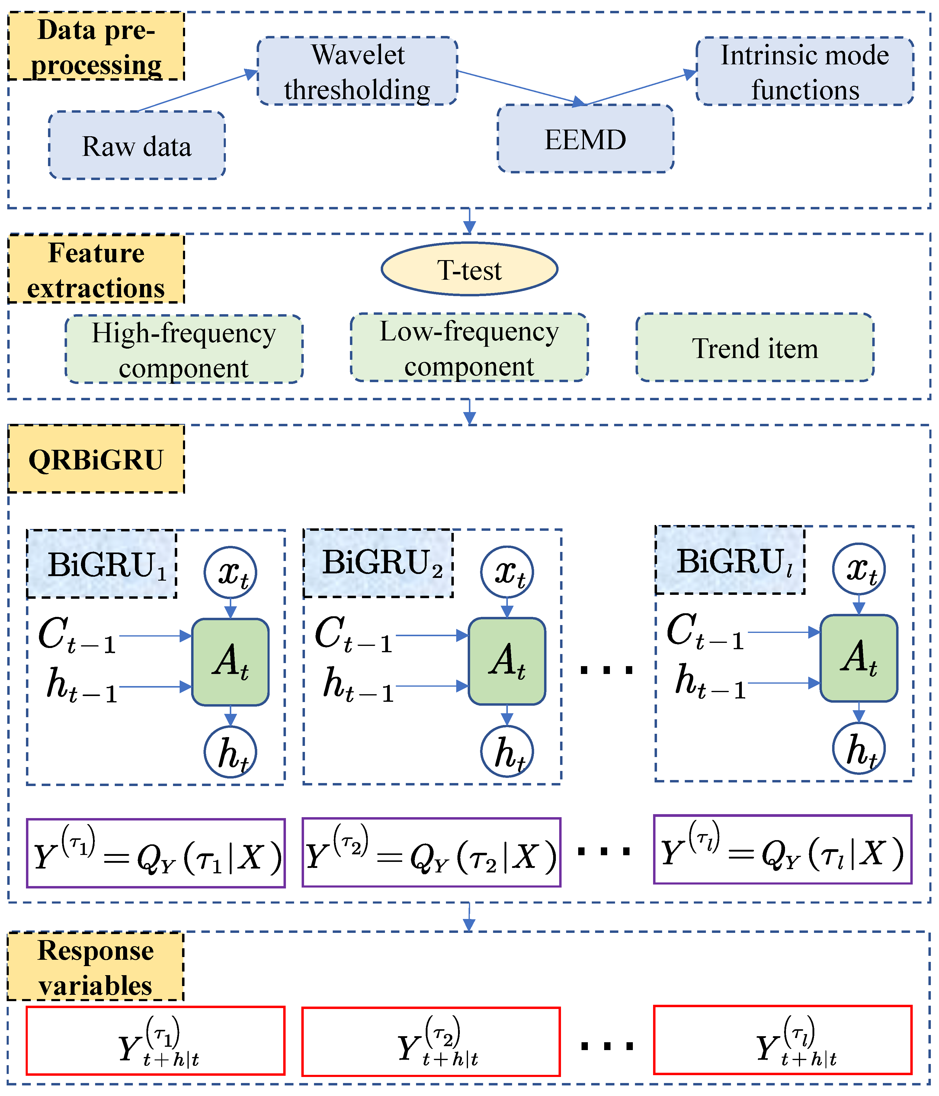
Figure 17.
Comparison of the processing results of four threshold functions.
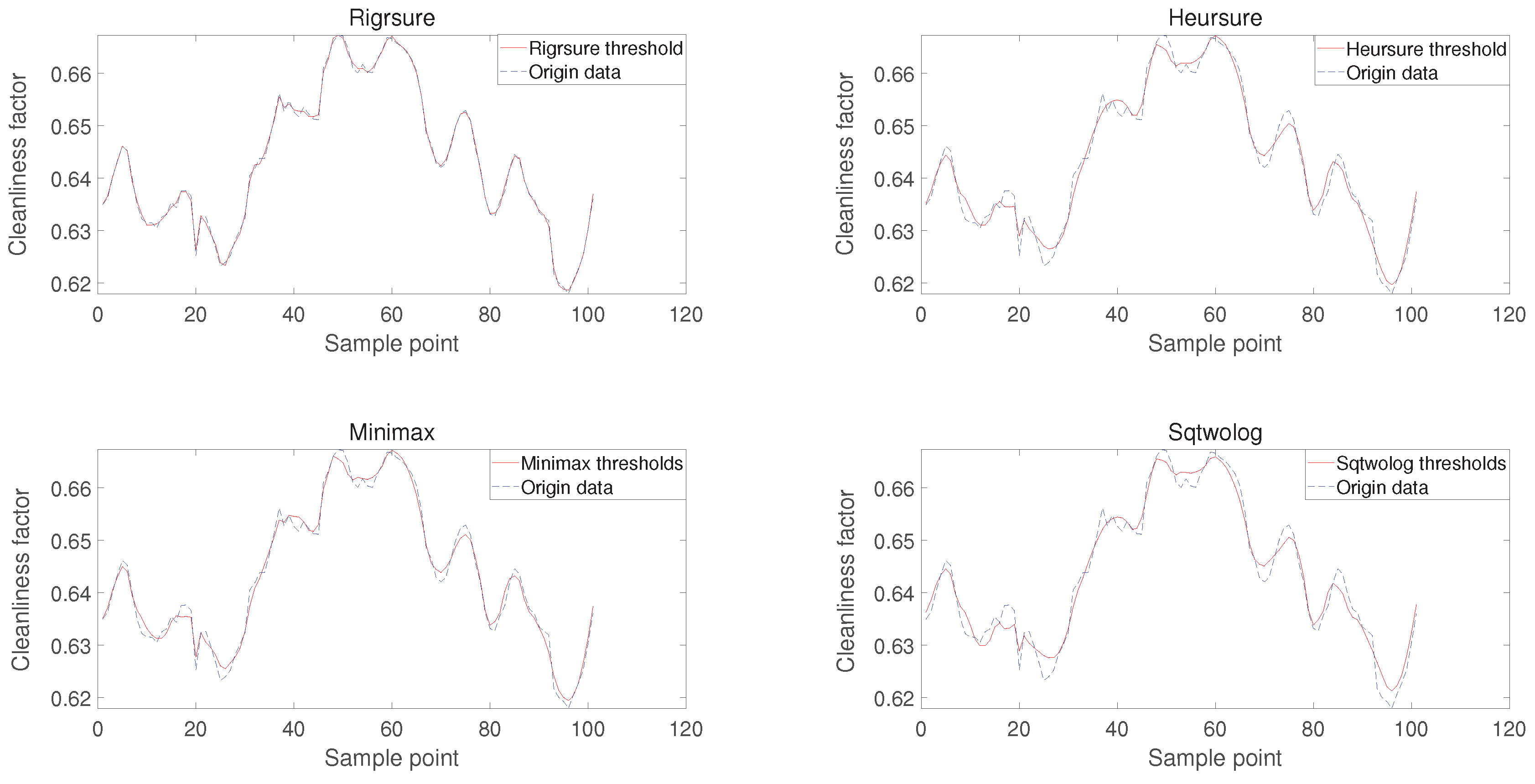
Figure 18.
EEMD decomposition of ash accumulation curve.
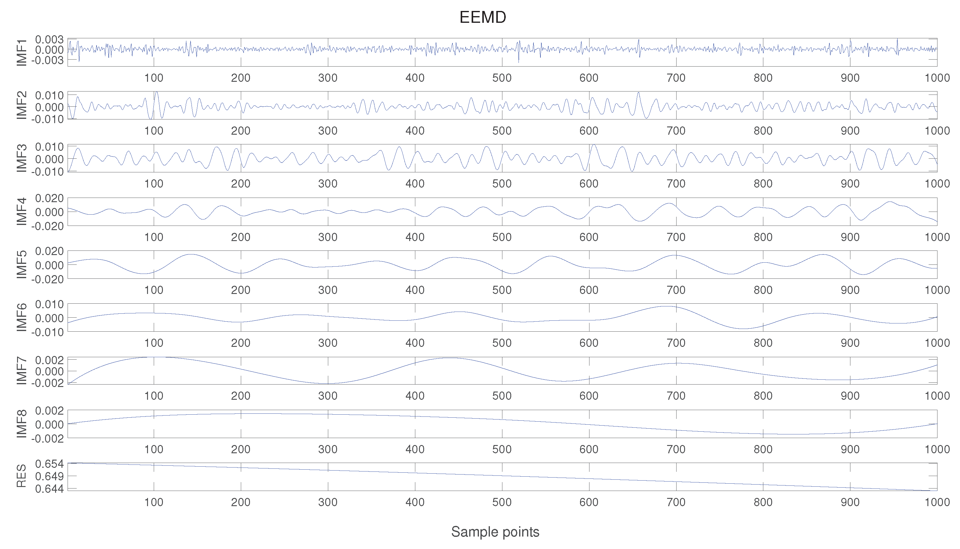
Figure 19.
(a) Test set prediction results. (b) Error histogram. (c) Training set prediction results. (d) Data fitting curve.
Figure 19.
(a) Test set prediction results. (b) Error histogram. (c) Training set prediction results. (d) Data fitting curve.
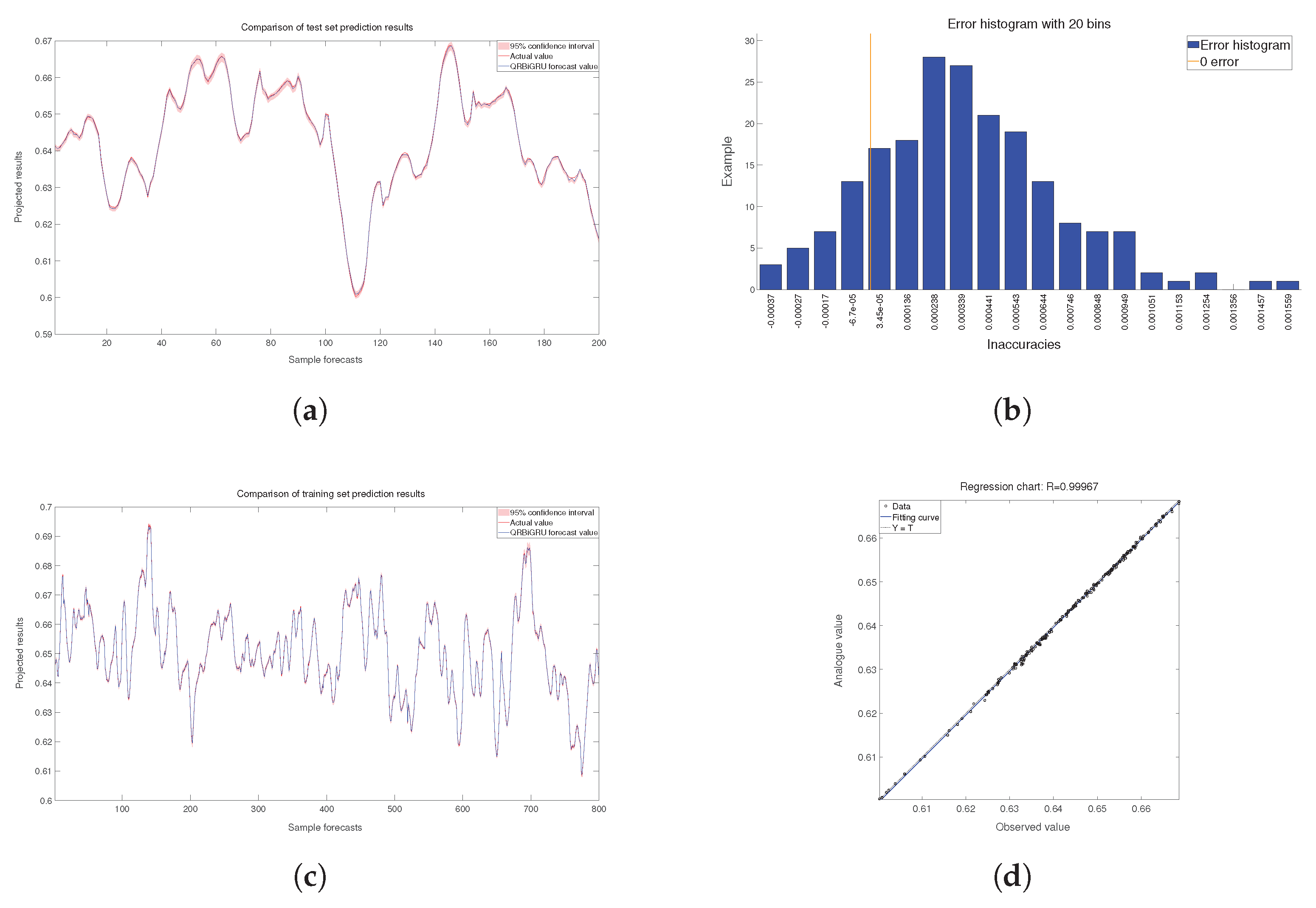
Figure 20.
Comparison of four improved models based on quantile regression.
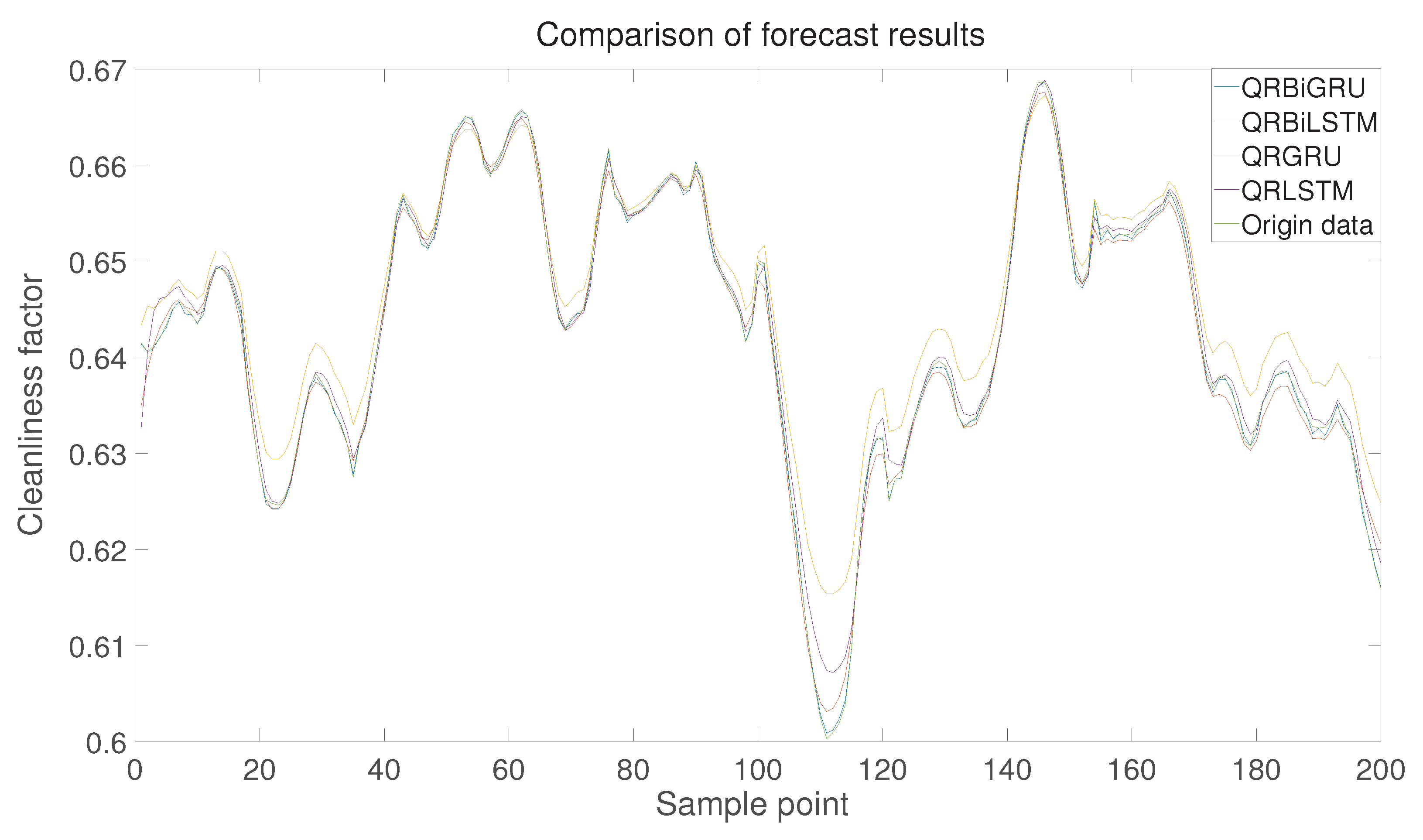
Table 3.
T-value from T-test between indicators.
| Indicator | 1,2 | 2,3 | 3,4 | 4,5 | 5,6 | 6,7 | 7,8 |
|---|---|---|---|---|---|---|---|
| t-value | 0.359666 | 0.65325 | 0.494376 | 0.796583 | 0.353716 | 0.828541 | 1.76e-9 |
Table 4.
Comparison of evaluation indexes related to test set training set.
| Evaluation indicators | Training sets | Test sets |
|---|---|---|
| MAPE | 0.00037 | 0.00046 |
| MSE | 9.431e-08 | 1.437e-07 |
| PICP | 0.96875 | 0.98000 |
| PINAW | 0.00221 | 0.00264 |
Table 5.
This is a wide table.
| Evaluation | QRBiGRU | QRBiLSTM | QRLSTM | |
|---|---|---|---|---|
| MAPE | 0.00046 | 0.00080 | 0.00272 | 0.00149 |
| MSE | 1.437e-07 | 1.923e-06 | 6.534e-06 | 7.279e-07 |
| PICP | 0.98000 | 0.92137 | 0.81546 | 0.92231 |
| PINAW | 0.00263 | 1.99975 | 5.21438 | 3.48572 |
Disclaimer/Publisher’s Note: The statements, opinions and data contained in all publications are solely those of the individual author(s) and contributor(s) and not of MDPI and/or the editor(s). MDPI and/or the editor(s) disclaim responsibility for any injury to people or property resulting from any ideas, methods, instructions or products referred to in the content. |
© 2025 by the authors. Licensee MDPI, Basel, Switzerland. This article is an open access article distributed under the terms and conditions of the Creative Commons Attribution (CC BY) license (http://creativecommons.org/licenses/by/4.0/).
Copyright: This open access article is published under a Creative Commons CC BY 4.0 license, which permit the free download, distribution, and reuse, provided that the author and preprint are cited in any reuse.


