Submitted:
14 July 2025
Posted:
15 July 2025
You are already at the latest version
Abstract
In response to the requirements of advanced aircraft actuation systems for high reliability, high dynamic response, and high-precision control, this paper focuses on the control technology for the master-master working mode of dual-redundancy electro-hydrostatic actuation systems(EHAs). By establishing a multi-domain coupling model that incorporates motor magnetic circuit saturation, hydraulic viscosity-temperature characteristics, and mechanical clearances, a current loop decoupling technique based on vector control is designed. Additionally, adaptive sliding mode control(ASMC) and an improved active disturbance rejection control(ADRC) are combined to enhance the robustness of the speed loop and the disturbance rejection ability of the position loop, respectively. Through the development of a dual-redundancy dynamic model that accounts for hydraulic coupling characteristics, a two-level cooperative control strategy of "position synchronization-current balancing" based on the cross-coupling control(CCC) strategy is proposed to address the challenges of synchronous error accumulation and uneven load distribution in the master-master mode. Experimental results indicate that the control error of the position loop is less than ±0.02 mm, and the load distribution accuracy is improved to over 97%, meeting the design requirements of advanced aircraft. The research findings provide key technical support for the engineering application of power-by-wire flight control systems in advanced aircraft.
Keywords:
dual-redundancy electro-hydrostatic actuation system(EHAs)
; adaptive sliding mode control(ASMC)
; active disturbance rejection control(ADRC)
; master-master working mode
; cooperative control strategy
1. Introduction
With the development of aviation equipment towards intelligence and unmanned operation, flight control actuation systems need to simultaneously meet the requirements of mission reliability (mean time between critical failures less than times/hour) and dynamic performance(position control accuracy less than F.S.) under extreme working conditions [1,2]. Electro-hydrostatic actuation(EHA) systems have become the mainstream solution for advanced aircraft actuation systems due to their advantages of high power density, flexible installation space, and low maintenance costs [3,4,5]. However, single-point failures in a single EHA may lead to flight control failure, and dual-redundancy technology has become the core means to improve reliability through physical redundancy [6,7].
Traditional dual-redundancy systems mostly adopt the "master-standby" working mode, where the standby unit only switches in when the main unit fails [8]. This mode has two major defects [9]: 1) Long-term cold backup of the standby unit causes performance drift of components, prone to dynamic shocks during switching; 2) Only a single system operates under normal conditions, with power capacity utilization of less than . The master-master working mode, through synchronous participation of dual-redundancy units in control, can increase system reliability to over while achieving utilization of power capacity, becoming a key research direction for new-generation civil aircraft [10,11].
The classical control methods commonly used in early flight control actuation systems have struggled to meet the control requirements of electro-hydrostatic actuation systems in terms of steady-state error (1mm) and disturbance rejection capability(0.8mm deviation under ±10kN load fluctuation) [12,13,14]. In recent years, intelligent control algorithms have made progress: The adaptive fuzzy PID control proposed in Ref. [15] improves disturbance rejection accuracy to 0.5mm, but the engineering tuning of the fuzzy rule base takes up to 200 hours; The sliding mode control(SMC) scheme in Ref. [16] enhances robustness through sign function switching, but introduces high-frequency chattering, reducing the service life of hydraulic valves by .
Early studies mostly adopted parallel control strategies based on the rigid shaft hypothesis. For example, Ali et al. [17] achieved position synchronization through dual-closed-loop PI control, but the synchronization error could reach when hydraulic parameters mismatched (such as pump volumetric efficiency deviation >). To address the problem of coupling interference, cross-coupling control (CCC) was introduced [18]. Fan et al. [19] designed a cross-coupling controller based on robust PID, reducing the synchronization error to , but the fixed gain was difficult to adapt to variable load conditions. In recent years, intelligent control algorithms have become a research hotspot. Yao et al. [20] proposed a fuzzy adaptive cross-coupling strategy, which stabilized the synchronization error at under load fluctuation, but the algorithm complexity prolonged the control cycle to 20 ms, exceeding the real-time requirement of no more than 3 ms for flight control actuation systems.
The uneven load distribution in dual-redundancy EHAs is mainly caused by the nonlinearity of hydraulic components (such as the dead zones of pumps/valves) and mechanical installation errors (such as the friction coefficient deviation of hydraulic cylinders exceeding ) [21]. Traditional pressure difference feedback control adjusts load distribution through proportional flow valves. Zhou et al. [22] uses a disturbance observer to compensate for nonlinear factors, controlling the load distribution error within , but the viscosity-temperature variation of hydraulic oil (e.g., -40℃ to +80℃) will lead to mismatch of the compensation model. Sliding mode control is widely applied due to its strong robustness against uncertainties. Hong et al. [23] designs a sliding mode controller, shortening the load error convergence time to 50 ms, but the switching term of the traditional sign function easily causes high-frequency chattering, aggravating the wear of hydraulic valves.
The dual-redundancy EHA system proposed in this paper achieves performance breakthroughs through deep integration of mechanical, electrical and hydraulic systems and control coupling:
Physical-layer redundancy: two independent "motor-pump-sensor" channels (electrical isolation > 100M) realize force synthesis through coaxial drive of the actuator, with mechanical structure stiffness increased by compared to single-channel systems.
Control-layer collaboration: in the master-master working mode, dual channels synchronously track commands, with load sharing error less than , which is lower than that of the master-standby mode.
Enhanced mission reliability: the fault monitoring matrix significantly improves the system’s mission reliability.
Aiming at the existing technical gaps, a technical system of "model precision-control stratification-verification engineering" is constructed, with the core innovations as follows:
Speed loop: a fuzzy sliding mode composite controller is designed to solve the problems of inertia time-varying and friction nonlinearity in the pump control system.
Position loop: the improved Active Disturbance Rejection Control(ADRC) introduces a dynamic compensation factor to achieve real-time suppression of load interference.
Main innovations in master-master control strategy are as follows:
- 1.
- A two-level collaborative algorithm of "position synchronization-current balancing" is studied, with the position synchronization error time <3ms.
- 2.
- Dynamic synchronization technology: A high-precision dual-channel synchronization error monitoring model is established. Combined with 40 Mbps high-speed communication and a 100 ultra-short synchronization period, real-time error capture is realized. A phase compensation dynamic adjustment mechanism is innovatively introduced to effectively eliminate the displacement cumulative error caused by the phase difference, ensuring the accuracy of system operation.
- 3.
- Adaptive load balancing strategy: The causes of load imbalance such as hardware, control delay, and external interference are deeply analyzed. An intelligent current loop balancing algorithm based on deviation coupling is designed to achieve dynamic optimization of torque commands. By integrating hydraulic pressure feedforward compensation technology, a closed-loop feedback regulation system is constructed, significantly improving the load sharing accuracy and the system’s anti-interference ability.
2. Multi-Domain Coupling Modeling of Electro-Hydrostatic Actuation System
2.1. Construction of Precision Model for Permanent Magnet Synchronous Motor (PMSM)
2.1.1. Coordinate Transformation Considering Saturation Effect
Based on the traditional Clark/Park transformation, a magnetic circuit saturation correction coefficient is introduced to establish a nonlinear inductance model:
where and are unsaturated inductances, and , are saturation coefficients obtained by finite element simulation fitting.
2.1.2. Coupling Model of Iron Loss and Copper Loss
The total motor loss is , where the copper loss is , and the iron loss is . The iron loss equivalent current satisfies:
2.2. Hydraulic-Mechanical Coupling Model of EHA Actuator
2.2.1. Variable-Viscosity Hydraulic Flow Model
Considering the variation of oil viscosity with temperature (, where T is the oil temperature in °C), the actual output flow is corrected as:
where is the volumetric efficiency at 25°C, and is the temperature influence coefficient, which improves the modeling accuracy by 18
2.2.2. Actuator Cylinder Dynamics with Clearance Nonlinearity
Considering the nonlinear force caused by the clearance between the piston and cylinder, a piecewise model is established:
where is the clearance stiffness, is the clearance amount. The Coulomb friction force is fitted by the Stribeck curve as , which better approximates the actual friction characteristics.
3. Engineering Design Architecture of Dual-Redundancy Electro-Hydrostatic Actuation System
3.1. Architecture of Electro-Hydrostatic Actuator
The electro-hydrostatic actuator is an electrical-mechanical-hydraulic dual-redundancy system. System I and System II of the actuator are respectively connected to the two chambers of a series actuator cylinder. Under normal conditions, both systems operate in a master-master configuration, jointly outputting displacement and pressure to drive the load. If any system fails, it will be bypassed while the other system continues to operate normally, putting the actuator in a fail-operational state. After both systems fail, the actuator will move to the neutral position under the action of an external pneumatic load and achieve hydraulic locking, entering a fail-safe state. A permanent magnet synchronous motor drives a bidirectional hydraulic pump to rotate. The output flow of the hydraulic pump, in accordance with the motor’s speed and direction, directly controls the position, speed, and direction of the actuator cylinder. An accumulator serves as the oil tank of the electro-hydrostatic actuator, compensating for temperature changes and providing backpressure to the hydraulic pump. Solenoid valves and mode valves together accomplish the mode of the actuator. High-pressure sensors are used to monitor the pressure in the two chambers of the hydraulic pump, calculate the magnitude of the load force, and conduct fault monitoring. A low-pressure sensor with temperature measurement monitors the accumulator pressure and oil temperature. The structure of the dual-redundancy electro-hydrostatic actuator is shown in Figure 1.
3.2. Architecture of Actuator Controller
The controller consists of an electronic control unit and a power drive unit. The electronic control unit implements functions such as redundancy management, motor drive algorithms, signal input/output conditioning, and bus data processing, while the power drive unit realizes functions such as power driving. The structure of the actuator controller is shown in Figure 2.
4. Control Algorithm Design
4.1. Current Loop Vector Control and DQ-Axis Decoupling Technology
4.1.1. Vector Control and Coordinate Transformation
The core of vector control is to convert a three-phase AC motor into an equivalent DC motor model through coordinate transformation, enabling independent control of excitation current and torque current. The specific transformation process is as follows:
Clark Transformation (abc→) converts voltages/currents in the three-phase stationary coordinate system to a two-phase stationary coordinate system:
Park Transformation (→dq) converts to a synchronous rotating coordinate system via the rotor position angle :
where , p is the number of pole pairs, is the mechanical angle, and is the initial electrical angle.
4.1.2. DQ-Axis Voltage Equation and Decoupling Control
In the synchronous rotating coordinate system, the voltage equation of PMSM is:
It can be seen that the dq-axis voltages have cross-coupling terms ( and ). To achieve decoupling, a feedforward compensator is designed to eliminate the coupling terms, yielding the decoupled voltage commands:
By real-time measuring the electrical angular velocity and feedback currents , the cross-coupling effects can be dynamically compensated to achieve independent dq-axis control.
4.1.3. Current Loop Control Law Design
The current loop is designed with a Proportional-Integral (PI) controller, and the control law is:
where and are the PI controller parameters for the dq-axis. Parameters are determined by the pole placement method to make the current loop bandwidth reach 1000Hz, meeting the requirement for fast dynamic response.
4.1.4. Voltage Vector Synthesis Based on SVPWM
The seven-segment SVPWM modulation technique is adopted to generate inverter drive signals, with a voltage utilization rate of over . The specific steps are as follows:
- Sector judgment: determine the sector based on the -axis voltage vector coordinates, and use the sign judgment method to control the sector judgment time within ;
- Vector action time calculation: calculate the action times of the basic voltage vectors and the zero vector action time according to the volt-second balance principle;
- Switching sequence generation: arrange the switching states according to the principle of "zero vector symmetry" to reduce switching losses, with a typical switching frequency set to 20kHz.
4.1.5. High-Speed Flux-Weakening Control Strategy
When the motor speed exceeds the base speed, the speed regulation range is expanded through flux-weakening control. The flux-weakening criterion is defined as:
The excitation current command under flux-weakening control is:
where the exponential factor n is the flux-weakening intensity coefficient. The is adjusted in real-time through a flux observer to suppress back EMF saturation, enabling the flux-weakening speed regulation range to reach 2.0 times the rated speed.
4.2. Adaptive Sliding Mode Control for Speed Loop
4.2.1. Basic Theory of Sliding Mode Control
Sliding Mode Control (SMC) forces the system state to converge to a preset sliding surface within a finite time by designing a discontinuous control law, and performs sliding motion along the sliding surface, which has inherent robustness to parameter perturbations and external disturbances. For the speed loop control object, the speed error is defined as , where is the speed command and is the actual speed. The sliding surface is designed as:
When the system state reaches the sliding surface (), the sliding condition is satisfied. At this time, the dynamic characteristics are determined by the sliding surface equation, independent of system parameters, achieving decoupling control for uncertainties.
4.2.2. Design of Adaptive Sliding Mode Controller
Aiming at the time-varying moment of inertia (such as ) and friction nonlinearity (combined action of Coulomb friction and viscous friction) of the pump-controlled electro-hydrostatic actuation system, an Adaptive Sliding Mode Controller (ASMC) is designed. The speed loop takes the output by the current loop as the control quantity, and the control law is divided into two parts: equivalent control and switching control :
1. Equivalent Control Law (Handling Matched Uncertainties)
Assuming the system is on the sliding surface (), the equivalent control quantity can be obtained from the sliding surface equation:
where is the motor torque coefficient, is the load torque, and B is the viscous damping coefficient. In practical applications, since J and are unknown, they need to be estimated online through an adaptive mechanism.
2. Switching Control Law (Handling Mismatched Uncertainties)
To force the system state to converge to the sliding surface quickly, a switching control term is designed:
where is a saturation function (replacing the traditional sign function to suppress chattering):
where is the boundary layer thickness (such as ), and is the switching gain, which is dynamically adjusted by an adaptive law to adapt to load changes.
4.2.3. Implementation of Adaptive Mechanism
To cope with the strong uncertainties of the moment of inertia J (variation range ) and load torque (fluctuation ) in the pump-controlled electro-hydrostatic actuation system, a fuzzy logic-based adaptive algorithm is designed to improve the robustness of the sliding mode controller by online adjusting control parameters. This mechanism includes four core links: input fuzzification, rule base construction, fuzzy inference, and defuzzification, which are implemented as follows:
Considering the uncertainties of the moment of inertia J and load torque , a fuzzy logic adaptive algorithm is introduced to adjust control parameters online:
1. Processing of input variables and universe of discourse mapping
We define the mapping from physical quantities to the fuzzy universe of discourse. The speed error () and error change rate () are defined as input variables, which are mapped from the physical domain to the fuzzy universe through quantization factors :
where the quantization factors are determined according to the maximum working conditions: - , 1.5 times the rated speed; - , the maximum angular acceleration. Then carry out the division of the fuzzy universe of discourse. Five symmetric fuzzy subsets are used to describe the input variables: NB (Negative Large), NM (Negative Medium), ZO (Zero), PM (Positive Medium), PB (Positive Large), and the membership function uses a Gaussian type:
where the central value , and the width parameter , ensuring the subset overlap is about to balance control sensitivity and stability.
2. output variable design and scale factors.
The output variables are the switching gain (affecting the chattering intensity) and the sliding mode coefficient (determining the slope of the sliding surface), which are mapped from the fuzzy universe to the physical domain through scale factors :
where (unit: V/A) is determined according to the voltage withstand of power devices and motor characteristics; (unit: ) matches the system bandwidth through frequency domain analysis.
3. Construction of Fuzzy Control Rule Base Based on Lyapunov stability theory and engineering debugging experience, a total of 49 control rules in 5×5 are established. The core rule design principles are as follows:
- Error-Dominated Rules:
- when is PB, increase to reduce the error quickly, and increase to improve the response speed;
- Error Change Rate-Dominated Rules:
- when is NB (the error decreases rapidly), decrease to prevent overshoot;
- Rules Near Zero Error:
- when both and are ZO, use medium gain to maintain steady-state accuracy.
Typical rules are shown in the following table.

Table 1.
Example of typical rules.
| Rule Number | Condition (IF) | Conclusion (THEN) |
|---|---|---|
| 1 | is NB and is NB | is NB, is NB |
| 25 | is ZO and is ZO | is ZO, is ZO |
| 49 | is PB and is PB | is PB, is PB |
The rule base satisfies symmetry (mirror response for positive/negative errors) and completeness (covering all input combinations), and passes consistency checks to ensure no conflicting rules.
4. Fuzzy Inference and Defuzzification
Mamdani-type inference is used, and the rule activation degree is calculated by the "minimum method":
where are the membership degrees of the input variables to each fuzzy subset.
The weighted average of the output fuzzy set is used to obtain the precise control quantity:
where is the discrete point of the output universe (such as 101 uniformly sampled points), and is the corresponding membership degree. This method has low computational complexity (e.g., single-cycle calculation takes <1), suitable for embedded real-time control.
Through the above design, the fuzzy logic adaptive mechanism realizes the dynamic optimization of sliding mode control parameters, enabling the speed loop to have both fast response capability and strong robustness under complex working conditions, laying the foundation for high-precision position loop control. This method can be extended to the adaptive adjustment of control parameters for other nonlinear and uncertain systems.
4.2.4. Chattering Suppression and Stability Analysis
The high-frequency chattering of traditional sliding mode control will aggravate the wear of the hydraulic system. The following measures are taken to suppress it:
- Boundary layer design:
- replace the sign function with a saturation function to limit the chattering amplitude within the boundary layer ();
- Low-pass filtering:
- first-order filtering (such as cutoff frequency 500Hz) is performed on the switching control output to reduce high-frequency components;
- Adaptive adjustment:
- dynamically adjust according to the speed error to avoid chattering caused by excessive gain.
In terms of stability, it is proved by the Lyapunov function:
where and are parameter estimation errors. When the sliding condition is satisfied, , and the system state eventually converges to the neighborhood of the sliding surface, ensuring the asymptotic stability of the closed-loop system.
4.3. Improved Active Disturbance Rejection Control for Position Loop
Active Disturbance Rejection Control (ADRC), proposed by researcher Han Jingqing, is a nonlinear control theory that effectively handles internal parameter perturbations and external disturbances through a Tracking Differentiator (TD), Extended State Observer (ESO), and Nonlinear State Error Feedback (NLSEF). It is particularly suitable for the strongly coupled and nonlinear characteristics of electro-hydrostatic actuation systems. Aiming at the high-precision position tracking requirements of advanced aircraft flight control actuation systems, this paper designs an improved ADRC controller, whose core principles are as follows.
4.3.1. Tracking Differentiator (TD): Command Smoothing and Differential Extraction
1. Design objectives
During maneuvering flight, position commands may experience high-frequency mutations (such as step signals of ±5 mm/ms) due to aircraft maneuvers or airflow interference. Direct tracking of such commands by traditional control methods is prone to causing mechanical shocks. The functions of the tracking differentiator are generating a smooth transition signal to avoid sudden stress on the actuation system and extracting the differential signal of the command to provide predictive information for the controller.
2. Mathematical model
A second-order TD is adopted, and its state equations are:
where v is the original position command, is the smoothed tracking signal, and is the differential signal; r is the tracking speed factor (e.g., ), determining the speed of the transition process; is the nonlinear factor (e.g., ), adjusting the error response characteristics; is the filtering factor (e.g., ), suppressing high-frequency noise.
3. Nonlinear function
This function uses nonlinear control for large errors (fast convergence) and switches to linear control for small errors (avoiding high-frequency chattering), achieving a tracking effect of "fast but smooth".
4.3.2. Extended State Observer (ESO): Real-Time Estimation of Total Disturbance
1. System model and definition of total disturbance
Considering the nonlinearity and external disturbances of the actuation system, it is regarded as an "integral cascade-type" object:
where is the total system disturbance (including hydraulic pulsation, load fluctuations, parameter perturbations, etc.); b is the control gain, and u is the control input.
2. Design of third-order ESO
An extended state observer is constructed, regarding the total disturbance f as a new state variable , with state equations:
where observes the actuator cylinder displacement x, observes the velocity , and observes the total disturbance f; are observer gains (e.g., ), determined by the pole placement method; Differentiated observation accuracies are designed for disturbances at different time scales (e.g., ).
3. Disturbance compensation mechanism
The real-time estimated total disturbance is fed forward to the control input, achieving a closed loop of "disturbance observation-compensation":
where is the nominal control quantity. By compensating for , the system is approximately linearized into an integral cascade type, significantly reducing control difficulty.
4.3.3. Nonlinear State Error Feedback (NLSEF): Fast Error Convergence
Define error as
where are the position and velocity commands output by TD, and are the actual displacement and velocity observed by ESO.
Define nonlinear control law as
where are proportional gains (e.g., ); The response characteristics for large/small errors are optimized by adjusting nonlinear factors (e.g., ).
The control characteristics can be described as follows. In terms of large error scenarios (e.g., initial tracking phase), the fal function reduces errors rapidly with high gain to improve response speed; In terms of small error scenarios(e.g., docking fine-tuning phase), automatically switches to low-gain linear control to avoid overshoot and improve steady-state accuracy.
4.3.4. Engineering Optimization of Improved ADRC
Aiming at the special requirements of aerial refueling pods, this paper improves traditional ADRC:
1. Dynamic gain adjustment
A speed-dependent time-varying gain matrix is introduced:
When moving at high speed (e.g., ), the observer gain is increased to suppress measurement noise; when moving at low speed (e.g., ), the gain is decreased to avoid excessive sensitivity of disturbance estimation.
2. Multi-time scale separation
The difference between the TD differential signal and the ESO observed velocity is used to estimate the sensor noise intensity in real time, dynamically adjusting the filtering factor . While ensuring disturbance observation accuracy, the influence of LVDT sensor noise (e.g., 0.03 mm RMS) on control output is reduced significantly.
3. Anti-saturation design
Saturation limiting (e.g., ) is added to the control input channel, and the actuator cylinder acceleration is limited to a (e.g., ) through TD transition process design to avoid overload of mechanical structures.
Through the above principle design and engineering optimization, the position loop ADRC controller realizes a closed loop of "observation-compensation-suppression" for complex disturbances, providing high-precision and robust position control capabilities for flight control actuation systems. It is a key technology to break through the performance bottleneck of traditional control methods.
4.4. Cooperative Control Strategy for Master-Master Working Mode
The core of the master-master working mode is to achieve an integrated design of "synchronization control-load balancing-fault tolerance" through real-time collaboration of dual-redundancy channels. Compared with the traditional master-slave mode, this strategy enables both channels to actively participate in control, improving reliability while avoiding overload of the master channel. The detailed analysis is carried out from two dimensions: synchronization control mechanism and load balancing strategy.
4.4.1. Dual-Channel Speed Synchronization Control
The dual-channel synchronization errors are defined as:
where are motor speeds, and are torque currents. Sensor data is interacted in real time through a high-speed communication bus (e.g., 40 Mbps), and the synchronization period is set as (e.g., 100 ) to ensure that the error monitoring delay is less than 1 control cycle.
Considering the influence of motor phase difference on synchronization performance, a phase compensation factor is introduced:
When (e.g., ), the speed loop superimposes the command on the lagging channel to adjust the rotational speed, eliminating the displacement cumulative error caused by the phase difference. Here, is the gain (e.g., ).
4.4.2. Dynamic Load Balancing Control
1. Analysis of load imbalance causes
Load differences between dual channels mainly result from:
Hardware inconsistency: pump displacement deviation(e.g., ), motor torque coefficient difference(e.g., );
Control delay: sensor sampling error(e.g., ±0.01%F.S.), communication delay(e.g.,≤100 );
External interference: hydraulic oil viscosity change(e.g., ), actuator cylinder friction fluctuation(e.g., ).
2. Active current loop balancing algorithm
A load balancing controller based on deviation coupling is designed:
where is the torque current command output by the speed loop, and is the balancing gain. This algorithm dynamically adjusts the torque commands of each channel by real-time comparing the deviation between dual channels, improving load sharing accuracy.
3. Hydraulic pressure feedforward compensation
The pressure balance equation is introduced:
When (e.g., ), the pump control voltage is adjusted through feedforward compensation:
where is the feedforward compensation gain(e.g., ), effectively suppressing load imbalance caused by hydraulic circuit differences.
4.5. Parameter Optimization of Three-Closed-Loop Control Architecture
Aiming at the nonlinear characteristics and multi-time scale coupling problems of the pump-controlled electro-hydrostatic actuation system, this paper proposes a three-closed-loop parameter optimization method based on bandwidth matching and frequency-domain shaping. Through establishing the mapping relationship between control performance indicators and parameters, the collaborative optimization of the current loop, speed loop, and position loop is achieved.
4.5.1. Bandwidth Allocation Principles for Control Loops
Based on the analysis of system dynamic characteristics, the bandwidth allocation for each control loop is determined as follows:
Current loop bandwidth: (corresponding to a control frequency of 10 kHz)
Requirements: quickly track current commands and suppress coupling effects caused by motor inductance and back electromotive force;
Constraint condition: ( is the maximum electrical angular frequency of the motor).
Speed loop bandwidth: (corresponding to a control frequency of 5 kHz)
Requirements: effectively track speed commands and suppress the influence of load disturbances on speed;
Constraint condition: .
Position loop bandwidth: (corresponding to a control frequency of 2 kHz)
Requirements: achieve high-precision position tracking and suppress nonlinearity of the hydraulic system and external disturbances;
Constraint condition: .
This bandwidth allocation ensures the decoupling between control loops and avoids the influence of high-frequency noise on low-frequency loops.
4.5.2. Current Loop Parameter Optimization
The PI parameters of the current loop are designed based on the internal model control(IMC) principle:
where is the stator inductance and is the stator resistance.
4.5.3. Speed Loop Parameter Optimization
1. ASMC Parameter Tuning
Based on Lyapunov stability theory, the ASMC parameters for the speed loop are tuned as follows:
Sliding surface parameter: (determined by the pole placement method to make the closed-loop system poles located at );
Adaptive gain: , where is the reference value and is adaptively adjusted by fuzzy logic;
Boundary layer thickness: (balancing chattering suppression and tracking accuracy).
2. Optimization of Fuzzy Adaptive Rules
The 49 fuzzy rules are optimized through simulation experiments, and adjustments to some key rules are as follows:
When the speed error is "Positive Large" and the error change rate is "Positive Large", increases by and increases by ;
When is "Zero" and is "Negative Medium", decreases by to prevent system overshoot.
4.5.4. ADRC Parameter Optimization for Position Loop
Based on the bandwidth matching method, the ADRC parameters for the position loop are designed as follows:
- Tracking differentiator(TD): (tracking speed factor), (filtering factor);
- Extended state observer(ESO):
- Nonlinear state error feedback(NLSEF): , , , .
5. Experimental Verification and Engineering Analysis
5.1. Construction of Full-Physical Experimental Platform
Motor: rated voltage 270V, rated power 8.0kW, pole pairs 3, moment of inertia ;
Hydraulic system: pump displacement 1.2mL/r, actuator cylinder diameter 60mm, rated stroke ±75mm, rated pressure 28MPa;
Computing resources: dual-core processor for control task partitioning: Core 0 runs real-time control algorithms (current loop 10kHz, speed loop 2kHz, position loop 1kHz); Core 1 executes built-in self-monitoring and redundancy management;
Drive power rating: 270V/100A;
Cross-transmission capability between channels: maximum 40 Mbps;
Load simulation: hydraulic brake (0-60kN);
Measuring equipment: grating ruler (accuracy 0.01mm), dynamic signal analyzer (30Hz).
5.2. Verification of Control Algorithms
5.2.1. Test Setup
- Test 1:
- in the dual-redundancy master-master working mode, apply a constant load of 55kN and give a square wave position command of 1V/0.2Hz (1V corresponds to 7.5mm);
- Test 2:
- in the dual-redundancy master/standby working mode, apply a constant load of 55kN and give a square wave position command of 1V/0.2Hz (1V corresponds to 7.5mm).
5.2.2. Control Effects
5.2.3. Result Analysis
From Test 1, it can be seen that using the control algorithm designed in this paper, the position control, speed control, and current control loops can effectively suppress external disturbances and achieve precise tracking, with the position control error not exceeding 0.02mm. From the influence effects of the speeds and phase currents of the two channels, the synchronization consistency of the two master-master channels is excellent, with the position synchronization error below 3ms. The load balancing control has high consistency, with the inconsistency rate below .
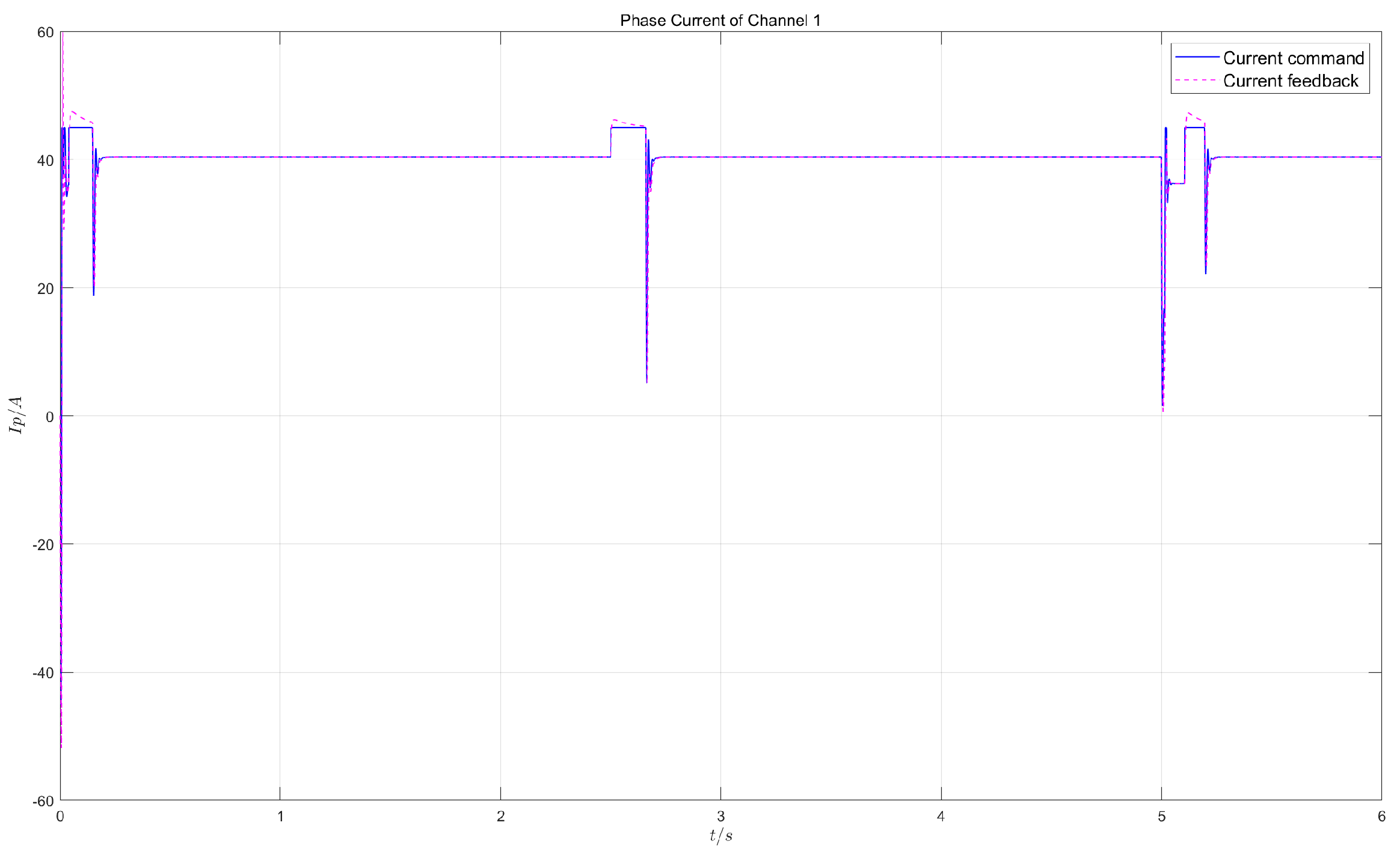
Comparing the results of Test 1 and Test 2, when the same load is applied, the master-master working mode has a position response time of 0.15s, a response speed reaching 8300rpm, and a steady-state current of 20A. The master-standby working mode has a position response time of 0.19s, a maximum response speed of 7900rpm, and a steady-state current of 40A. In terms of response speed, motor heating, etc., the master-master working mode has obvious advantages over the master-standby working mode.
6. Conclusion
Aiming at the requirements of high reliability, high dynamic response, and high-precision control for advanced aircraft actuation systems, this paper realizes the master-master working mode control technology for dual-redundancy EHA systems. The current loop decoupling technology based on vector control is designed, and the robustness of the speed loop and the disturbance rejection capability of the position loop are improved by combining ASMC and improved ADRC. A two-level collaborative control strategy of "position synchronization-current balancing" based on the CCC strategy is proposed to solve the problems of synchronization error accumulation and load imbalance in the master-master mode. Experimental results show that the position loop control error is below ±0.02mm, and the load distribution accuracy is improved to more than , meeting the design requirements of advanced aircraft. The research results of this paper provide important technical support for the engineering application of power-by-wire flight control systems in advanced aircraft.
Author Contributions
Conceptualization, Y.L., X.B. and R.W.; methodology, X.B. and Z.W.; software, X.B.; validation, Z.W. and R.W.; formal analysis, X.B.; investigation, Y.L. and R.W.; resources, Y.L. and X.B.; data curation, Y.L.; writing—original draft preparation, X.B.; writing—review and editing, Y.L. and R.W.; visualization, X.B.; supervision, Z.W.; project administration, Y.L. All authors have read and agreed to the published version of the manuscript.
Funding
This research received no external funding.
Data Availability Statement
The data presented in this study are available on request from the corresponding author. The data are not publicly available due to privacy.
Conflicts of Interest
The authors declare no conflicts of interest.
References
- Ke, Y. , Li, Y., Cao,Y., Zhang,X. Research on model-based safety analysis of flight control system. System Engineering and Electronics 2021, 43, 3259–3265. [Google Scholar]
- Xing, X. , Luo, Y., Han, B., Qin, L., Xiao, B. Hybrid Data-Driven and Multisequence Feature Fusion Fault Diagnosis Method for Electro-Hydrostatic Actuators of Transport Airplane. IEEE Transactions on Industrial Informatics 2025, 21, 3306–3315. [Google Scholar] [CrossRef]
- Bae, J. A Review of Electric Actuation and Flight Control System for More/All Electric Aircraft. 24th International Conference on Electrical Machines and Systems (ICEMS) 2021, 1943–1947. [Google Scholar]
- Robbins, D., Bobalik, J.,Stena, D., Plag, K., Rail, K., Wal, K. F-35 Subsystems Design, Development, and Verification. Aviation Technology, Integration, and Operations Conference 2018, 365-398.
- Wiegand, C. F-35 Air Vehicle Technology Overview. Aviation Technology, Integration, and Operations Conference.
- Guan, L. , Lian, W. Review on Electro-Hydrostatic Actuation Technology of Aircraft Flight Control Actuation System. Measurement & Control Technology 2022, 41, 1–11. [Google Scholar]
- Tai, M. , Yu, H., Zhao, Z., Liu, Z., Zhu, Y. Research on Control of Double-pump Electro-Hydrostatic Actuator ( EHA). Aircraft Design 2023, 43, 31–35. [Google Scholar]
- Yang, X. , Wang, X., Wang, S., Puig, V. Switching-based adaptive fault-tolerant control for uncertain nonlinear systems against actuator and sensor faults. Journal of the Franklin Institute 2023, 360, 11462–11488. [Google Scholar] [CrossRef]
- Dills, P. , Dawson-Elli, A., Gruben, K., Adamczyk, P., Zinn, M. An Investigation of a Balanced Hybrid Active-Passive Actuator for Physical Human-Robot Interaction. IEEE Robotics and Automation Letters 2021, 6, 5849–5856. [Google Scholar] [CrossRef]
- Fu, J. , Maré, J., Fu, Y. Modelling and simulation of flight control electromechanical actuators with special focus on model architecting, multidisciplinary effects and power flows. Chinese Journal of Aeronautics 2017, 30, 47–65. [Google Scholar] [CrossRef]
- Huang, L. , Yu, T., Jiao, Z., Li, Y. Research on Power Matching and Energy Optimal Control of Active Load-Sensitive Electro-Hydrostatic Actuator. IEEE Access 2021, 9, 51121–51133. [Google Scholar] [CrossRef]
- Ahn, K. , Nam, D., Jin, M. Adaptive Backstepping Control of an Electrohydraulic Actuator. IEEE/ASME Transactions on Mechatronics 2014, 19, 987–995. [Google Scholar] [CrossRef]
- Bai, L. , Cui, N., He, M., Zhang, Y. Research on Electro-hydrostatic Actuator(EHA) Load Matching Method. Hydraulics Pneumatics & Seals 2022, 4, 59–65. [Google Scholar]
- Qiu, Y. , Li, Y., Liu, Y., Wang, Z., Liu, K. Observer-based robust optimal control for helicopter with uncertainties and disturbances. Asian Journal of Control 2023, 25, 3920–3932. [Google Scholar] [CrossRef]
- Sui, H. , Liu, W., Zhou, H. Design of servo control system based on fuzzy adaptive PI. Journal of the Hebei Academy of Sciences 2024, 41, 49–54. [Google Scholar]
- Lin, Y. , Shi, Y., Burton, R. Modeling and Robust Discrete-Time Sliding-Mode Control Design for a Fluid Power Electrohydraulic Actuator (EHA) System. IEEE/ASME Transactions on Mechatronics 2013, 18, 1–10. [Google Scholar] [CrossRef]
- Ali, S. , Christen, A. and Begg, S., Langlois, N. Continuous–Discrete Time-Observer Design for State and Disturbance Estimation of Electro-Hydraulic Actuator Systems. IEEE Transactions on Industrial Electronics 2016, 63, 4314–4324. [Google Scholar] [CrossRef]
- Li, Z. , Zhang, Q., An, J., Liu, H., Sun, H. Cross-coupling control method of the two-axis linear motor based on second-order terminal sliding mode. J Mech Sci Technol 2022, 7, 1485–1495. [Google Scholar] [CrossRef]
- Fan, D. , Liu, H., Su, Y. Integral robust collaborative control of hydraulic servo system based on cross-coupling. IEEE Transactions on Industrial Electronics 2025, 53, 81–87. [Google Scholar]
- Yao, J. , Cao, X., Zhang, Y., Li, Y. Cross-coupled fuzzy PID control combined with full decoupling compensation method for double cylinder servo control system. J Mech Sci Technol 2018, 32, 2261–2271. [Google Scholar] [CrossRef]
- Qi, H. , Teng, Y. Force equalization control for dual-redundancy electrol-hydrostatic actuator. Journal of Beijing University of Aeronautics and Astronautics 2017, 43, 270–276. [Google Scholar]
- Zhou, F. , Liu, H., Zhang, P., Ouyang, X. Xu, L., Ge, Y., Yao, Y., Yang, H. High-Precision Control Solution for Asymmetrical Electro-Hydrostatic Actuators Based on the Three-Port Pump and Disturbance Observers. IEEE/ASME Transactions on Mechatronics 2023, 28, 396–406. [Google Scholar] [CrossRef]
- Hong, H. , Gao, B., Li, J. Sliding Mode-PID Control for Aircraft Electro-Hydrostatic Actuator. Civil Aircraft Design & Research 2023, 131, 42–46. [Google Scholar]
Figure 1.
EHA architecture diagram.
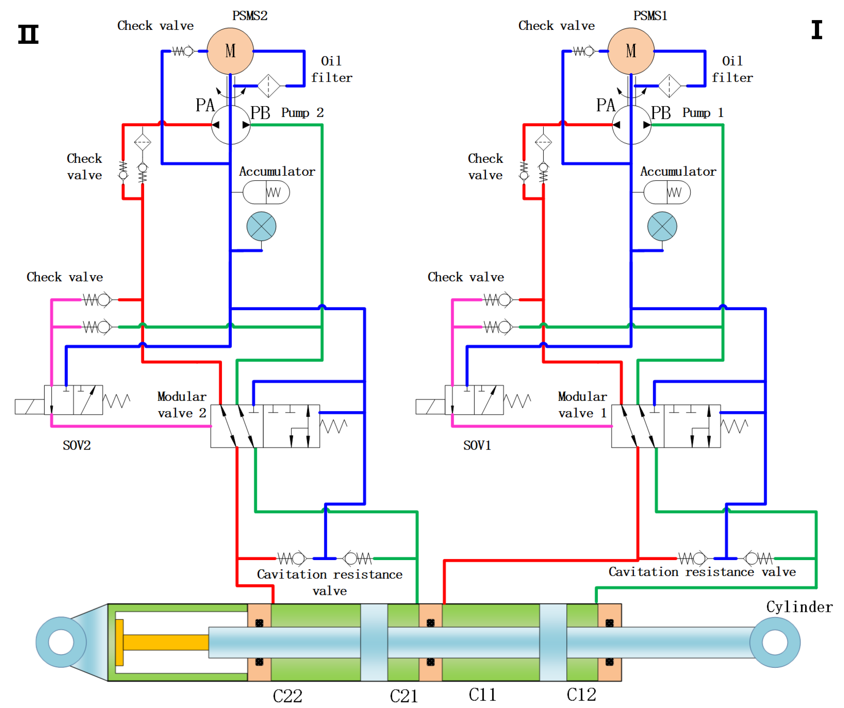
Figure 2.
Actuator controller architecture diagram.
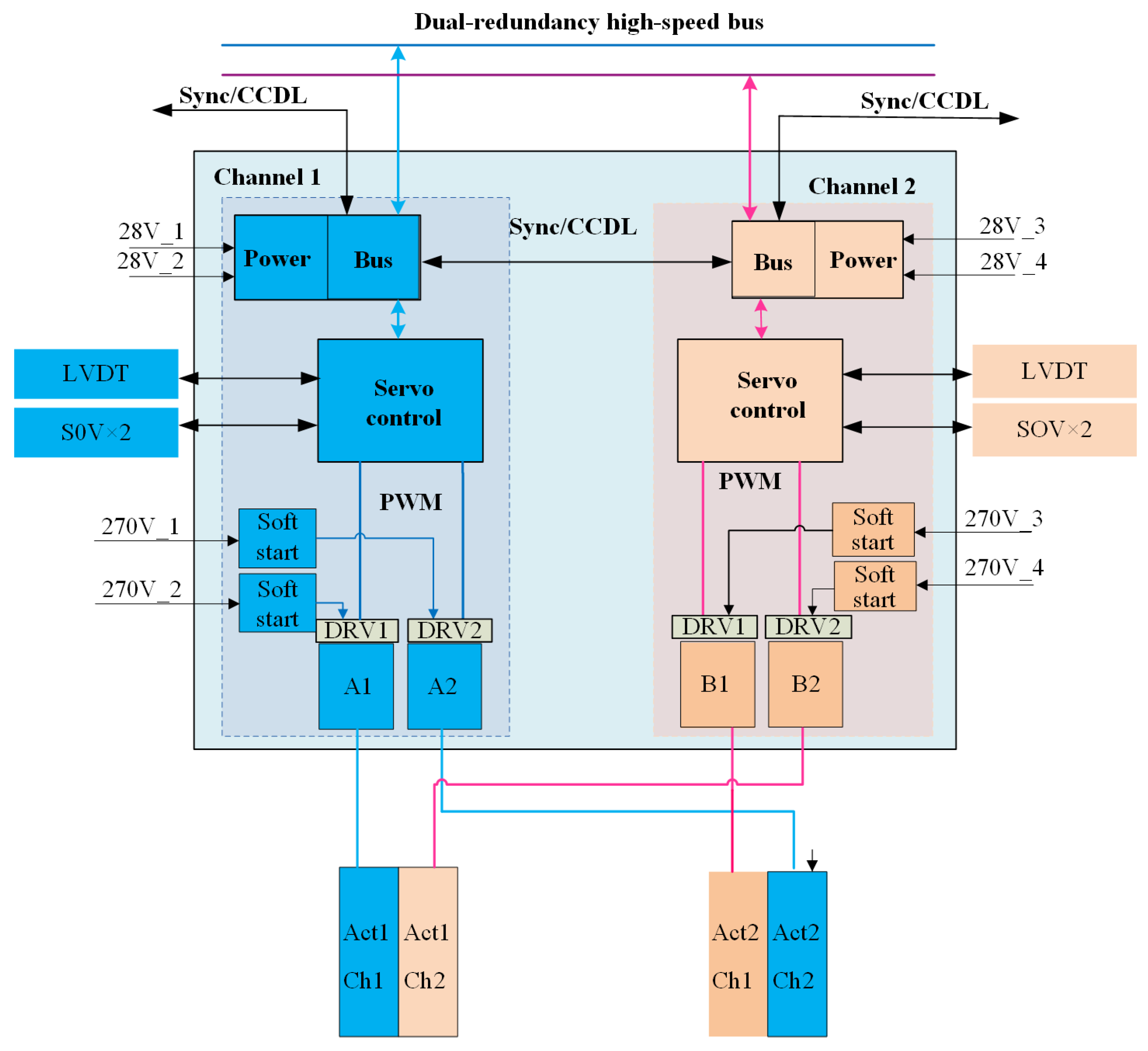
Figure 3.
Position control effect in dual-redundancy master-master working mode.
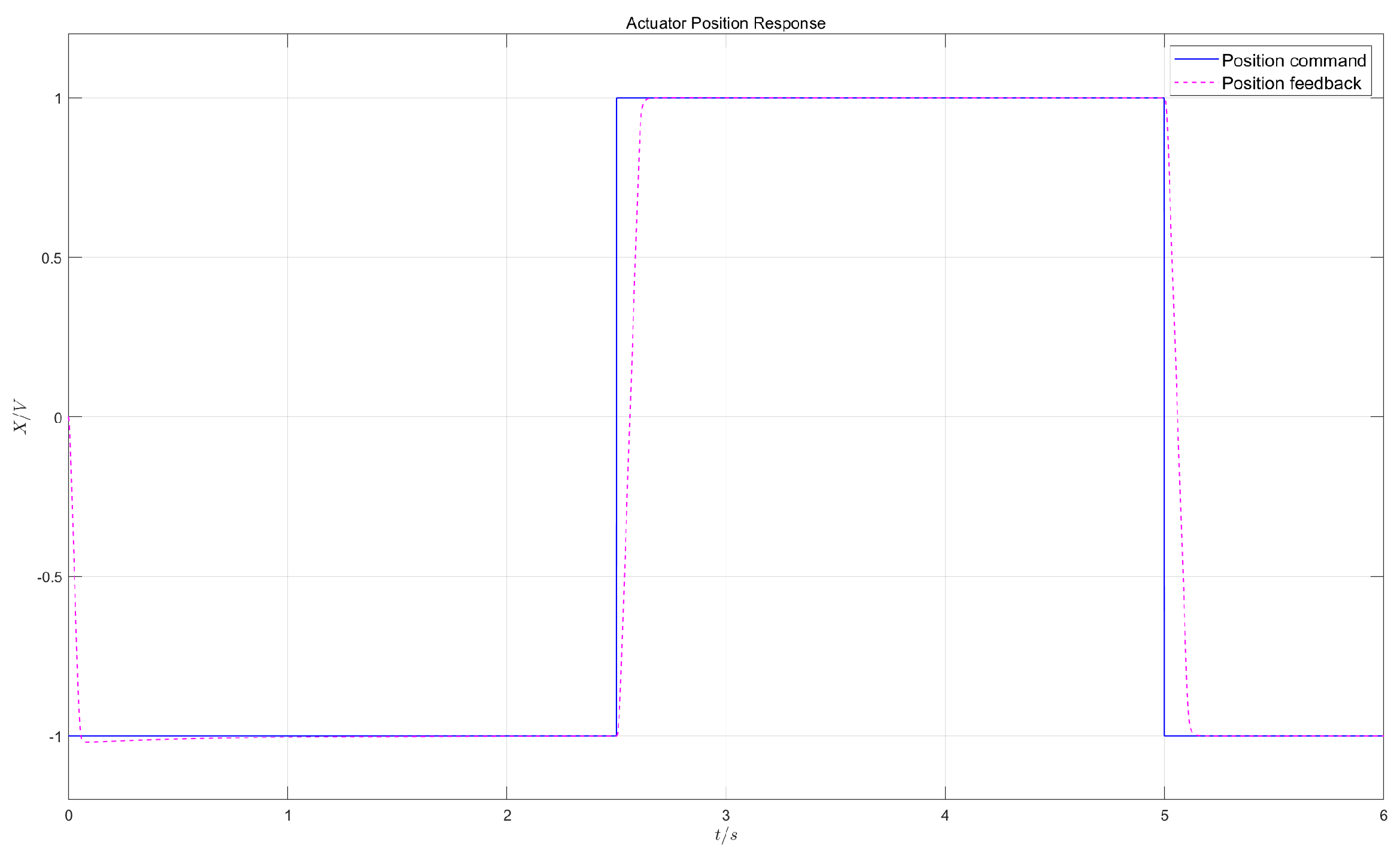
Figure 4.
Motor speed control effect in dual-redundancy master-master working mode.
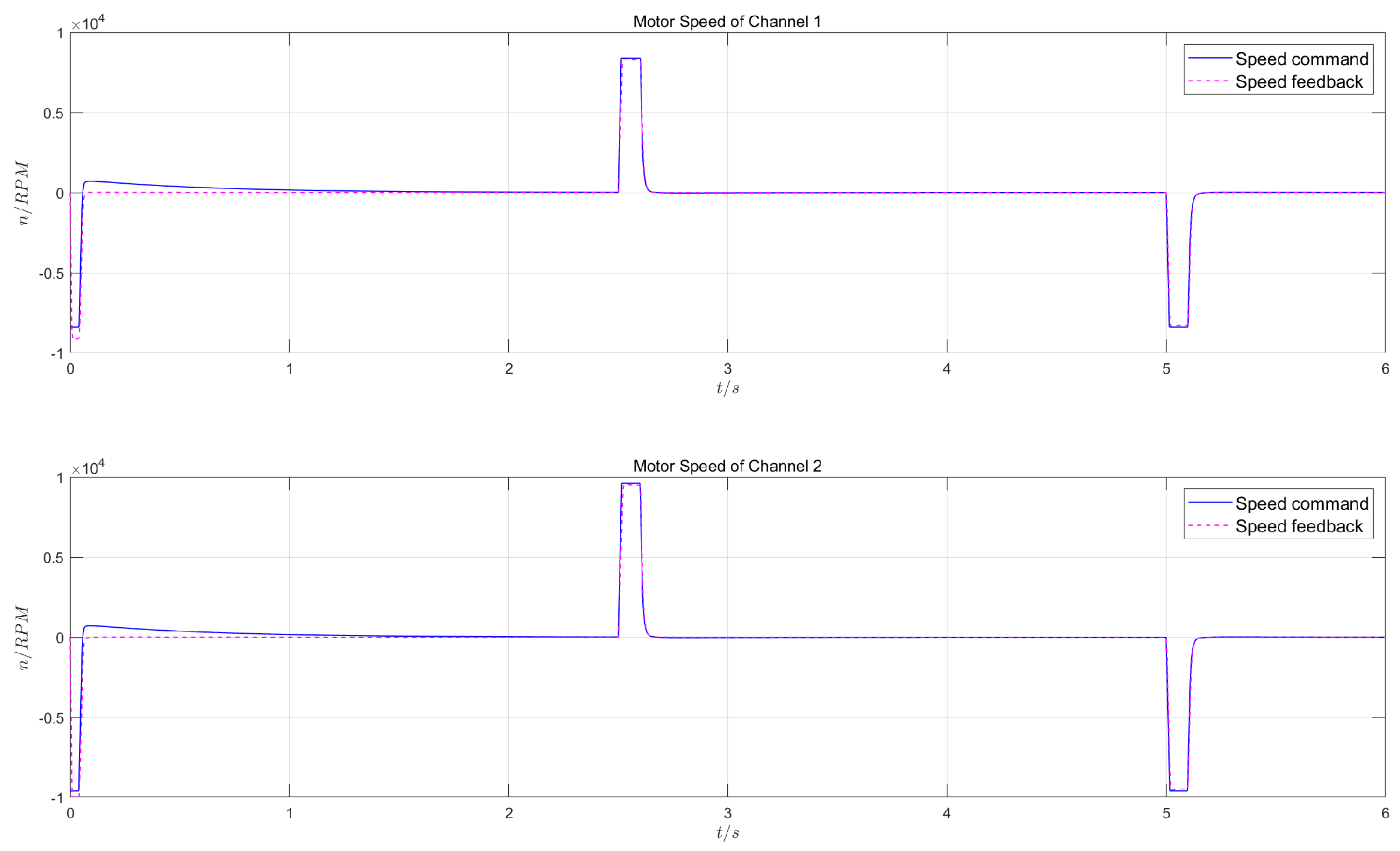
Figure 5.
Motor phase current control effect in dual-redundancy master-master working mode.
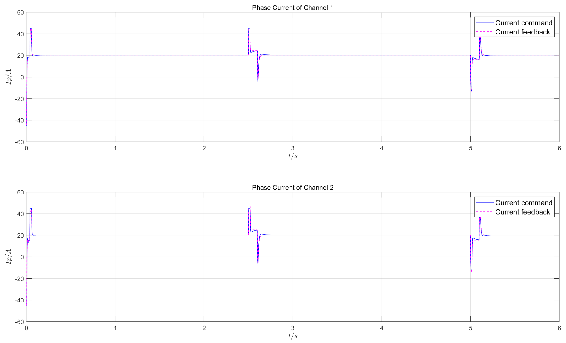
Figure 6.
Position control effect in dual-redundancy master-standby working mode.
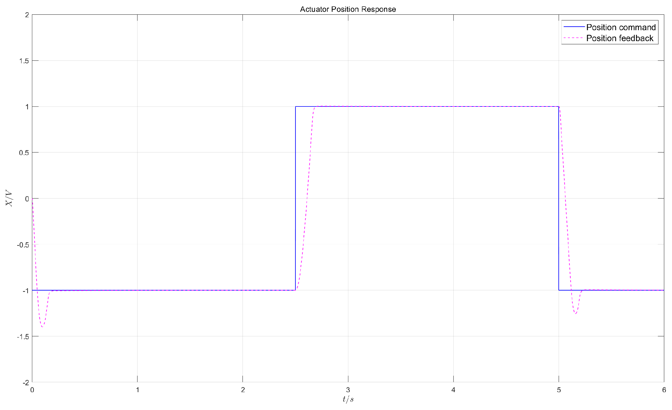
Figure 7.
Motor speed control effect in dual-redundancy master-standby working mode.
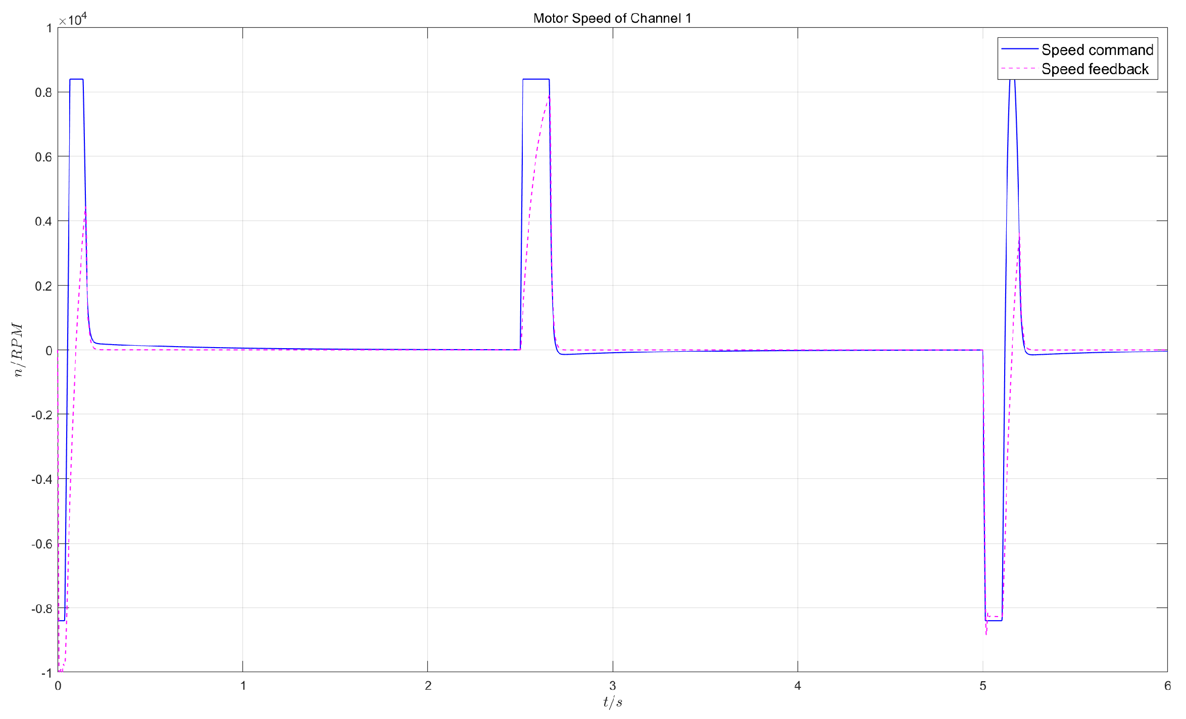
Figure 8.
Motor phase current control effect in dual-redundancy master-standby working mode.
Disclaimer/Publisher’s Note: The statements, opinions and data contained in all publications are solely those of the individual author(s) and contributor(s) and not of MDPI and/or the editor(s). MDPI and/or the editor(s) disclaim responsibility for any injury to people or property resulting from any ideas, methods, instructions or products referred to in the content. |
© 2025 by the authors. Licensee MDPI, Basel, Switzerland. This article is an open access article distributed under the terms and conditions of the Creative Commons Attribution (CC BY) license (http://creativecommons.org/licenses/by/4.0/).
Copyright: This open access article is published under a Creative Commons CC BY 4.0 license, which permit the free download, distribution, and reuse, provided that the author and preprint are cited in any reuse.


