
Submitted:
04 June 2025
Posted:
11 June 2025
You are already at the latest version
Abstract
The double wishbone suspension (DWS) system is widely used in automotive engineering because of its favorable kinematic properties which affect vehicle dynamics, handling, and ride comfort; hence, it is important to have an accurate 3D model, simulation, and analysis of the system in order to optimize its design which requires efficient computational tools for parametric study. The development of effective computational tools which support parametric exploration stands as an essential requirement. Our research demonstrates a complete Wolfram Mathematica system which creates parametric 3D kinematic models and conducts simulations and analyses and generates interactive visualizations of DWS systems. The system uses homogeneous transformation matrices to establish the spatial relationships between components relative to a global coordinate system. The symbolic geometric parameters allow designers to perform flexible design exploration and the kinematic constraints create an algebraic equation system. The numerical solution function NSolve computes linkage positions from input data which enables fast evaluation of different design parameters. The integrated 3D visualization module based on Mathematica′s manipulate function enables users to see immediate results of geometric configurations and parameter effects while calculating exact 3D coordinates. The resulting robust, systematic, and flexible computational environment integrates parametric 3D design, kinematic simulation, analysis, and dynamic visualization for DWS, serving as a valuable and efficient tool for engineers during the design, development, assessment, and optimization phases of these complex automotive systems.
Keywords:
double wishbone suspension
; Homogeneous transformations
; geometry
; kinematic model
; simulation
; 3D design
1. Introduction
The design and behavior of suspension systems determine how well ground vehicles perform while ensuring safety and delivering comfortable rides [1]. The systems control how vehicle bodies interact with road surfaces, thus affecting vehicle handling dynamics and stability and passenger comfort. The Double Wishbone Suspension (DWS), known as short-long arm (SLA) suspension shown in Figure 1, has become a standard choice for performance and racing vehicles as well as heavy-duty applications [2,3]. Engineers choose this system because its beneficial kinematic properties enable them to adjust camber change and roll center height and scrub radius throughout wheel travel and body roll movements to maximize tire grip and vehicle handling capabilities [4,5].
A DWS system’s kinematic behavior depends on its three-dimensional (3D) geometry, which consists of control arm lengths (wishbones) and their chassis mounting points (hardpoints) and steering linkage geometry [6]. The geometric parameters that differ slightly from standard values produce major changes in wheel orientation and body position, which affects essential performance metrics. The automotive design process requires precise 3D kinematic modeling and simulation tools to evaluate suspension performance, compare design alternatives, and optimize geometry before physical prototyping becomes necessary [7].
The optimization of DWS geometry requires examination of a broad design space that contains multiple geometric parameters. The analysis demands computational tools that both deliver precise kinematic simulation and enable fast parametric studies [6]. Engineers require tools that enable fast modification of input parameters such as hardpoint coordinates and link lengths while showing the resulting kinematic changes. The designers require effective visualization tools to understand the spatial motion of multiple links in DWS mechanisms because these tools help them identify interference and undesirable kinematic characteristics [9].
Several methods and software tools exist for suspension analysis. High-fidelity simulation capabilities are provided by multibody dynamics (MBD) software packages such as Adams and Simpack, but these tools come with significant costs and difficult learning curves that may restrict their use for rapid design iterations during early development stages or academic research [10,11]. Vector loop and screw theory provide fundamental insights through analytical methods yet become mathematically complex when dealing with complex 3D spatial mechanisms and parametric variations [12]. Programming environments enable flexible custom computational models yet require frameworks that unite accurate mathematical modeling with efficient numerical solutions and user-friendly parametric design features and clear interactive visualization capabilities [13].
The research presents a computational framework in Wolfram Mathematica for parametric 3D kinematic modeling and simulation and interactive visualization of Double Wishbone Suspension systems to meet this need. The framework uses homogeneous transformation matrices for spatial precision and Mathematica’s symbolic and numerical capabilities to create a robust, accessible tool for engineers and researchers. The framework enables engineers to perform parametric geometry definition and automated kinematic constraint equation generation and solution while providing dynamic 3D visualization to efficiently analyze DWS designs.
The rest of this paper is organized as follows: Section 2 presents the mathematical formulation, including the coordinate systems, the use of homogeneous transformations, and the derivation of kinematic constraints. Section 3 explains the implementation of the computational framework in Mathematica. Section 4 shows simulation results and demonstrates the interactive visualization capabilities. Finally, Section 5 provides concluding remarks and suggests directions for future work.
2. Related Work
The double wishbone suspension (DWS) remains an active area of research in automotive engineering because of its favorable kinematic performance and the increasing need for more refined optimization tools. Recent works address a number of complementary challenges, including simplified analytical models, multi-body simulations with flexible components, and integrated methods for geometric optimization and real-time visualization.
The initial approaches depended mainly on basic two-dimensional planar modeling. The rising need for precise wheel alignment parameter predictions of camber, caster, and toe has led researchers to adopt more advanced 3D parametric modeling approaches. The forward kinematics approach employed screw theory to achieve high accuracy, but it had restricted interactive functionality [14]. A matrix-based system to analyze bump-steer effects while emphasizing real-time simulation for motorsport use [6].
A comprehensive 3D multi-body dynamic (MBD) model was created to study the linked suspension effects [3,15]. In [3], authors explained how rubber bush stiffness affects both the static alignment and the transient responses of the system. MBD software tools such as Adams and Simpack deliver powerful functionality, but their use for symbolic or parametric analysis becomes complicated because users need to write complex scripts and perform multiple iterations [16,17].
The field of vehicle suspension geometry research now uses symbolic computation as an alternative solution because it allows designers to embed adjustable parameters for real-time design exploration. In [14] , authors added symbolic expressions of upright orientation to an existing geometric model. A closed-loop system of constraint equations for short–long arm (SLA) suspensions, which they solved algebraically [6]. The research [3,9] , combines formal kinematic constraints with parametric geometry to create reconfigurable suspension prototypes that do not require code rewriting for each new layout.
The advanced computational tools, particularly Wolfram Mathematica, have shown advantages in solving both symbolic and numeric problems [18]. The real-time parameter manipulation through built-in “Manipulate” and symbolic constraint solution within this system creates a more interactive design environment than typical multi-body codes, which operate through scripting [19]. This method reduces the time needed to evaluate camber-toe sensitivity when testing various geometric modifications.
The study in Table 1 demonstrate the capability of symbolic computation for suspension kinematics, but they mainly concentrate on either numerical performance or static geometry exploration. Real-time symbolic geometry solvers with interactive visualization, as presented in this paper, remain rare and underrepresented.
3. Methodology
The section describes a complete symbolic modeling approach to the geometric analysis and visualization of a double wishbone suspension system shown in Figure 2. The method is based on multibody kinematics and uses homogeneous transformation matrices to define the spatial relationships between suspension components. The system is modeled in Wolfram Mathematica, using symbolic computation to derive position vectors, enforce geometric constraints, and solve for unknown joint configurations under varying parameters.
3.1. Coordinate Transformation
3.1.1. Rotation Matrix
The development of three-dimensional models of geometry and kinematics represents the essential base for simulating double wishbone suspension system behavior. The initial step requires establishing spatial relationships and movement capabilities for all suspension assembly components. The spatial transformations of components are made possible by rotation matrices, which operate on the principal axes . The mathematical building blocks known as matrices enable us to model suspension system articulations during wheel travel and steering input and chassis dynamics responses. It establishes rotation operations in symbolic and modular form for modeling purposes.
In 3D mechanics, a rigid body’s orientation can be described by applying successive rotations about coordinate axes. These rotations are typically represented by orthogonal matrices. Here, we define three such matrices:
-
Rotation about the X-axis (pitch)This rotates a point or vector around the X-axis by an angle . It’s used, for instance, to simulate the upper control arm’s pitch motion relative to chassis mounting points.
-
Rotation about the Y-axis (yaw)This rotation is essential to simulate how the wheel steers around a vertical axis, such as when a vehicle turns left or right.
-
Rotation about the Z-axis (roll)This represents rotation about the , often used in modeling chassis roll or wheel tilt caused by lateral forces.
This contains separate functions that take an angle as input to generate rotation matrices. The matrices function as input with coordinate vectors of suspension points or serve as inputs to create compound transformations to simulate complex motions. The matrices serve an essential purpose because they enable the simulation to rotate points on the suspension, like upright pivots, to replicate actual movement. The rotation matrices will serve an essential purpose in our model by determining the position and orientation of moving components, including the upper and lower wishbones and steering knuckle, throughout wheel travel and body roll.
3.1.2. Combine 3D Rotation
Each matrix rotates the coordinate frame around its respective axis, and they are combined in specific orders to reflect the actual mounting orientation of the suspension parts. Multiple axis rotations are combined using matrix multiplication. Two rotation orders are used:
- XYZ Order: Common for the Lower Control Arm and other base-mounted parts.
- ZXY Order: Used for parts like the Upper Control Arm where the rotation hierarchy differs.
These are calculated as:
This step is critical in ensuring the spatial alignment of the components matches the physical reality of how parts are assembled in an actual suspension system. Multiple angular transformations applied in sequence produce their cumulative effect, which the composite rotation functions encapsulate. The double wishbone suspension uses these functions to determine the end spatial orientation of components that experience motions simultaneously during cornering and vertical travel. The ability to use different rotation orders between and provides valuable modeling versatility, which ensures compatibility with various suspension layouts and coordinate systems. The functions establish a basis for exact and flexible dynamic behavior simulation of the suspension assembly.
3.2. Homogeneous Transformation
The ability to rotate components in space needs translation capabilities to move components between different positions. The double wishbone suspension requires this functionality because its control arms and wheel hub need to perform both rotation and 3D translation motions when the suspension compresses or extends. The homogeneous transformation matrix unifies rotation and translation into a single mathematical operation. The formulation provides a unified matrix representation of rigid-body transformation, which includes both orientation and position changes for efficient point transformation calculations and motion chaining between multiple components.
The homogeneous transformation matrix is a matrix that combines a 3D rotation and translation into a single structure. This is critical for transforming points or frames in 3D space in robotics, vehicle kinematics, and mechanical simulation.
rot: a rotation matrix (like rot3D)
trans: a column vector representing translation
The resulting homogeneous transformation matrix is:
We uses ArrayFlatten to assemble this structure by nesting the following submatrices:
- Top-left block: the rotation matrix rot
- Top-right block: the translation vector trans
- Bottom row: a row vector
This matrix allows to perform rigid-body transformations by multiplying it with a homogeneous point vector:
effectively applying both rotation and translation in one step.
The homogeneous transformation matrix provides a unified form to encapsulate both orientation and position, which makes it essential for simulating the complete spatial motion of mechanical components. The double wishbone suspension model employs this matrix to transmit chassis movements that result in wheel hub motion. The system enables exact position and direction calculations following multiple transformations, which supports both visualization and numerical analysis. The model gains the ability to measure geometric results such as camber angle and kingpin inclination and virtual swing arm trajectories through this formulation.
3.2.1. Transformations from Chassis frame to Upper and Lower Control Arm
This step describes how the upper and lower control arms are mounted and oriented relative to the chassis coordinate system with the rotation and transformation frameworks in place. In a real-world double wishbone suspension, these control arms form the foundation of the suspension triangle and dictate the upright’s motion path. We can simulate their relative positions, orientations, and behavior as independent yet connected subsystems by defining transformations from the chassis frame to the UCA and LCA frames. It uses the previously defined composite rotation and homogeneous transformation functions to express this relationship parametrically.
These two functions define rigid-body transformations from the chassis coordinate system to the upper control arm (UCA) and lower control arm (LCA) coordinate systems. Each function takes six inputs: Euler angles(), defining the control arm’s orientation and the translational offsets () defining the control arm’s mounting position on the chassis
- ACUCA[] : This constructs the transformation matrix for the upper control arm using the Z-X-Y (rot3DZXY) rotation sequence. This choice reflects a mounting configuration where roll (Z), camber/caster tilt (X), and toe or fore-aft direction (Y) are sequentially applied — often relevant to higher control arms whose mounts might be angled or non-orthogonal to the main chassis frame. The function returns a matrix representing the full pose (position and orientation) of the UCA frame in the chassis coordinate system.
- ACLCA[] : This defines the lower control arm transformation, using the Z-Y-X (rot3D) rotation sequence. This is a standard Euler sequence for typical orthogonal setups, where the LCA is mounted more parallel to the chassis axes. It likewise returns a homogeneous transformation matrix.
In both cases, the translation vector is structured as a column vector:
The result is a homogeneous transformation that can now be used to position and orient suspension elements relative to these control arms — such as link pivot points, the upright, or spring/damper connections.
3.2.2. Transformations from UCA and LCA frames to Upright frame
The control arms now have their positions defined relative to the chassis, so the next step in suspension modeling deals with the upright, which serves as the rigid link between the wheel hub and the upper and lower control arms. The upright’s motion path depends on its connections to control arms and sometimes additional linkages, including tie rods or pushrods. The model uses transformation matrices to describe how the upright relates position-wise and orientation-wise to both the upper and lower control arms. Realistic upright articulation simulation depends on these transformations, which also determine wheel motion simulation. A distinct transformation exists for the connecting rod, which enables the model to represent steering links and load-transmitting members.
- AUCUpright[] : This models the Upper Control Arm to Upright transformation. The transformation employs the Z-X-Y rotation order (rot3DZXY), which works best for systems that rotate first around the Z-axis, then translate along the X-axis, and finally rotate around the Y-axis. The matrix is composed with a translation vector , which specifies the physical mounting position of the upright relative to the UCA.
- ALCUpright[] : This transformation connects the Lower Control Arm to the Upright. It follows the Z-Y-X Euler sequence (rot3D), which is suitable for most mounting configurations where the upright moves vertically with LCA travel while also rotating due to steering input.
- ACRod[] : This transformation defines a rod or link, likely used as a tie rod or pushrod. The rotation is limited to the Y and Z axes, as given by rot3D[0, , ], indicating that the rod pivots only in yaw and roll directions. This reflects typical tie rod behavior—steering left and right while allowing vertical compliance. Again, the translation vector defines the position of this rod base relative to the chassis frame or another reference component.
This model defines transformation matrices from control arms and connecting rods to the upright to establish a clear modular pathway for simulating upright behavior under suspension articulation. These functions encode both the geometry and orientation of the links, ensuring that the upright responds correctly to control arm movement and steering input. The separate rod transformation enables steering dynamics or force transmission through tie rods or actuators. The collective transformations create a fully constrained spatial framework for the upright which enables realistic wheel movement and suspension kinematics and structural and dynamic system interactions.
3.3. Local Frame Point
Any multibody mechanical system requires defining essential geometric points that represent mounting and connection interfaces between components, especially in spatial mechanisms such as the double wishbone suspension. The system includes inboard and outboard pivots of control arms together with upright connection points and link attachment points for rods and dampers. The points exist initially within their specific component local coordinate frames. The points become compatible with transformation matrices through homogeneous coordinates (with a fourth coordinate of 1) for accurate mapping between the global (chassis) frame and intermediate frames. The following code establishes such points parametrically to enable complete suspension kinematic assembly.
Homogeneous points — vectors in 4D of the form:
The transformation matrices we built before become directly compatible with the homogeneous points .
- Upper Control Arm (UCA) : pUCAinF[] is the inboard (frame) mounting point of the UCA — typically attached to the chassis. pUCAinR[yUCAinR] is a parameterized inboard mounting on a rail, offset in the Y-axis. The parameter allows users to model various mount points. pUCAout[xUCAout, yUCAout] is the he outer (upright) connection point of the UCA in its local frame.
- Tie Rod or Pushrod : pRodin[]: The base point of the rod in its frame (likely attached to the steering rack or chassis). pRodout[xRodout]: The upright-end attachment point of the rod, parameterized by X — commonly used in steering simulations.
- Upright : pUprightU[xUprightU] is the upper pivot point where the UCA connects to the upright. pUprightL[] is the lower pivot point of the upright, often aligned as the origin in its local frame. pUprightS[xUprightS, yUprightS] is a side point on the upright — likely for the tie rod or shock mount.
- Lower Control Arm (LCA) : pLCAinF[] is the inboard (frame) mounting of the LCA. pLCAinR[yLCAinR] is another inboard option along the Y-axis. pLCAout[xLCAout, yLCAout] is the outer joint where the LCA connects to the upright.
These points operate as plug-and-play components because we specify the configuration through parameters (like xUCAout or yLCAinR) before applying transformation matrices to obtain the global position of each point. The kinematic simulation depends on this fundamental structure.
The point definitions create the geometric structure of the double wishbone suspension model. The model becomes structured and scalable for computing global positions through transformation matrices by describing connection points within their respective local frames using homogeneous coordinates. The system logic remains intact because the overall structure functions independently of link, arm or upright repositioning or reorientation. Engineers can perform geometric changes through this point parametric definition to test different mounting positions and lengths and angles for performance tuning and packaging analysis.
3.4. Global Transformation
After defining geometric points in their local component frames, it becomes necessary to express their positions relative to a global reference frame, typically the chassis or world coordinate system. This transformation is crucial for visualizing the complete suspension layout and for performing kinematic analysis, such as measuring wheel travel paths, camber change, and linkage motion. We can map those points into the global frame by applying the previously defined homogeneous transformation matrices to each local point. This step allows us to track how each suspension component moves in space in response to changes in input parameters such as control arm angles, mount positions, or suspension articulation.
3.4.1. Global Transformation of UCA Points
The Dot operator in Wolfram Language performs matrix multiplication between a transformation matrix and a local point to compute global (chassis-relative) coordinates of key points on the Upper Control Arm (UCA) for each of these functions.
- pUCAinFglobal[...] computes the global coordinates of the UCA’s inboard frame mount, i.e., where the UCA attaches to the chassis. ACUCA[...] is the transformation from the chassis frame to the UCA frame. pUCAinF[] is the local point . Their matrix product yields the global position of the UCA’s inboard frame point.
- pUCAinRglobal[...] is a parameterized inboard point that might slide along a rail (e.g., an adjustable mount position on the chassis). pUCAinR[yUCAinR] introduces a Y-axis offset for the inboard mount. The result gives the real-time global position based on chassis parameters and input angle.
- pUCAoutglobal[...] gives the global coordinates of the UCA’s outboard end, where it connects to the upright. The point pUCAout[xUCAout, yUCAout] defines this connection in local frame coordinates. After applying the chassis → UCA transformation, the returned position can be used to define the upright’s upper ball joint position, measure kinematic variables like camber change or virtual swing arm length, and to visualize the actual suspension arm position in space.
The spatial modeling process reaches its conclusion through these functions, which transform local component geometry into a single global frame. The model uses previously developed transformation matrices to determine the precise positions of critical suspension points throughout three-dimensional space. The model enables both visual inspection and precise calculation of suspension motion through wheel path simulation and instantaneous center tracking and interference checking. The globally transformed points enable the measurement of alignment angles and definition of linkage constraints as well as suspension system integration into complete vehicle dynamics simulations. The transformation step functions as a vital connection between theoretical geometry and actual motion.
3.4.2. Global Transformation of LCA Points
After converting the upper control arm points to the global frame, we need to perform the same operation for the lower control arm (LCA) because it determines the suspension roll center and camber motion behavior. The LCA’s local frame establishes its geometric properties, but its global transformation reveals how it attaches to and moves relative to the chassis reference frame. The transformation enables us to analyze wheel path geometry from the lower link while creating a fully constrained model when combined with the upper link and upright.
- pLCAinFglobal[...] calculation determines the global (chassis-relative) location of the lower control arm’s (LCA) inboard mount, which serves as the chassis-side pivot point. The transformation applies the origin point of the LCA frame through the LCA-to-chassis transformation matrix.
- pLCAinRglobal[...] is a parameterized inboard mount located along the Y-axis, offset from the LCA’s local origin. The parameter allows users to model different LCA pivot positions, which is useful for creating adjustable or performance-optimized suspension geometries.
- pLCAoutglobal[...] defines the outer pivot point of the LCA in global space. The simulation becomes easier to modify using the inputs and , which control the LCA’s length and orientation in space. The actual spatial position of the lower ball joint becomes available through this function, enabling upright motion analysis, camber studies, and suspension force line calculations.
These LCA global point work similarly to the UCA functions and are essential for building the wishbone suspension triangle. This enables intersection point analysis, motion simulation, and force resolution as the model is extended.
3.4.3. Global Transformation of Rod Points
The suspension system contains control arms together with tie rods pushrods and steering arms as supplementary linkages. These components serve to transfer forces while guiding motion between the chassis and upright structure. The complete integration of these components into the 3D suspension model requires transforming their geometric points from local frames into the global coordinate system. The calculation of rod-like component positions in the global coordinate system follows the same homogeneous transformation approach which was used for control arms. The rod achieves precise spatial integration through this method which enables dynamic simulation or visual representation of its interaction with other suspension components.
- pRodinglobal[...] is the base of the rod undergoes transformation into the global frame during this operation. The point pRodin[] has coordinates in the local coordinate system of the rod. The transformation matrix performs spatial orientation through yaw () and roll (), and applies a spatial offset to describe the rod’s positioning and angular orientation in space.
- pRodoutglobal[...] explain the calculation of this endpoint represents the outer end of the rod, which could potentially connect to the upright. The input specifies the extent and orientation of the rod in its local coordinate system along the X-axis. The output provides the actual global coordinates of this endpoint, enabling calculations for steering angle effects, tie rod length changes during articulation, and contact point tracking with the upright.
The rod behaves kinematically like other suspension components because these transformations define it fully in 3D space for dynamic simulation. The functions determine the final spatial arrangement of the rod linkage by translating local coordinates to global coordinates. The transformation step models a steering tie rod and a pushrod in a rocker-arm suspension so the rod can interact meaningfully with other suspension components. The established position enables the restriction of upright motion and wheel alignment guidance during loaded conditions as well as the assessment of link length modifications from steering and bump movements.
3.4.4. Transformations Chaining to Global Upright
The upright serves as a link between the upper and lower control arms to determine wheel orientation. The upright position requires derivation through control arm geometry because it does not attach directly to the chassis. The function creates two transformation matrices which represent the relationship between the chassis and lower control arm (LCA) and between the LCA and upright. The chained transformation enables complete upright pose calculation in the global chassis frame, which enables tracking of suspension motion for wheel and steering geometry transformation.
The function ACUpright is defined as a composition of two transformation matrices:
ACUpright[...] function generates a homogeneous transformation matrix that defines the relationship between the upright’s local frame and the chassis frame through its connection with the Lower Control Arm (LCA). ACLCA(0, , 0, 0, 0, 0) represents the transformation from the chassis to the LCA. The Y-axis rotation angle remains active in this transformation, which may symbolize body roll, wheel travel, or control arm swing. The translation values are zero, indicating that the pivot point of the LCA is fixed in the chassis coordinate system. (ALCUpright()) represents the transformation from the LCA to the upright. It includes a full Euler rotation defined by the angles , and a translation in the LCA frame by , which positions the upright base. The order of transformations is important and it first transforms from the upright to the LCA, then from the LCA to the chassis.
4. Constraint
The mathematical simulation of the constraint requires deriving equations that match the global coordinates of the connection. The vector equations enforce rigid connections between components, and their solutions provide the necessary parameters. The established equations enable future calculations of unknown geometric or motion parameters, including joint positions and angles and translations across various kinematic configurations.
4.1. Upright Constraint Equations
We form the equations that constrain the upper connection point of the upright (like the upper ball joint) to the end of the upper control arm (UCA). This essentially creates a kinematic constraint, a mathematical expression of the mechanical linkage, and is crucial for solving the positions of unknowns in the simulation.
It evaluates two 4D homogeneous coordinate vectors which represent the upright upper point and the UCA outboard point. The function Thread[...] generates three scalar equations by comparing the first three elements of these vectors (excluding the homogeneous coordinate 1), thus establishing spatial dimension constraints for a physical connection.
- leftHandSideU : The global position of the upper joint on the upright is defined by this expression. The computation uses pUprightUglobal[...] which internally applies the transformation ACUpright[...] to the local point pUprightU[]. The inputs specify the upright’s orientation and translation through its linkage connection to the LCA.
- rightHandSideU : The global position of the outboard end of the UCA is represented by this expression. The transformation of a local point through the UCA’s chassis-relative transformation is computed by pUCAoutglobal[...]. This result represents the expected global position where the UCA connects to the upright.
-
equationsU = Thread[...] : The Thread function applies element-wise equality to create:This results in three scalar equations: one for the X-coordinate match, one for the Y-coordinate match, and one for the Z-coordinate match.
These equations impose a rigid body constraint by forcing the UCA outboard point to coincide with the upright upper attachment point in 3D space. The geometric condition is satisfied when these equations are solved, resulting in specific values for unknowns such as link orientations or translation parameters. The constraint equations serve to maintain the rigid link between the upper control arm and upright in the suspension model. These nonlinear vector equations form a system that maintains spatial consistency between interconnected components. The model uses these equations to determine unknown parameters such as joint positions, link lengths or rotational angles during suspension articulation. The technique converts the geometric configuration into a solvable kinematic system which serves as the foundation for numerical simulation, parametric analysis or optimization of suspension behavior. These equations serve as the basis for both validating and dynamically solving the suspension’s motion.
4.2. Constraint Equation for Upright–Rod Connection
The upright component in various suspension systems features an attachment point on its side which accepts auxiliary links including tie rods or pushrods. The rods function to guide steering or transmit loads while requiring kinematic connection to the upright throughout motion. The simulation requires vector equations that establish an exact relationship between the rod’s outboard end position and its attachment point on the upright. The equations guarantee that the upright and rod maintain their rigid connection throughout articulation, which is essential for precise suspension or steering modeling.
- leftHandSideS : It determines the absolute (global) coordinates of a specific upright point that typically hosts rod connections. The local point pUprightS is defined within the upright’s local coordinate system at coordinates and . The transformation ACUpright is applied in the function pUprightSglobal to convert points from the upright’s frame to the global frame. This point dynamically tracks upright movement, as the upright adjusts its position based on Lower Control Arm (LCA) motion and orientation.
- rightHandSideS : This represents the rod’s outboard end, the point that links to the upright. The function pRodout(x_Rodout) determines the endpoint’s coordinates in the rod’s local reference system. The transformation pRodoutglobal applies rod-specific rotation and translation data relative to the chassis, converting the local coordinates into global space. This transformation enables the system to account for steering angle, mounting position, and suspension travel when evaluating the rod’s position.
-
equationsS = Thread[...] : The system generates three individual scalar equations that maintain the spatial relationship between the two global points :This constraint ensures that the upright side point precisely matches the spatial position of the rod’s outboard end.
5. Visualization Framework
The next step after creating a complete kinematic model of the double wishbone suspension in homogeneous coordinates is to obtain the 3D positions for visualization as shows in Figure 3. In a homogeneous system, all spatial points are represented as 4D vectors of the form [x,y,z,1], which allow for matrix multiplication with transformation matrices. However, for graphical rendering or spatial plotting, we only need the 3D position [x,y,z]. The following functions convert transformed homogeneous points to 3D coordinates by removing the fourth component, enabling the construction of lines, linkages, and 3D models of the suspension system.
5.1. Position Points for Visualization
Each function below extracts a 3-element list from a transformed 4-element point using the Most function, which drops the final element (which is always 1 in homogeneous coordinates):
-
For the Upper Control Arm (UCA) :
- -
- posUCAinF[, , , tx, ty, tz]
- -
- posUCAinR[, , , tx, ty, tz, yUCAinR]
- -
- posUCAout[, , , tx, ty, tz, xUCAout, yUCAout]
These return the 3D positions of:- -
- The inboard fixed and inboard rail-mounted chassis pivots of the UCA
- -
- The outboard end of the UCA, where it connects to the upright
-
For the Lower Control Arm (LCA) :
- -
- posLCAinF[, , , tx, ty, tz]
- -
- posLCAinR[, , , tx, ty, tz, yLCAinR]
- -
- posLCAout[, , , tx, ty, tz, xLCAout, yLCAout]
These return the 3D coordinates of:- -
- Inboard fixed and adjustable LCA pivots
- -
- The upright-side joint on the LCA
-
For the Upright :
- -
- posUprightS[, , , txu, tyu, xUprightS, yUprightS]
- -
- posUprightU[, , , txu, tyu, xUprightU]
These return:- -
- posUprightS: The side attachment point (e.g., tie rod or damper mount)
- -
- posUprightU: The upper attachment point for the UCA
These functions rely on the composite transformation from chassis → LCA → upright. -
For the Rod (Tie Rod or Pushrod) :
- -
- posRodin[, , txr, tyr, tzr]
- -
- posRodout[, , txr, tyr, tzr, xRodout]
These compute:- -
- The rod’s chassis-side mounting (e.g., steering rack connection)
- -
- The rod’s upright-side endpoint
The geometric pipeline reaches its end through these functions, which transform homogeneous suspension points into Cartesian coordinates. The suspension model becomes ready for 3D rendering through Wolfram Language graphics primitives including line, point, and Graphics3D objects. The system becomes capable of animation across different configurations and dynamic response evaluation through this positional definition. These definitions establish the base for visual simulation and technical illustration and interactive analysis of double wishbone suspension geometry.
5.2. Rendering of Suspension System
The visual model functions as a communication tool while providing spatial verification of simulated geometry, and it can be extended to include dynamic animation and design optimization workflows. The figure presents a 3D representation of the double wishbone suspension system in a valid configuration, which results from solving the complete set of kinematic constraints. The positions of all suspension elements are computed using homogeneous transformations and plotted in the chassis coordinate frame.
Graphics3D[{
(* Upper Control Arm *)
Red, Line[{pUCAinFglobalPos, pUCAoutglobalPos}],
Red, Line[{pUCAinRglobalPos, pUCAoutglobalPos}],
Red, Sphere[pUCAinFglobalPos, 0.1],
Red, Sphere[pUCAinRglobalPos, 0.1],
Red, Sphere[pUCAoutglobalPos, 0.1],
(* Lower Control Arm *)
Purple, Line[{pLCAinFglobalPos, pLCAoutglobalPos}],
Purple, Line[{pLCAinRglobalPos, pLCAoutglobalPos}],
Purple, Sphere[pLCAinFglobalPos, 0.1],
Purple, Sphere[pLCAinRglobalPos, 0.1],
Purple, Sphere[pLCAoutglobalPos, 0.1],
(* Upright vertical connection *)
Green, Line[{pUCAoutglobalPos, pLCAoutglobalPos}],
Green, Sphere[pUCAoutglobalPos, 0.1],
Green, Sphere[pLCAoutglobalPos, 0.1],
(* Rod (tie rod / pushrod) *)
Black, Line[{pRodinglobalPos, pRodoutglobalPos}],
Black, Sphere[pRodinglobalPos, 0.1],
Black, Sphere[pRodoutglobalPos, 0.1]\
}
]
In color coding, red indicates the upper control arm, purple represents the lower control arm, green is used for the vertical upright connection, and black corresponds to the rod (such as a steering link or pushrod). The elements with a line[...] denotes mechanical links between components, while sphere[..., 0.1] is used to visualize joints or mounting points in the 3D suspension model.
The visualization function gives a general spatial view of the whole suspension assembly. It provides a clear view of how control arms, the upright and linkages interact in three-dimensional space by color coding the major components and highlighting their joint locations. This visual tool not only aids in verifying model correctness but also supports further enhancements such as dynamic simulation, design optimization, and educational demonstrations. Furthermore, the flexible rendering pipeline allows for real-time updates to suspension geometry and articulation, which enables continuous integration of engineering feedback into the design process.
6. Dynamic Kinematic Solver
The section demonstrates how to model the physical behavior of a double wishbone suspension system under different geometric and alignment conditions by using the Manipulate and NSolve constructs in Wolfram Language to create a dynamic solver. The tool enables users to modify chassis and component parameters in real time while it solves the system of nonlinear equations that maintain mechanical linkage constraints. The visualization automatically updates to show each valid configuration so users can interactively examine different suspension designs and behaviors. Figure 4 shows the results of a dynamic kinematic simulation for the double wishbone suspension model using a constraint-based solver. The system checks whether the upright, control arms, and rod links can meet spatial and mechanical constraints based on user-defined parameters. In successful cases (a and b), the solver produces consistent joint positions that result in a plausible suspension layout, as visually validated by the continuous and symmetric linkage geometry. In cases (c and d), the system is over- or under-constrained, and the solver fails to converge to a valid solution, which resulting in disconnected or distorted linkage representations. This shows the importance of constraint resolution in ensuring physical plausibility within dynamic simulations.
The local scope defines a solution computation and storage area for NSolve together with the unknown joint angles (upper control arm orientation) and (upright orientation through the lower control arm) and (tie rod orientation). The equations define kinematic constraints which show the positions that must match in 3D space for parts to be physically connected. The equationsU expression verifies that the upper point of the upright corresponds to the UCA outboard joint and the equationsS expression verifies that the upright side matches the tie rod outboard joint. The system becomes solvable through symbolic parameter replacement of manipulated counterparts which leads to a nonlinear system. The system requires domain constraints to prevent unrealistic movements of the upright and tie rod from occurring. The numerical solution of the system yields joint angle values that fulfill every constraint. A valid solution discovered during the process updates the visualization by showing the suspension system with new geometric and angular information to provide immediate feedback for parameter adjustments. The system defaults to a neutral configuration with zero angles when no solution is found to prevent visual display issues. The module includes sliders at its bottom for controlling mount point locations (like xLCAout, txcr, xRodout) as well as initial chassis/UCA orientation (,) and suspension deflection angle (). Users can modify design parameters through sliders to test arm length variations and mounting offset changes while examining how geometry influences suspension performance and feasibility in bump and compression simulations.
The interactive simulation module converts the suspension model into an effective design and analysis instrument. The system enables users to see valid suspension configurations through real-time numerical solving and 3D rendering of symbolic kinematic models. The system proves essential for design engineers who need to evaluate geometry changes, and analyze motion constraints, and detect mechanical infeasibility during early design stages. The module enables real-time exploration of geometry-to-behavior relationships, which makes it essential for the broader modeling framework and a fundamental component for suspension system optimization.
7. Conclusion
This paper presented a novel symbolically driven framework for the 3D geometric modeling, constraint-based solving, and real-time visualization of a double wishbone suspension system framework through symbolic methods. The framework is making a significant contribution by using homogeneous transformations together with Euler-based rotation matrices and symbolic point definitions to construct suspension assemblies precisely and modularly within three-dimensional space. The framework, which combines symbolic kinematic representation with numerical constraint solving and dynamic rendering, establishes a major shift from conventional rigid-body modeling practices because they either fail to provide analytical clarity or real-time interactivity. The framework automatically determines internal degrees of freedom through user-defined geometry by applying nonlinear vector constraints to resolve upright and rod orientations. The system enables real-time visual validation of design choices while maintaining physical feasibility. The model becomes highly accessible through its integration with an interactive manipulation interface, which provides immediate feedback during parameter adjustments and enables engineers and students to explore suspension behavior through intuitive hands-on interaction.
Multiple use cases demonstrated how the framework successfully handled complex suspension configurations while showing their design under different conditions. The system demonstrated both geometric continuity and realistic articulated motion while delivering important insights about design variable impacts on camber and toe kinematic outcomes. The proposed system provides a solid foundation for future research and development activities. The system can be expanded by adding force-based dynamics and optimization routines as well as alternative suspension geometries. The framework provides significant contributions to vehicle dynamics and multibody kinematics and computational design through its use in instructional settings and concept design evaluation and prototype development for advanced simulation platforms.
Author Contributions
Conceptualization, M.W.A.,S.L.; methodology, M.W.A.,S.L.; validation, M.W.A.,S.L.; formal analysis, M.W.A.,S.L.; writing—original draft preparation, M.W.A.; writing—review and editing, S.L. and D.Q.L.; supervision, S.L. and D.Q.L. All authors have read and agreed to the published version of the manuscript.
Funding
Authors disclose support for the research of this work from Ferrari and the European Union under the PNRR (National Recovery and Resilience Plan) under Grant No. 2933.
Data Availability Statement
Not applicable
Acknowledgments
We would like to express our sincere gratitude to the Ferrari Technical Team. T. Davide, F. Alessandro, and F. Rocco for their invaluable support to this research. Their expertise and assistance have been instrumental in completing this work.
Conflicts of Interest
The authors declare no conflicts of interest.
Abbreviations
The following abbreviations are used in this manuscript:
| Symbol | Description | Type / Unit |
| Rotation angle (pitch) of Upper Control Arm (UCA) in chassis frame | Angle (radians) | |
| Rotation angle (yaw) of UCA in chassis frame, solved dynamically | Angle (radians) | |
| Rotation angle (roll) of UCA in chassis frame | Angle (radians) | |
| Rotation angle (pitch) of Upright in LCA frame, solved dynamically | Angle (radians) | |
| Rotation angle (yaw) of Upright in LCA frame, solved dynamically | Angle (radians) | |
| Rotation angle (roll) of Upright in LCA frame, solved dynamically | Angle (radians) | |
| Yaw angle of tie rod (rod) in chassis frame, solved dynamically | Angle (radians) | |
| Roll angle of tie rod (rod) in chassis frame, solved dynamically | Angle (radians) | |
| Suspension bump angle / deflection used to drive motion (applies to LCA) | Angle (radians) | |
| X-coordinate of the UCA outboard connection in its local frame | Distance (units) | |
| Y-coordinate of the UCA outboard connection in its local frame | Distance (units) | |
| X-coordinate of the LCA outboard connection in its local frame | Distance (units) | |
| Y-coordinate of the LCA outboard connection in its local frame | Distance (units) | |
| X-offset of upright’s upper ball joint in upright local frame | Distance (units) | |
| X-offset of upright’s side connection (tie rod or damper) | Distance (units) | |
| Y-offset of upright’s side connection (tie rod or damper) | Distance (units) | |
| Z-offset of upright’s side connection (if used in 3D placement) | Distance (units) | |
| Y-offset of UCA inboard mount (rail variant) | Distance (units) | |
| Y-offset of LCA inboard mount (rail variant) | Distance (units) | |
| X-translation of UCA frame relative to chassis | Distance (units) | |
| Y-translation of UCA frame relative to chassis | Distance (units) | |
| Z-translation of UCA frame relative to chassis | Distance (units) | |
| X-translation of LCA-to-upright joint in chassis (manipulated input) | Distance (units) | |
| Y-translation of LCA-to-upright joint in chassis | Distance (units) | |
| X-offset of rod mount point in chassis | Distance (units) | |
| Y-offset of rod mount point in chassis | Distance (units) | |
| Z-offset of rod mount point in chassis | Distance (units) | |
| X-length of rod (from inboard to outboard tip) | Distance (units) | |
| pUCAinF[...] | Inboard frame-side point of Upper Control Arm (global) | 3D Position |
| pUCAout[...] | Outboard point of UCA, connects to upright | 3D Position |
| pLCAinF[...] | Inboard chassis-side point of Lower Control Arm (global) | 3D Position |
| pLCAout[...] | Outboard point of LCA, connects to upright | 3D Position |
| pUprightU[...] | Upper upright point where UCA connects | 3D Position |
| pUprightS[...] | Side upright point (tie rod or damper connection) | 3D Position |
| pRodinglobal[...] | Inboard (chassis-mounted) end of rod | 3D Position |
| pRodoutglobal[...] | Outboard (upright-connected) end of rod | 3D Position |
| drawSuspension[...] | Visualization function to render the entire suspension system using all calculated points | Graphics3D |
| solution | Output of NSolve used to extract valid joint angles | List |
| equationsU, equationsS | Constraint equations that ensure connected parts meet at a common point | Equation Set |
| deqs | Merged constraint equations from both UCA and tie rod systems | Equation Set |
| cons | Constraints on angle ranges for physically plausible behavior | Inequality Set |
| NSolve[...] | Numerical solver used to solve nonlinear constraint system | Solver Output |
References
- Dubey, A. D., Verma, S., & Kumar, P. (2022). Analysis of Double Wishbone Suspension System Using MechAnalyzer. In S. Yadav, P. K. Jain, P. K. Kankar, & Y. Shrivastava (Eds.), Advances in Mechanical and Energy Technology (pp. 245–255). Springer, Singapore. [CrossRef]
- Park, H., Langari, R., & Yi, H. (2024). Design and testing of double-wishbone suspension for enhanced outdoor maneuver stability of a six-wheeled mobile robot. Mechatronics, 103, Article 103237. [CrossRef]
- Taneva, S., Ambarev, K., & Penchev, S. (2024). Strength and Frequency Analysis of the Lower Arm of a Double Wishbone Suspension of a Passenger Car. Environment. Technology. Resources. Proceedings of the International Scientific and Practical Conference, 1, 352–357. [CrossRef]
- Sharma, R. (2023). Design and Optimisation of Double Wishbone Suspension for High Performance Vehicles. International Journal of Vehicle Systems Modelling and Testing, 17(2), 185–195. [CrossRef]
- Niu, Z., Jin, S., Wang, R., & Zhang, Y. (2022). Geometry Optimization of a Planar Double Wishbone Suspension Based on Whole-Range Nonlinear Dynamic Model. Proceedings of the Institution of Mechanical Engineers, Part D: Journal of Automobile Engineering, 236(1), 3–14. [CrossRef]
- Avi, A. G., Carboni, A. P., & Stella Costa, P. H. (2021). Multi-objective optimization of the kinematic behaviour in double wishbone suspension systems using genetic algorithm. SAE Technical Paper 2020-36-0154. [CrossRef]
- Shao, Y., Li, G., & Wang, J. (2023). Optimization Design of Double Wishbone Front Suspension Based on Dynamic Simulation. Applied Sciences, 14(5), Article 1812. [CrossRef]
- Arshad, M.W.; Lodi, S.; Liu, D.Q. Multi-Objective Optimization of Independent Automotive Suspension by AI and Quantum Approaches: A Systematic Review. Machines 2025, 13, 204. [CrossRef]
- Upadhyay, P., Deep, M., Dwivedi, A., Agarwal, A., Bansal, P., & Sharma, P. (2020). Design and analysis of double wishbone suspension system. IOP Conference Series: Materials Science and Engineering, 748, 012020. [CrossRef]
- Golightly, D., Pierce, K., Palacin, R., & Gamble, C. (2021). A feasibility assessment of multi-modelling approaches for rail decarbonisation systems simulation. Proceedings of the Institution of Mechanical Engineers, Part F: Journal of Rail and Rapid Transit, 236(2), 115–126. [CrossRef]
- Simpack Multibody Simulation Software. (n.d.). SIMULIA. https://www.3ds.
- Wang, J., & Zhao, Y. (2022). A repelling-screw-based approach for the construction of Jacobian matrices in parallel manipulators. Mechanism and Machine Theory, 170, 104726. [CrossRef]
- Guo, M., De Persis, C., & Tesi, P. (2024). Data-Driven Stabilization of Nonlinear Systems via Taylor’s Expansion. In R. Postoyan, P. Frasca, E. Panteley, & L. Zaccarian (Eds.), Lecture Notes in Control and Information Sciences (pp. 299–315). Springer. [CrossRef]
- Ashtekar, V., & Bandyopadhyay, S. (2021). Forward Dynamics of the Double-Wishbone Suspension Mechanism Using the Embedded Lagrangian Formulation. In D. Sen, S. Mohan, & G. K. Ananthasuresh (Eds.), Mechanism and Machine Science (pp. 843–859). Springer, Singapore. [CrossRef]
- Zhang, B., & Li, Z. (2021). Mathematical modeling and nonlinear analysis of stiffness of double wishbone independent suspension. Journal of Mechanical Science and Technology, 35(12), 5671–5680. [CrossRef]
- Simpack Multibody Simulation Software. (n.d.). SIMULIA. https://www.3ds.com/products/simulia/simpack.
- Adams: The Multibody Dynamics Simulation Solution. (n.d.). Enteknograte. https://enteknograte.com/adams-multibody-dynamics-simulation-solution/.
- Wolfram Research. (n.d.). Symbolic and Numeric Computation. Wolfram U. Retrieved from https://www.wolfram.com/wolfram-u/courses/mathematics/symbolic-numeric-computation-math915/.
- Wolfram Research. (n.d.). Advanced Manipulate Functionality. Wolfram Language Documentation. Retrieved from https://reference.wolfram.com/language/tutorial/AdvancedManipulateFunctionality.
- M. Larcher, D. Stocco, M. Tomasi, and F. Biral. A Symbolic-Numerical Approach to Suspension Kinematics and Compliance Analysis. In: Proceedings of the ASME 2024 International Mechanical Engineering Congress and Exposition. Volume 5: Dynamics, Vibration, and Control, Portland, Oregon, USA, November 17–21, 2024. V005T07A049. ASME. [CrossRef]
- T. Uchida and J. McPhee. Driving Simulator with Double-Wishbone Suspension Using Efficient Block-Triangularized Kinematic Equations. Multibody System Dynamics 28, no. 3 (2012): 331–347. [CrossRef]
- H.-H. Chun and T.-O. Tak. Sensitivity Analysis Using a Symbolic Computation Technique and Optimal Design of Suspension Hard Points. Journal of the Korean Society for Precision Engineering 16, no. 4 (1999): 26–36.
- M. Makita. An Application of Suspension Kinematics for Intermediate Level Vehicle Handling Simulation. JSAE Review 20 (1999): 471–477. [CrossRef]
- K. P. Balike. Kineto-Dynamic Analyses of Vehicle Suspension for Optimal Synthesis. PhD dissertation, Concordia University, 2010.
Figure 1.
Three-dimensional visualization of a double wishbone suspension system detailing the layout of control arms, connection points, and wheel assembly [8].
Figure 1.
Three-dimensional visualization of a double wishbone suspension system detailing the layout of control arms, connection points, and wheel assembly [8].
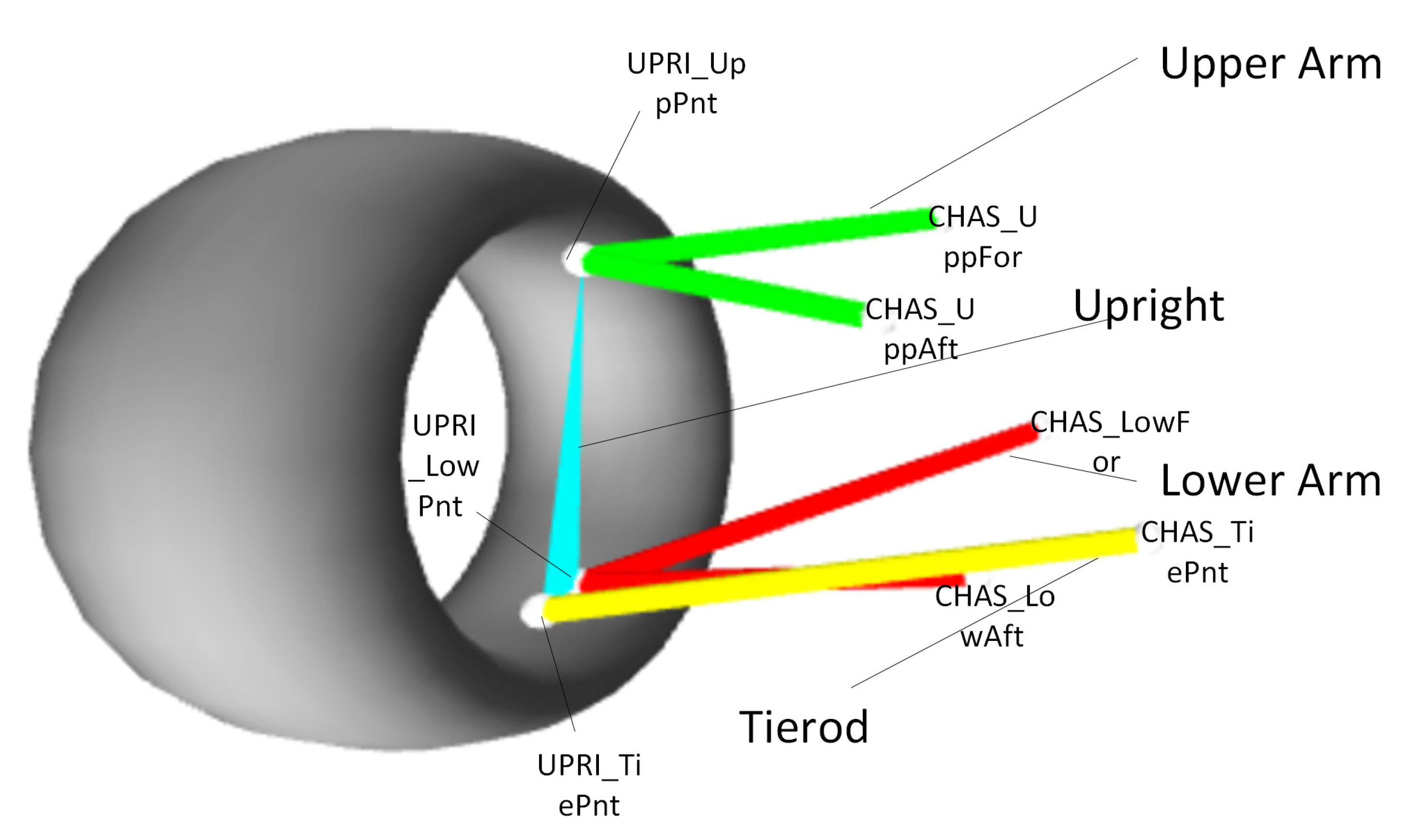
Figure 2.
The schematic diagram illustrates the positional connections between the upper and lower control arms (UCA and LCA), upright, rod linkage and steering input components. The model includes annotated local coordinate axes together with reference points that label each element (like as pUCAout, pUprightS, pRodout). The parameter names xUCAout, yLCAinR and xUprightS represent adjustable geometric values in their respective frames. The diagram shows the component frames (UCA Frame, LCA Frame, Upright Frame) and their transformations and connections through joint locations and linkage endpoints relative to the global reference frame.

Figure 3.
3D geometric visualization of a valid double wishbone suspension configuration. The rendered suspension system shows proper alignment and articulation of the upper and lower control arms (red and purple), the upright (green), and associated links such as tie rods (black). All components are connected and meet geometric and kinematic constraints, which shows a physically consistent assembly under the given parameter set.
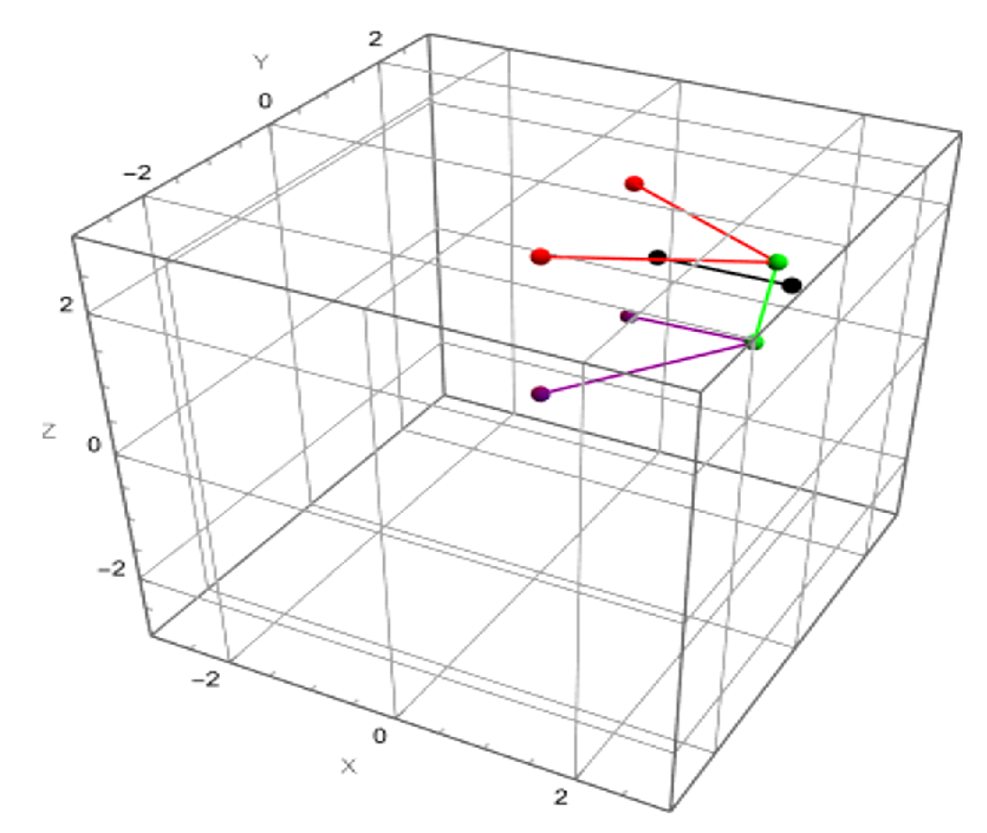
Figure 4.
The kinematic solver successfully identifies valid solutions for all geometric constraints in panels (a) and (b), which produce physically correct component linkage visualizations. The constraint-solving system fails to find valid solutions in panels (c) and (d) because the input parameters lead to visibly incorrect linkage alignment and disconnected joints.
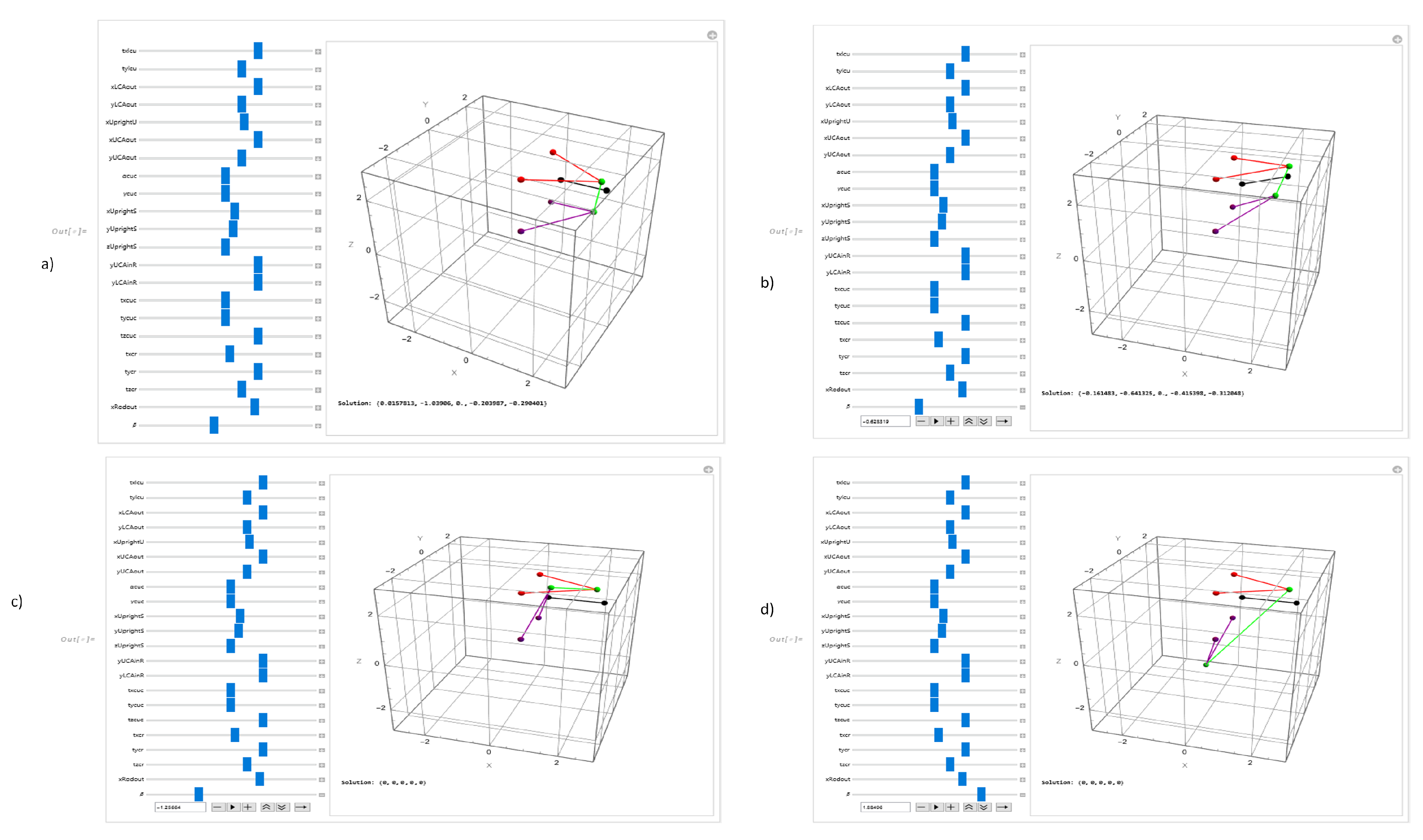

Table 1.
Overview of Symbolic Modeling Approaches for Suspension Systems.
| System Type | Symbolic Method | Focus Area | Visualization | Interactivity |
|---|---|---|---|---|
| General suspensions [20] | Mixed Symbolic-Numerical | K&C modeling | ✗ | ✗ |
| Double wishbone [21] | Block-triangularization | Real-time dynamics | ✓ (simulator) | Partial |
| Generic link suspensions [22] | Symbolic sensitivity analysis | Design optimization | ✗ | ✗ |
| McPherson [23] | Mathematica-based symbolic kinematics | Static geometry | ✗ | ✗ |
| Double wishbone [24] | Coupled kineto-dynamics | Performance trade-offs | ✗ | ✗ |
| Double wishbone | Full symbolic + numerical solving | Real-time kinematics & visualization | ✓ (3D interactive) | ✓ (live parametric solver) |
Disclaimer/Publisher’s Note: The statements, opinions and data contained in all publications are solely those of the individual author(s) and contributor(s) and not of MDPI and/or the editor(s). MDPI and/or the editor(s) disclaim responsibility for any injury to people or property resulting from any ideas, methods, instructions or products referred to in the content. |
© 2025 by the authors. Licensee MDPI, Basel, Switzerland. This article is an open access article distributed under the terms and conditions of the Creative Commons Attribution (CC BY) license (http://creativecommons.org/licenses/by/4.0/).
Copyright: This open access article is published under a Creative Commons CC BY 4.0 license, which permit the free download, distribution, and reuse, provided that the author and preprint are cited in any reuse.


