
Submitted:
10 June 2025
Posted:
10 June 2025
You are already at the latest version
Abstract
Different from the concentrated load, the sliding bearing-wind turbine gearbox coupling interface load is a time-space coupling distributed dynamic load that need to be represented by variables in both temporal and spatial dimensions. In order to apply directly the general shafting transient response method based on concentrated load to analysis transient response of sliding bearing- wind turbine gearbox, a decoupling method for coupling interface load based on POD decomposition algorithm was established to address the spatiotemporal coupling characteristics. In which coupling interface load is decoupled into several sets of space-time independent sub-distributed loads composed of time history and spatial distribution function. The Chebyshev polynomial is used to transformed the spatial distribution function into the concentrated load acting on the limited action point of the shaft system. The improved method is verified by comparing with the results coming from finite element software.
Keywords:
sliding bearing- wind turbine gearbox
; transient response analysis
; distributed dynamic load
; Dop decoupling
; Chebyshev polynomial
1. Introduction
In recent years, “Replacing rolling with sliding” is the future development trend of high-power wind turbine gearboxes. Sliding bearings are the supporting components of high-power wind turbine gearbox transmission systems and are crucial for maintaining stable operation of wind power equipment [1,2]. Bearing capacity and vibration signals are an important indicator for the healthy operation and maintenance of high-power wind power equipment, which is crucial for dynamic design, vibration reduction and isolation design, and reliability analysis. Ding Jiayu proposed an improved linear regression radial basis function neural network method based on principal component analysis. The sliding window residual statistics method is used to monitor the running state of the unit in real time, and the gearbox bearing fault is effectively predicted. Jun Wang [3] used the vibration signals to diagnosis bearing Fault. Pan Qiaobo [5] accurately determines the corresponding position of transient components through the generator displacement vibration information of wind turbine. Su Guoliang [6] and others use the gradient algorithm of integrated machine learning algorithm and the key information of key vibration displacement signals as an important basis for wind turbine generator fault diagnosis. The vibration displacement signals from the transient response analysis under sliding bearing- wind turbine gearbox coupling interface load are the focus of attention.
Different from the rolling bearing, the oil film thickness of the sliding bearing with oil wedge bearing pressure changes with time and space, so that the sliding bearing- wind turbine gearbox coupling interface load is no longer a concentrated dynamic load but a space-time coupling distribution dynamic load. Liu [7] established the oil film load model of rotor-bearing system, and the results show that oil film load is closely related to the change of rotor speed. According to the study of Wang [8], the bearing capacity of oil film varies with position and time. Ling Han [9] obtains the change law of oil film load. Yao Li [10] and others studied the influence of crack coordinate position and rotational speed on sliding bearing. It is known that the oil film load on the wind power gearbox during operation [11] is not only related to the space position, but also related to the running time, showing the characteristics of space dimension and time dimension, which is a kind of space-time coupling distribution load. The vibration displacement response under coupling interface load expressed by variables of time and space dimensions cannot be directly analyzed by Newmark and other concentrated time-domain load transient response analysis method [12,13,14,15].
The intrinsic orthogonal decomposition (proper orthogonal decomposition, POD) [16,17,18] is a space-time separation analysis method, which decomposes the space-time coupling load into a linear combination of time-dependent principal coordinates and space-dependent covariance matrix eigenmodes. The main feature of the POD method is that the original multi-dimensional coupling load can be expressed by the first few load modes containing most of the load information. In this paper, a transient response analysis method under the sliding bearing-wind turbine gearbox coupling interface load is developed based on POD, and the characteristics of spatial dimension are fitted by Chebyshev polynomials. The transferred coupling interface load is a concentrated load at multiple action points on the shafting.
2. Converting the Coupling Interface Load into Concentrated Load
2.1. The Coupling Interface Load Decoupling
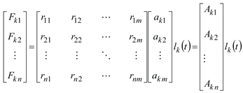
The coupling interface load can be expressed as a two-dimensional matrix with N rows and M columns characterized by time t and oil film thickness h. As shown in Eq. (1), Each row represents the size of the coupling interface load associated with the oil film thickness at a certain time point.
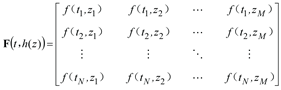 where is the coupling interface load. The spatial dimension is discretized into M discrete points, and the time dimension is discretized into N discrete points.
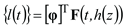
According to the POD decomposition principle [19], the covariance matrix R of the coupling interface load is first established, and then diagonalized , is the coordinate transformation matrix. By searching the orthogonal coordinate system, the projection of the coupling interface load vector on each coordinate axis is maximized, that is composed of the orthogonal basis selected by . φi,i = 1,2,3,⋯m is a set of standard orthogonal bases, representing the eigenmode matrix that only depends on space in the covariance matrix. Solving makes the mean square value of the principal coordinate which only depends on time take the stationary value on the eigen vector of the covariance matrix. And each stationary value is the eigenvalue D. Suppose that the eigenmode matrix in the covariance matrix which only depends on the space is regularized, the eigenmode matrix is defined as and the principal coordinate matrix is , Then the time-dependent principal coordinates of the space-time coupling interface load can be obtained by the following Eq. (2).
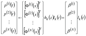
Thus, the coupling interface load is divided into the superposition of m sub-coupling interface loads, as shown in Eq. (3). The sub-coupling interface load is composed of the independent time history and the spatial distribution function.
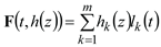 where is expressed as the k-th time history, is expressed as the k-th spatial distribution function.
2.2. Chebyshev Orthogonal Polynomial Fitting Spatial Distribution Function
Spatial distribution function can be approximated and fitted by a set of linearly independent functions. Chebyshev orthogonal polynomial [20,21] with excellent characteristics such as orthogonality and convergence are used to fit the spatial distribution function. First six specific forms of the Chebyshev polynomial of the first kind [22]. are , , and . Oil film thickness space of the coupling interface load is fitted with the m-term Chebyshev generalized polynomial; the Eq. (3) becomes as follows:
 where is the i-th Chebyshev orthogonal polynomial, is the coefficient before the i-th term Chebyshev generalized polynomial of the k-th distribution space function.
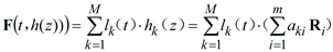
Then, a group sub-coupling interface load is equivalent to the concentrated load acting on the n limited action point of the sliding bearing-wind turbine gearbox shaft system. The equivalent concentrated load conversion is as follows:
 where , respectively represents the equivalent concentrated load and the equivalent amplitude coefficient coming from k-th group sub-coupling interface load equivalent to the n-th action point. is the equivalent amplitude coefficient coming from the i-th Chebyshev generalized polynomial function equivalent to the n-th action point.
Then, the coupling interface load composed of M group sub-distributed loads is converted to the n-th action point can be shown as Eq. (6).
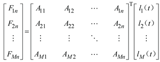 where , respectively represents the equivalent concentrated load and the equivalent amplitude coefficient coming from M-th group sub-coupling interface load equivalent to the n-th action point.
Through the Dop decoupling and Chebyshev polynomial fitting above mentioned, the coupling interface load is transformed into a series of concentrated loads acting on the limited points of the sliding bearing-wind turbine gearbox shaft system. Then, the conventional concentrated load transient response analysis method can be used to calculate the transient response under sliding bearing- wind turbine gearbox coupling interface load.
3. An improved Transient Response Analysis Method
3.1. modal Distribution
The dynamic differential equation of the wind turbine gearbox shafting system subjected to coupling interface load can be expressed as Eq. (7), which is similar to the concentrated dynamic load.
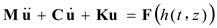 where, M, K and C represent the mass, stiffness, and damping matrices respectively. and ü,
  and u are the acceleration, velocity, and displacement responses of the wind turbine gearbox shafting, respectively.
and u are the acceleration, velocity, and displacement responses of the wind turbine gearbox shafting, respectively.Modal analysis [23] is essentially a coordinate transformation. From a computational view, the complex and coupled motion equations as Eq. (7) in the rational space are projected into the modal space by eigenvalue solution and modal transformation equation. The motion equations of a set of decoupled single-degree-of-freedom systems in the modal space are as follows:
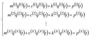 where, , and represent the i-order modal mass stiffness and damping respectively. and represent the corresponding modal displacement response and modal load, respectively. N is the number of structural degrees of freedom.
According to the modal transformation, the modal load shown in Eq. (7) and the k-th group sub-coupling interface load shown in Eq. (3) has the following form:
 where, represents ith-order modal shape of x position. is the inner product coming from the ith-order structure modal shape and Spatial distribution function , which is a constant.
It can be seen from Eq. (9) that each order modal loads have the same form of time history , but their amplitude coefficients are different.
3.2. Transient Response Analysis
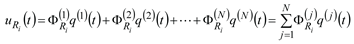
According to the modal superposition method, the response on the any freedom degree can be expressed as the superposition to the product of the modal response on each order and the modal shape coefficient. is the j-th order modal shape coefficient to the -th freedom degree.
Compared the Eq. (5) with Eq. (9), it can be found that the equivalent concentrated load equivalent for the sub-coupling interface load is the same as the modal load, and has the same form as the time history , but the coefficients are different. So, the transient response calculated by the concentrated load transient response analysis method [24] coming from the equivalent concentrated load is the same as that the transient response under the sub-coupling interface load, and there is a certain proportion . That is . Therefore, the concentrated transient response analysis method can be used to quickly evaluate the transient response of the wind turbine gearbox shafting under the coupling interface load and Provide displacement monitoring information.
In summary, the transient response analysis process under sliding bearing- wind turbine gearbox coupling interface load can be shown as the Figure 1.
4. Numerical Simulations
The sliding bearing-wind turbine gearbox shafting and corresponding finite element model (FEA) as shown in Figure 2, the shaft system is divided into 19 nodes with 18 units. The material properties are displayed as follows: the elastic modulus is 125GPa, Poisson ’s ratio is 0.335, the density is 8850kg / m 3. It is assumed that the coupling interface load is
 t ∈ [0,2] s, z ∈ [0,0.2]m with a diameter of 260 mm and a length of 200 mm is perpendicular to the left end of the shaft along the y direction.
4.1. Equivalented Sub-Coupling Interface Load
The coupling interface load is decoupled into the sub- coupling interface load with independent time history and spatial distribution function by the POD. When M = 3, the error is very small compared with the assumed coupling interface load. Figure 3 show the sub-coupling interface load combined linearly by independent time history and spatial distribution function. It can be seen from Figure 3 that the absolute error fluctuates between -100N and 100N, and the overall relative error is calculated to be only RE = 3.18E-5, which proves the accuracy and effectiveness of DOP to coupling interface load.
4.2. Spatial Distribution Function Fitting
The six term Chebyshev polynomials are used to fit the three groups spatial distribution functions h1(z), h2(z) and h3(z) shown in Figure 3. The coefficient aki is shown in Table 1. The relative errors shown in Table 1 and Figure 4 show that the fitted and uncoupled spatial distribution functions are consistent. The first and second group spatial distribution function show a linear function relationship, and the third group shows a quadratic function relationship. It shows that Chebyshev polynomials can fit the nonlinear space function with high precision.
4.3. Concentrated Load Equivalent
The six Chebyshev polynomials used to fit three group spatial distribution function are transformed into 1-5 nodes as shown in Figure 2 through the concentrated load equivalent finite element method [25], and the equivalent amplitude coefficients as can be obtained (shown in Table 2). According to the Eq. (5) and Eq. (6), the equivalent amplitude coefficients as is obtained by combining and shown in Table 1. they are shown in Table 2. Therefore, the three-group spatial distribution function of sub-coupling interface load are equivalent to the concentrated load acting on the shafting nodes 1-5. The five concentrated loads are respectively:
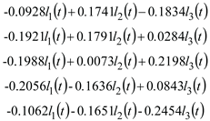
As shown in Figure 5, the three groups sub-coupling interface load are transformed into the concentrated loads at the five load points.
4.4. Transient Response Analysis
The equivalent concentrated loads acting on the 1-5 node are applied to the corresponding nodes respectively, and the displacement response (named as: concentrated response) on the node 6-11 under the time of 0-2s is obtained based on the concentrated load transient response analysis method. Compared together with the transient response (named as: coupled response) coming from coupling interface load and the linear superposition transient response (named as: superimposed response) coming from sub-coupling interface load based on the finite element analysis software [26], these results are shown in Figure 6. The coupled and superimposed response of displacement responses of the six nodes are equal, which proves the effectiveness of POD decomposition. That shows that the decoupled sub-coupling interface load can be used to replace the coupling interface load for transient response analysis to sliding bearing-wind turbine gearbox shafting system. There are the same vibration form and different amplitude coefficients between the concentrated response with coupled response. This relationship shows that the equivalent concentrated load can be used to quickly analyze the shaft displacement information.
5. Conclusions
Aiming at the problem that the time-space coupling interface load cannot directly call the conventional concentrated load transient response analysis method to calculate the displacement response of the wind turbine gearbox shaft system, this paper combines DOP decoupling and Chebyshev polynomials fitting to convert the coupling interface load into a series of concentrated loads. Numerical examples show that the superposition effect of displacement response under three sets of sub-coupling interface load coming from DOP is consistent with the displacement response under coupling interface load. Chebyshev polynomials can well fit the spatial distribution function in the sub-load. A series of equivalent concentrated loads can be used to quickly calculate the displacement response and provide displacement information for wind power fault diagnosis.
Data Availability Statement
The authors confirm that the data supporting the conclusion of the article are shown in the relevant Figure and tables in the article.
Acknowledgments
This work was conducted under funding by the National Natural Science Foundation of China (grant no.52375244); Hunan Provincial Natural Science Foundation of China (grant no.2023JJ30192); and Xiangtan Science and Technology Plan Key project (grant no. GX -ZD20221008).
Conflicts of Interest
The author(s) declared no potential conflicts of interest with respect to the research, authorship, and/or publication of this paper.
References
- Hu, C.C. Discussion on the present situation of wind power generation and the development of wind power industry. Sci. Technol. Innov. Prod. Forces 2023, 3, 55–57. [Google Scholar]
- Zhu, C.C.; Zhou, S.H.; Zhang, Y.B. Application status and development trend of sliding bearing in wind power gearbox. Wind Energy 2021, 9, 38–42. [Google Scholar]
- Jiang, R.; Teng, W.; Liu, X.B. Analysis and diagnosis of electrical corrosion of wind turbine generator bearings. China Electr. Power 2019, 6, 128–133. [Google Scholar]
- Wang, J.; Peng, Y.Y.; Qiao, W. Current-Aided Order Tracking of Vibration Signals for Bearing Fault Diagnosis of Direct-Drive Wind Turbines. IEEE Trans. Ind. Electron. 2016, 10, 6336–6346. [Google Scholar] [CrossRef]
- Pan, Q.B.; Cao, L.; Tang, Y.Y. Fault diagnosis technology and application of wind turbine bearing based on spectral kurtosis. Heilongjiang Electr. Power 2020, 5, 377–384. [Google Scholar]
- Su, G.L.; Wang, J.D.; Fu, E.Q. Application of XGBoost algorithm in fault monitoring and early warning of wind turbine generator. Sol. Energy 2021, 9, 78–84. [Google Scholar]
- Liu, G.Z.; Yu, Y.; Wen, B.C. Nonlinear Analysis of Rotor-stator-bearing System Unsteady Oil Film Force. Appl. Mech. Mater. 2013, 341–342, 399. [Google Scholar] [CrossRef]
- Wang, L.; Wang, M.; Hu, X. Oil film boundary analysis of spiral oil wedge sleeve bearing based on the dynamic loading conditions. Proc. Inst. Mech. Eng. Part J J. Eng. Tribol. 2017, 2, 254–262. [Google Scholar] [CrossRef]
- Ling, H.; He, L.L.; Zhang, P. Study on the law of oil film hole migration of sliding bearing under the fault of loose bearing. Mech. Des. Manuf. 2019, 2, 110–113. [Google Scholar]
- Yao, L.; Guo, W. Study on dynamic characteristics of single-span double-disk cracked rotor-bearing. Noise Vib. Control 2019, 5, 191–196. [Google Scholar]
- Song, L.R.; Cui, Q.W.; Zhou, J.X. Fatigue life and dynamic reliability analysis of high-speed shaft bearing of wind power gearbox. J. Sol. Energy 2023, 8, 437–444. [Google Scholar]
- Wei, W.; Guo, W.Y.; Wu, X.Y. Modeling and analysis of gear system considering time-varying dynamic parameters of sliding bearing. Vib. Shock 2019, 23, 246–252. [Google Scholar]
- Wang, W.B. Dynamic characteristic analysis of sliding bearing-rigid rotor system with flexible support. Mech. Transm. 2021, 6, 46–50. [Google Scholar]
- Cui, S.H.; Yan, W.M.; Liu, Q. The influence of acceleration mode on the start-stop processes of radial plain bearing. Bearing 2023, 1, 1–9. [Google Scholar]
- Wang, Y.J.; Yan, J.X.; Qi, X.Y. Study on dynamic characteristics of wind power gearbox bearing under variable working conditions. Fan Technol. 2023, 4, 49–54. [Google Scholar]
- Li, T.; Pan, T.Y.; Zhou, X.X.; Zhang, K.; Yao, J.Y. Non-Intrusive Reduced-Order Modeling Based on Parametrized Proper Orthogonal Decomposition. Energies 2023, 1, 1–22. [Google Scholar] [CrossRef]
- Zhang, G.J.; Yang, X.F.; Li, Y.; Gu, F.D. Numerical investigation on the cavitating wake flow around a cylinder based on proper orthogonal decomposition. Front. Energy Res. 2023, 11, 1–13. [Google Scholar] [CrossRef]
- Jia, X.Y.; Gong, C.L.; Ji, W.; Li, C.N. Flow sensing method for fluid-structure interaction systems via multilayer proper orthogonal decomposition. J. Fluids Struct. 2024, 124, 104023–104034. [Google Scholar] [CrossRef]
- Salman, S.; Sidra, T.M.L.; Muhammad, S.; Muhammad, R.; Abdul, W.B.; Syed, M.H. Reduced order model of offshore wind turbine wake by proper orthogonal decomposition. Int. J. Heat Fluid Flow 2020, 82, 108554. [Google Scholar] [CrossRef]
- Mohammad, P.; Marzieh, M.; Ali, A. Numerical estimation of the fractional Klein-Gordon equation with Discrete Chebyshev Polynomials. Alex. Eng. J. 2024, 90, 44–53. [Google Scholar] [CrossRef]
- El-Sayed, A.A.; Agarwal, P. Spectral treatment for the fractional-order wave equation using shifted Chebyshev orthogonal polynomials. J. Comput. Appl. Math. 2023, 424, 114933. [Google Scholar] [CrossRef]
- Griffin, J.; Mahmoud, S. Orthogonal rational functions arising from the Chebyshev polynomials of first and second kind. J. Math. Anal. Appl. 2023, 2, 126891–126922. [Google Scholar] [CrossRef]
- Zhen, Y.; Dai, C.W.; Cao, Z.Y.; Li, W.; Chen, Z.Z.; Li, C. Modal analysis and moving performance of a single-mode linear ultrasonic motor. Ultrasonics 2020, 108, 106216. [Google Scholar] [CrossRef]
- Liu, J.Y.; Chen, X.J.; Huang, H.; Ji, S.; Tu, Q.Z. A Simplified Method to Analyse Dynamic Response of VLFS Based on the Kane Method. Offshore Mech. Arct. Eng. 2022, 1, 1–18. [Google Scholar] [CrossRef]
- Zhan, Y.; Liu, C.S.; Zhang, F.P.; Qiu, Z.G. Experimental study and finite element analysis based on equivalent load method for laser ultrasonic measurement of elastic constants. Ultrasonics 2016, 69, 243–247. [Google Scholar] [CrossRef]
- Zheng, J.X.; Duan, Z.S.; Zhou, L.M. Finite element analysis and energy recovery calculation of carbon fiber composite based on ANSYS software. J. Appl. Biomater. Funct. Mater. 2022, 20, 1–23. [Google Scholar] [CrossRef]
Figure 1.
Transient response analysis process under coupling interface load.
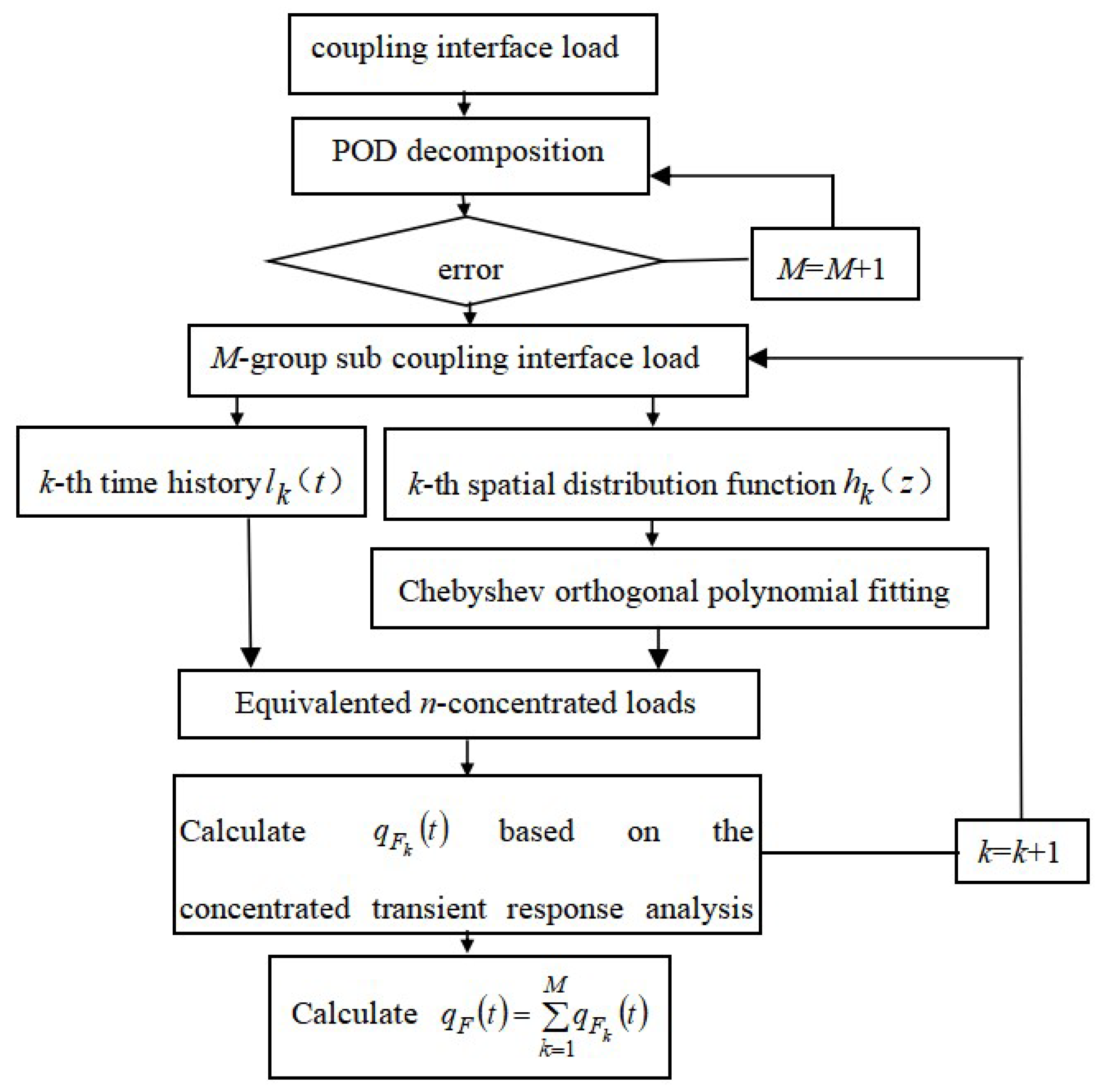
Figure 2.
Structure and FEA model.
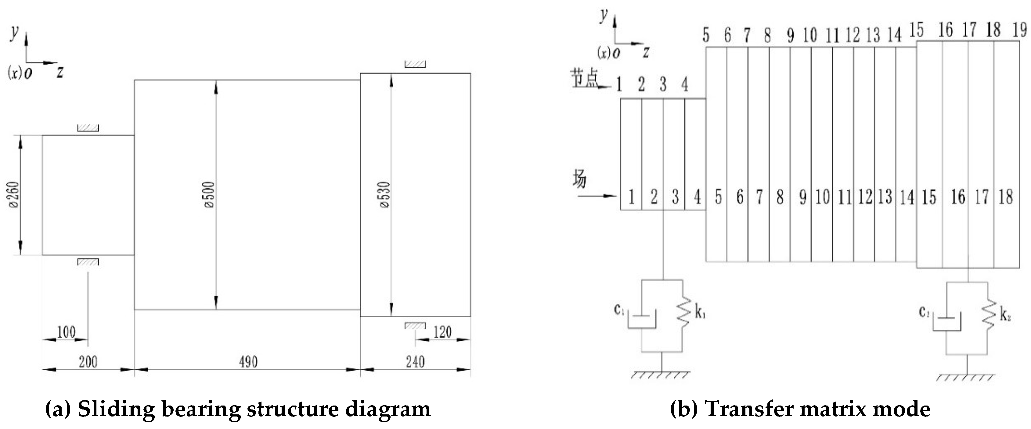
Figure 3.
The POD decomposition and error evaluation.
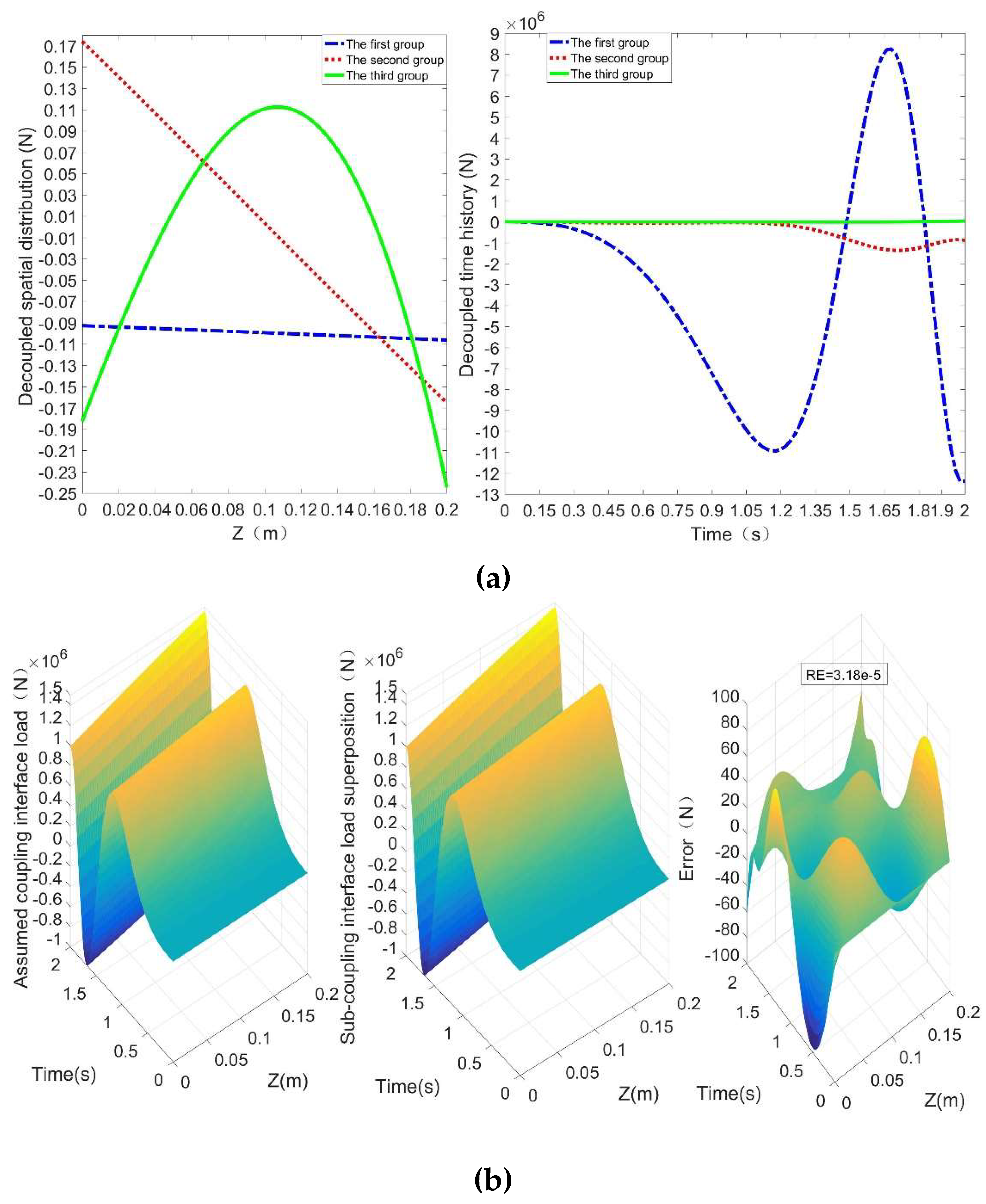
Figure 4.
Chebyshev fits three groups of oil film spatial distribution functions.
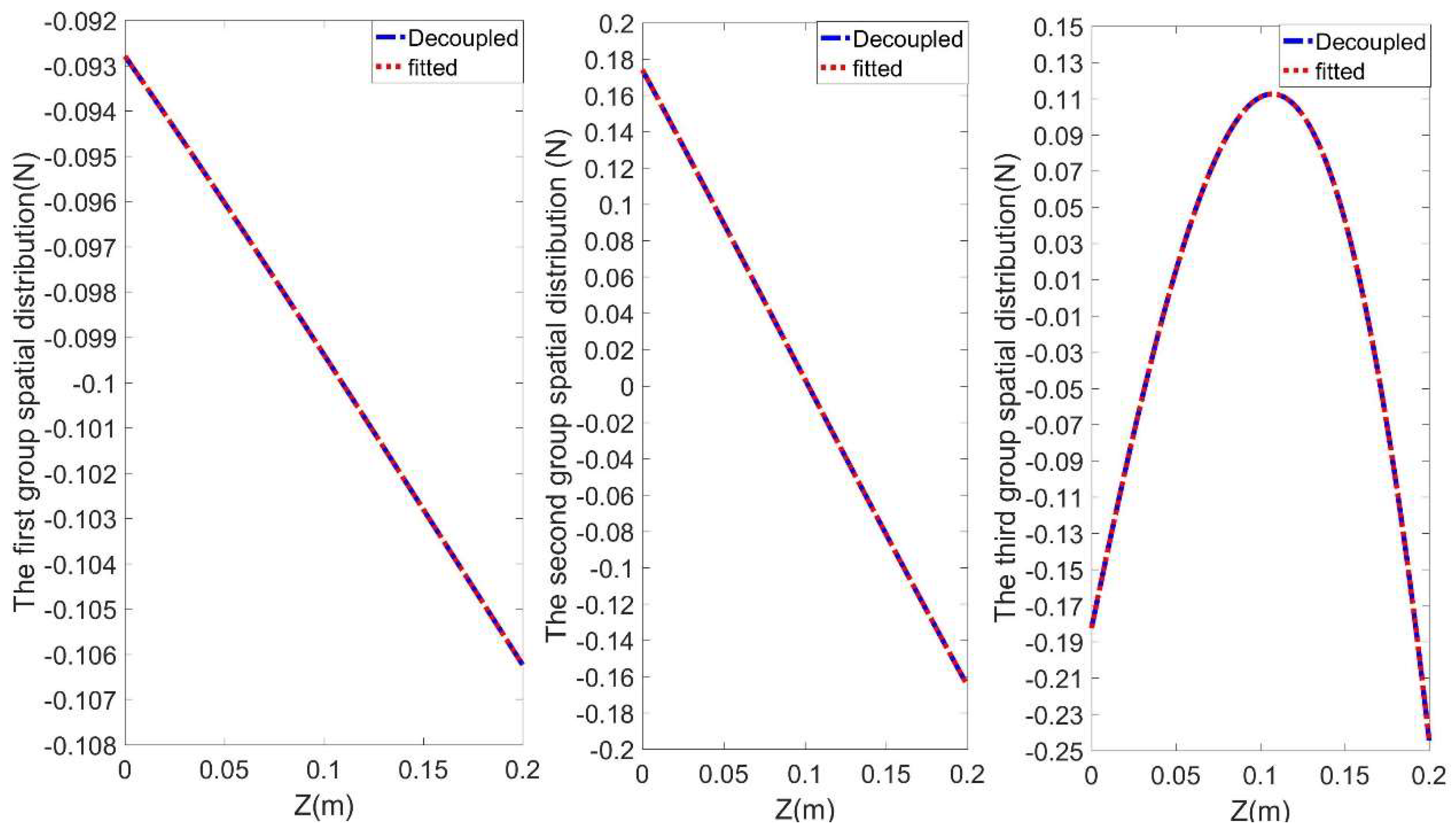
Figure 5.
Three-group sub-coupling interface load and equivalent concentrated loads.
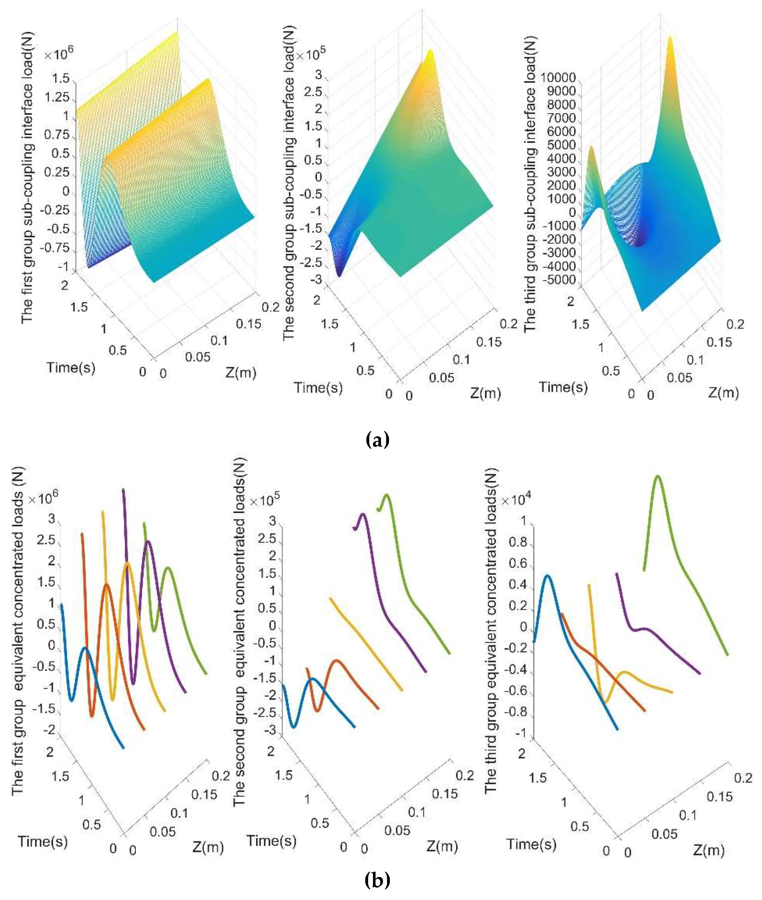
Figure 6.
Transient response analysis of coupling interface load, sub-coupling interface load and equivalent concentrated load.
Figure 6.
Transient response analysis of coupling interface load, sub-coupling interface load and equivalent concentrated load.
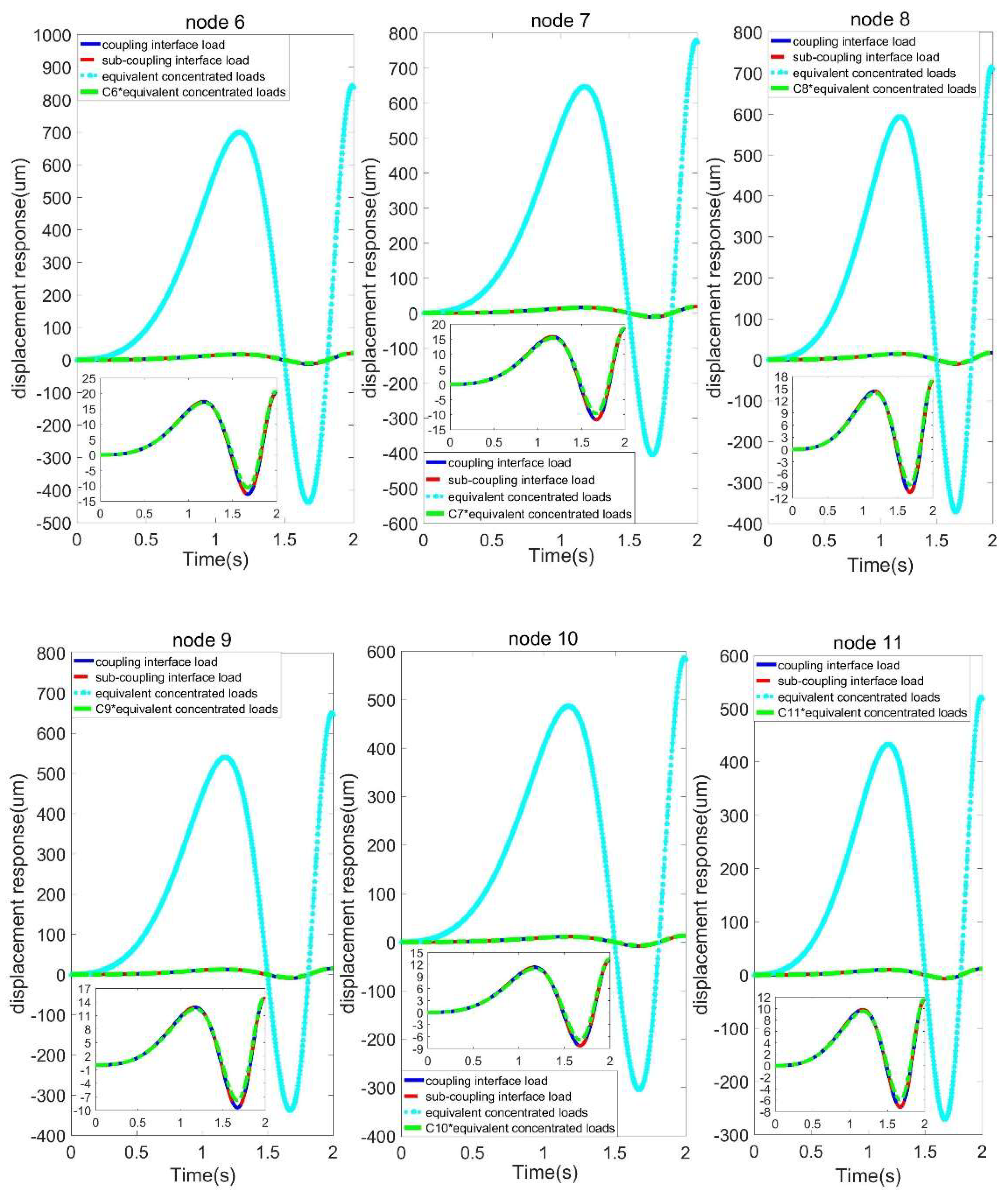

Table 1.
Coefficients before Chebyshev polynomial.
| Spatial distribution function | ak1 | ak2 | ak3 | ak4 | ak5 | ak6 | REK |
| h1(z) | -0.0994 | -0.0067 | -6.78E-05 | 1.67E-05 | -3.24E-07 | -2.89E-08 | 5.01E-09 |
| h2(z) | 0.0041 | -0.1702 | 0.0004 | 0.0006 | -7.62E-06 | -6.77E-07 | 1.17E-07 |
| h3(z) | -0.0518 | -0.0114 | -0.1622 | -0.0197 | 0.0004 | 4.15E-05 | 4.61E-06 |
Table 2.
Equivalent amplitude coefficient.
| n-load node | |||||||||
| 1 | 1 | -1 | 1 | -1 | -1 | -1 | -0.0928 | 0.1741 | -0.1834 |
| 2 | 2 | -1 | -1 | 2 | -5 | 1 | -0.1921 | 0.1791 | 0.0284 |
| 3 | 2 | -0 | -2 | 0 | -2- | 0 | -0.1988 | 0.0073 | 0.2198 |
| 4 | 2 | -1 | -1 | -2 | -5 | 1 | -0.2056 | -0.1636 | 0.0843 |
| 5 | 1 | 1 | 1 | 1 | -1 | 1 | -0.1062 | -0.1651 | -0.2454 |
Disclaimer/Publisher’s Note: The statements, opinions and data contained in all publications are solely those of the individual author(s) and contributor(s) and not of MDPI and/or the editor(s). MDPI and/or the editor(s) disclaim responsibility for any injury to people or property resulting from any ideas, methods, instructions or products referred to in the content. |
© 2025 by the authors. Licensee MDPI, Basel, Switzerland. This article is an open access article distributed under the terms and conditions of the Creative Commons Attribution (CC BY) license (http://creativecommons.org/licenses/by/4.0/).
Copyright: This open access article is published under a Creative Commons CC BY 4.0 license, which permit the free download, distribution, and reuse, provided that the author and preprint are cited in any reuse.


