Submitted:
30 May 2025
Posted:
02 June 2025
You are already at the latest version
Abstract
Since 1857, the second law of thermodynamics has faced the challenge of Maxwell's imagined demon. The widely accepted response to this challenge suggests that the demon requires a bit of information to function, and according to Landauer's principle, the erasure of this bit must offset the entropy reduction achieved by the demon. Recent studies involving two-state physical systems subject to thermal fluctuations at the nanoscale have aimed to either prove Landauer's principle or to demonstrate Szilard engines or Maxwell's demons in practice. We developed the equations and a numerical model to simulate the evolution of these systems. The results highlight the distinction between thermodynamic entropy and information entropy. They also demonstrate that Landauer’s principle has a limited range of applicability and that, using a two-state memory, it is possible to eliminate a small amount of entropy without expending energy—challenging the second law of thermodynamics.
Keywords:
entropy
; information
; Landauer's principle
; Maxwell’s demon
; second law
; Szilard engine
; thermal fluctuations
; Brownian motion
; bistable memory
; tilt memory
1. Introduction
Ludwig Boltzmann formulated the statistical version of the second law of thermodynamics, which he expressed in 1877 with the equation H = kB log W, where H is the entropy of a system, W is its statistical weight, and kB = 1.38 × 10⁻²³ J/K. A few years earlier, James Clerk Maxwell had developed the kinetic theory of gases and envisioned a demon capable of violating the second law [1]. In 1929, Leo Szilard [2] proposed a thought experiment involving an engine in which the entropy of a single molecule is reduced without expending energy, after detecting the molecule’s position. According to John von Neumann [3], it is the knowledge of the molecule’s position that enables an operator to achieve this reduction in entropy—a hypothesis that preserves the validity of the second law by establishing a link between information and entropy. In 1962, Rolf Landauer [4], building on Boltzmann’s formula, asserted that erasing a bit of information irreversibly generates an entropy of at least — a principle that has since gained wide acceptance.
Transient violations of the second law have long been observed in small systems, and it has been shown that they are consistent with fluctuation theorems [5] which apply to systems driven in a time-reversed manner. These apparent violations vanish when the results are averaged over many repeated identical experiments.
Since the 2010s, numerous experiments have been conducted at very low energy levels —on the order of at temperature — to support Landauer’s principle, implement a Szilard engine or a Maxwell’s demon, or explore the thermodynamics of two-state physical systems, which can be regarded as one-bit memories. These systems fall into two categories: bistable memories [6,7,8,9,10,11], characterized by an energy landscape with two minima, and tilt memories [12,13], which operate as all-or-nothing systems. In both cases, an actuator is used to alter the system’s potential energy. The stability of these memories is limited by thermodynamic fluctuations or quantum tunneling, which induce random transitions between states.
In a first article [14], we proposed an exploratory approach to several experiments, along with a brief overview of the historical connection between information and entropy. In a second article [15], we formulated the equations governing the quasistatic and out-of-equilibrium evolution of these systems, assuming the transition frequency is known as a function of the potential difference between the two states. We also suggested explaining apparent violations of the second law through a hypothesis on the temporality of entropy formulated by Landau and Lifshitz.
In the present article, we analyse recent experiments through two differents methods. First by computing the out-of-equilibrium evolution of bistable memories using the Langevin equation. Second, by directly derivating the equations for the quasistatic evolution of both bistable and tilt memories, starting from Gibbs’ formula for statistical entropy. Our analysis shows that thermodynamic entropy and information entropy do not always align and therefore cannot be regarded as equivalent. Landauer’s limit emerges in out-of-equilibrium processes but can be circumvented by slowing them to quasistatic regimes. We examined the arguments Landauer used to support his principle and identified a shortcoming in his reasoning. Finally, we analysed the behavior of these memory systems and the Szilard engines and Maxwell’s demons they can be used to implement, leading us to reveal a limitation of the second law at the nanoscale.
2. Results
2.1. Reset-to-Zero Operation of a Bistable Memory
In his 1961 paper [4], Landauer primarily referred to a bistable memory defined by a symmetric energy landscape (Figure 1, phase 1, and Figure 8 at t = 0), featuring two potential wells separated by a barrier that becomes more effective at hindering state transitions as its height increases. This type of memory has been realized, for example, by Bérut et al. [6] and Jun et al. [8], who used a colloidal particle in a liquid, subjected to a potential landscape created by an optical tweezer in the first study and by an electric field in the second. The particle’s movement is influenced by four factors: Brownian motion, friction, the gradient and the temporal variation of the potential.
We have thoroughly analysed the work of Jun et al., which yielded highly accurate results. The study began with a numerical simulation based on the Langevin equation to model the out-of-equilibrium evolution. The potential landscape U(x,t) applied to the particle is deterministic, but Brownian motion introduces considerable stochasticity to the system. We calculated the mean values of the variables over a large number of experiments, including the particle’s energy Us(t), the entropy S(t), and the probability P(t) of state 1. The work W done by the actuator and the heat Q transferred from the thermostat were derived from the changes in Us and S, with both quantities defined up to a constant. The simulation results align closely with the experimental data, demonstrating high accuracy.
We have developed a second approach by applying Gibbs’ formula for statistical entropy to derive the equations governing any quasistatic evolution of the system, allowing us to directly obtain the mean values of the variables. Both methods are described in detail in the Methods section.
They yield the same temporal evolution of the variables in quasistatic processes with high accuracy and produce identical results to those observed in the experiments of Jun et al. for both quasistatic and out-of-equilibrium processes. However, we disagree with their interpretation of the results, which will be discussed later.
In their experiment, the range of the potential is very large (from 13 to −40 , as shown in Figure 8). In contrast, we propose applying the equations to a simpler protocol where the potential varies between 0 and 13 and consists of three phases instead of four. This approach yields results that are much easier to observe and interpret. Both methods were applied to this protocol (Figure 1). The reset-to-zero occurs over three phases of equal duration. With a total duration of 900 s, we obtained the same result as Jun et al.’s experiment, which had a duration of 940 s. The initial potential landscape is a double parabolic well. First, the barrier is symmetrically lowered to create a single well with a flat bottom. This flat well then evolves into a parabolic well with a horizontal segment on the right. Finally, the horizontal segment is transformed into a parabolic well, returning the system to the initial double-well landscape.
At the start of phase 1, the memory state is randomly set to either 0 or 1 (indicating the particle is in the left or right well). For this example, we represent the initial state as 1. During phase 1, the barrier is lowered to create a flat-bottomed landscape, allowing the particle to move freely in a single well. In phase 2, the right side of the flat well is moved to the left, pushing the particle and confining it to a newly formed left well. Finally, in phase 3, the right well is restored while the particle remains in the left well.
Figure 2 shows the evolution of the key variables during the operation. The final work provided by the actuator is W = 0.71, matching the result from Jun et al.’s experiment and closely approaching Landauer’s limit of log2 = 0.693. The values of the probability P of state 1, heat Q, and work W are presented for both the simulation (subscript sim) and the quasistatic process (subscript qs). For the first two phases, the curves align perfectly. In the quasistatic limit, the actuator performs work W = 1.130 during the barrier lowering, but requires W = 1.823 to confine the particle in the left well, resulting in a total work W = log2.
In the simulation, if the third phase lasts the same duration as the first two, no heat or work is exchanged. The process is adiabatic, and the work done during the first two phases is not recovered. It has been dissipated, which appears to support Landauer’s principle. However, if we allow enough time for the third phase, it can also become quasistatic. As calculated in the Methods section, this duration is approximately 5 years. In this case, the work W is recovered, the entire process becomes reversible, and the reset-to-zero is not dissipative, which contradicts Landauer’s principle.
(sim = simulation of the experience for tc = 900 s, qs = quasistatic limit)
During phase 1, the probability P remains constant at P = 0.5. The memory receives heat Q ≈ 0.7 from the thermostat and transfers to the actuator work W ≈ 1.1. In phase 2, the work W increases to log2, while the heat Q decreases to −log2. During phase 3, the simulation shows no change, indicating an adiabatic process. However, in a quasistatic process, which requires an extremely long time, the work W is fully recovered, making the entire operation reversible.
2.2. Difference Between Information and Thermodynamic Entropy
Claude Shannon defined the information entropy of a one-bit memory by
, where P is the probability of either state.
In our experiment, we can compare it with the statistical entropy defined by Gibbs’ formula:
is the probability of the particle to be at abscissa at equilibrium (see the Methods).
During the reset-to-zero operation, we observe that H and S are equal at both the beginning and the end of the process but differ considerably in between (Figure 3). In phase 1, the probability of state 1 remains at P = 0.5, resulting in H = log2. However, as the barrier lowers, the phase space of the memory increases, causing S to increase to 1.403 in the quasistatic process.
This result challenges the commonly accepted equivalence between thermodynamic and Shannon entropies. Moreover, in the case of bistable memory, the choice of the boundary between states 0 and 1 is conventional. For a symmetric double well, it is typically placed along the axis of symmetry, though this is not a strict requirement. Changing the position of this boundary alters the Shannon entropy, while the thermodynamic entropy remains unaffected.
At the start of phase 1, . During phase 1, the state of the memory remains random (), while the statistical entropy increases to as the phase space expands. In phase 2, as the memory is pushed into state 0, both entropies decrease to 0.
If these two entropies are not equivalent, we must reconsider the arguments that Landauer used to establish his principle. He stated [4] that for a bit, a “well-defined initial state corresponds, by the usual statistical mechanical definition of entropy, , to zero entropy”. He further explained, “The degrees of freedom associated with the information can, through thermal relaxation, go to any one of possible states (for bits in the assembly), and therefore the entropy can increase by as the initial information becomes thermalized”. He writes that the reset-to-one operation of thermalized bits results in an entropy decrease of , and concludes that “The entropy of a closed system cannot decrease; hence, this entropy must appear somewhere else in the form of a heating effect”. The most widely stated form of his principle, which is equivalent to the original, asserts that erasing a bit causes an energy dissipation of at least .
Landauer applied the Boltzmann formula to a memory in a ‘well-defined state,’ meaning 0 or 1, which gives S = 0. However, he noted that after thermal relaxation, the entropy can increase to , acknowledging that this state is not at equilibrium. The limitation of Landauer’s approach was applying the Boltzmann formula to a ‘well-defined’ state of bistable memory, which is inherently out of equilibrium.
Finally, the experiment by Jun et al. does not prove Landauer’s principle. As in our simulation, if the duration of the final phase is long enough for the process to become quasistatic, the entire process becomes reversible, and the work W = log2 expended during the previous phases can be recovered. Therefore, the dissipation, which is often cited as evidence for Landauer’s principle, only occurs when the last phase is adiabatic and can be avoided if the phase is long enough to reach quasistatic conditions.
2.3. Shift Memory for an Energy-Neutral Reset-to-Zero
Using the same equipment employed to create the bistable memory — a colloidal particle in a fluid — we can design a different type of memory in which the information entropy is controlled and stable, without the need for a potential barrier. This concept is based on the zero-energy protocol introduced by Gammaitoni [16], leading to a single potential well that we propose to call shift memory.
The potential well is gradually shifted from left to right. The physical parameters of the memory (energy Us, entropy S) remain constant throughout. No work or heat is exchanged, but the probability of state 1 changes from 0 to 1, and the information entropy H fluctuates from 0 to log2 and back to 0. The operation is energy-neutral.
The single well can be shifted from one side to the other to invert the bit between states (NOT operation, Figure 4). When performed quasistatically, this operation is energy-neutral. In this process, the thermodynamic entropy remains constant, while the information entropy fluctuates from 0 to and back to 0.
For the shift memory, the reset-to-zero operation is also energy-neutral. If the initial state is 0, no action is needed. If the initial state is 1, it is inverted with zero energy. The initial position of the particle must be known to apply the protocol, so one possible counterargument is that the information about the position needs to be stored somewhere and erased after the operation. However, the information is already contained within the memory itself, and there is no need to copy and store it elsewhere. Therefore, this type of memory provides a direct challenge to Landauer’s principle.
2.4. Tilt Memory and Szilard Engine
A tilt memory is a physical system with two states, separated by a controlled potential difference . We refer to two sets of experiments on this type of memory. The experiments by Koski et al. [12] aimed at realizing a Szilard engine, involved a single-electron box. An electric potential difference applied between two metal islands influences the probability of an electron being present (state 1) or absent (state 0) in an intermediate region that forms the box.
The experiments of Ribezzi et al. [13] designed to create a Maxwell’s demon, used a ‘hairpin’ DNA fragment, where the two branches are linked by hydrogen bonds at rest (state 1) and can be separated by pulling on their ends (state 0). An actuator adjusts the electric potential in the first case and the traction force on the molecule in the second case to apply a potential difference between the two states.
In this case, unlike bistable memory, there is no degree of freedom to define the boundaries between states 0 and 1 of the one-bit memory. There is a logical correspondence between the physical and informational states, and we will observe that thermodynamic and Shannon entropy remains equal in this scenario.
Koski et al. [12] and Ribezzi et al. [13] used tilt memories to construct a Szilard engine, as illustrated in Figure 5. The energy landscape consists of two horizontal segments, with a potential of 0 for the left segment and a controlled potential U for the right segment.
In state A, the memory is randomly in state 0 or 1. When state 0 is detected, U is suddenly increased to a high value Um (phase 1), stabilizing the bit at 0. The statistical entropy Sst decreases from log2 to 0. In phase 2, U is gradually reduced back to 0, returning to the initial state. During this phase, heat Q = log2 is converted into work.
Initially, , and the memory bit is randomly set to either 0 or 1, with . The first phase begins when the memory is in state 0, after waiting as long as necessary. The potential is then abruptly increased to a value of , ensuring that state 0 becomes stable and . This process is adiabatic () and energy-neutral (). However, the system’s statistical entropy is now , having decreased by .
In phase 2, the potential is slowly reduced to 0, and the entropy returns to 0. The energy balance for this phase is and , from which we obtain , meaning that a quantity of heat was extracted from the thermostat, converted into work, and transferred to the actuator. These realizations of the Szilard engine demonstrate that it is possible to convert a quantity of heat into an equivalent amount of work, thus reducing the entropy of an isolated system, which contradicts the second law of thermodynamics.
The authors of these studies offered an interpretation to explain the entropy decrease without violating the second law. According to this interpretation, the information that the memory is in state 0, which triggers the cycle, is stored in an external memory. A quantity of entropy is generated when this information is erased, in line with Landauer’s principle. However, this argument no longer holds after the refutation of the principle.
Moreover, the information used to trigger the cycle resides within the memory itself; it is the bit corresponding to state 0. Therefore, there is no need to assume its storage and erasure outside of the memory.
2.5. Tilt Memory and Maxwell’s Demon
Ribezzi et al. [13] realized a Maxwell’s demon, the operation of which is illustrated in Figure 6. Initially, the energy level of the memory is with probability for state 1. The memory is typically in state 0, which is the most probable state. As soon as a transition to state 1 occurs, is suddenly driven adiabatically to a value << 0 to stabilize state 1, with the probability .
Then, during phase 2, it is returned quasistatically to its initial value . Experiment and theory (see Methods, Equation 12) show that the result of this operation is the transformation of heat into work , with a theoretically unlimited value.
In state A, the system can transition between state 0 (the most probable) and state 1. When state 1 is detected, the potential U is abruptly decreased to a very low value (phase 1 from A to B). This stabilizes the memory in state 1. During phase 2, the potential U is then gradually increased back to its initial value .
According to Ribezzi et al., this reduction in entropy is offset by the erasure of the information required to operate the process. This information would have been stored as an increasing number of bits during the waiting time of the first phase and then erased, dissipating energy in accordance with Landauer’s principle. However, as with the Szilard engine described earlier, this information resides within the memory itself, eliminating the need for external memory to store and erase it.
However, the local entropy reduction achieved within the system, as shown for the Szilard engine above, is far from being practically exploitable. In reality, the memory is part of an experimental setup that may include an optical tweezer with its laser beam, a cooling device, and other auxiliary equipment. In experiments of this type conducted to date, this setup generates much more entropy than it eliminates. Nonetheless, it remains true that the second law can be locally violated at energy levels on the order of .
2.6. Statistical and Thermodynamic Entropies
These two experiments – the Szilard engine and the Maxwell’s demon – present exceptions to the second law. They also highlight a distinction between thermodynamic and statistical entropies Sth and Sst, which arises from their definitions. For example, in state A of Figure 6, the energy landscape remains unchanged, so the statistical entropy Sst stays constant. However, each transition of the memory between state 0 and state 1 involves an exchange of heat and thermodynamic entropy, ΔQ = ΔSth = ± Ui, between the memory and the thermostat. As a result, the entropies Sth and Sst of the memory exhibit transient deviations.
3. Discussion
Since Szilard’s work, many physicists’ strong attachment to the absolute validity of the second law has led to some errors. We have demonstrated that it is possible to locally violate the second law at the nanoscale using Szilard engines and Maxwell’s demons, even though the experimental devices required to implement them currently generate far more entropy than they can eliminate.
We have also shown that the principle of equivalence between thermodynamic entropy and Shannon’s information entropy must be abandoned. Shannon [17] defined his entropy as the only mathematical function satisfying three well-defined constraints, which he encountered while solving cryptographic problems during the Second World War [16]. Starting from Hartley’s work [19], Shannon derived his formula for H to represent the minimum amount of information required to encode a given message. Its value depends on the frequency statistics within a specific context. Therefore, it is relative to that context, unlike the Gibbs formula, which applies to a well-defined physical system. While the two concepts are analogous, they apply to different domains.
Shannon’s formula is useful as a measure for information storage and processing. It has been reported [20] that von Neumann suggested the name “entropy” to Shannon for his statistical measure of information, which contributed to the widely accepted idea that there is an equivalence between thermodynamic and Shannon entropy [21].
We have pointed out experiments in which these entropies have different values. Moreover, they differ in nature. Thermodynamic entropy is a purely physical concept, whereas information entropy generally relies on a code — specifically, for bistable memory, it depends on a convention to define the boundary between the two states. Contrary to what Landauer asserted (“information is physical” [22]), information is immaterial and does not belong to the field of physics [23].
4. Methods
4.1. Simulation of Bistable Memory by Finite Difference Equations
In Jun et al.’s experiment [8], a particle was placed in water within a virtual potential U(x,t), which was updated every .
Between two updates, the particle experienced a force and underwent stochastic Brownian motion. The particle’s movement is governed by the Langevin equation, excluding the inertial term [24]:
where w is a white noise with mean and variance .
The friction coefficient is with N.s/m2 for water and the radius of the particle is r = 0.1 μm. Using the Einstein relation , we obtained μm2/s.
Thus, the displacement of the particle due to the potential gradient and the Brownian motion during is
During this displacement a heat transfer (positive or negative) occurs from the thermostat to the particle:
The potential landscape is then updated from to .
The total variation of the particle’s potential, considering Brownian motion, the potential gradient, and the action of the actuator, is given by the following:
Thus, according to the law of energy conservation, the actuator has provided work:
Using these finite difference equations, we can simulate the evolution of the memory by knowing the initial state x0 and U(x0,t0) along with function U(x,t). Due to the high stochasticity of Brownian motion, the variables must be averaged over a large number of trials.
We applied this method to the experiment of Jun et al., which yielded highly accurate results. The energy landscape is a quartic function of x, as shown in Figure 7 at the phase limits. The initial position of the particle is randomly chosen at the bottom of either the left or the right well. We allowed the system a period of 20 s to reach equilibrium.
We simulated runs from to (cycle time tc = 940 s). Thus,
For every simulation, we computed xi,j, Qi,j, Ui,j for indices , .
From x i,j, we obtained the mean probability of state 1 at time ti:
and the mean vectors: and .
With our units, the thermodynamic entropy is such that . Thus, if we take (for , we obtain
The experiment was designed to validate Landauer’s principle. The final result, both from the experiment and the simulation, yielded work W = 0.71 , which is in agreement with Landauer’s limit, log2. The evolution of the variables is shown in Figure 8 and Figure 9, where they are compared with the quasistatic values computed directly.
4.2. Quasistatic Equations of a Bistable Memory
The particle is confined between the abscissas xmin and xmax. The interval [xmin, xmax] is divided into N equal segments. For a quasistatic process, the probability of the particle being at abscissa at time t follows the Boltzmann distribution at equilibrium.
In the following, all variables depend on time t. The potential energy of the system is .
The statistical entropy is given by Gibbs’ formula, (Equation 6)
thus, or . (Equation 7)
The law of conservation of energy implies that . Based on our choice of units, Q and S vary identically as . Therefore, (Equation 8).
Given the initial state and , we could directly compute the numerical values of all relevant physical variables for a quasistatic process, as illustrated in Figure 8 and Figure 9. These computed values align closely with the simulation results, except at the end of phase 4, which is not quasistatic in the experiment.
The agreement between these two independently derived methods — and their consistency with the final result of the experiment by Jun et al. — strongly supports the validity of both approaches.
Thus, we can apply them to a simpler protocol, which is more convenient to illustrate the basic process in action.
The simulation values W and U fit perfectly with the quasistatic values
(W is deterministic, U fluctuations are not visible at this scale).
The simulation values Psim and Qsim differ from quasistatic values only by fluctuations during the first 3 phases but diverge at the end of phase 4, which is adiabatic.
4.3. Application to a Simpler Protocol
In Jun et al. [8], the potential could vary between 13 and −40 kBT during the operation. These important variations make it difficult to visually follow the values of the main parameters.
We propose a simpler protocol that can be implemented using the same equipment, featuring a potential variation between 0 and 13 kBT and a total duration of 900 s, divided into three equal phases instead of 940 s divided into four phases. This protocol yields the same final results and is easier to interpret. It is shown in Figure 1, with the evolution of the system variables illustrated in Figure 2 and Figure 3.
The energy landscape is a continuously differentiable function composed of quadratic segments of the form , where for the wells, a = 0 for the steps, and a = ±54 for the junctions, to ensure continuity of the derivatives. During each phase, the potential evolves through linear interpolation between its values at the beginning and at the end of the phase.
The distance between the two minima is Δx = 2.4 μm, and the maximum potential of the barrier or the steps is . The boundary between state 0 and state 1 is set along the axis of symmetry of the figure.
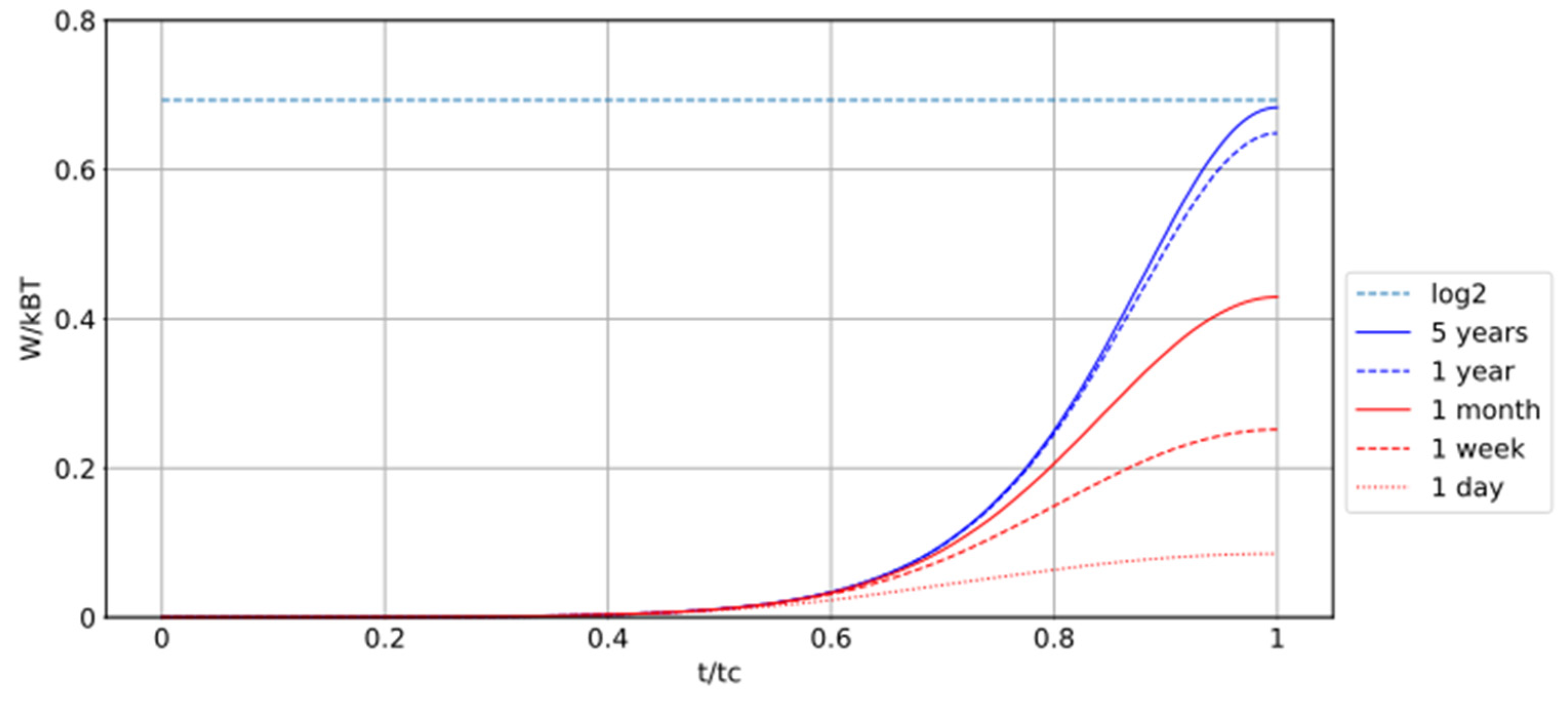
What is the duration for a quasistatic last phase?
We observed that if the last phase was quasistatic, the energy could be recovered. What would be the time necessary for that phase to be quasistatic? We have computed it using Kramers’ law [15].
The hopping frequency given by Jun et al. for this situation is , where ΔU is the height of the barrier to overcome and .The differential equation describing the probability of being in state 1 is . (Equation 9)
In our case and .
Kramers’ formula becomes highly approximate when the barrier height is low, which occurs at the beginning of phase 3 in state 1. However, as shown in Figure 2, W and Q remain constant during most of phase 3, so this approximation has no impact in this case.
The numeric integration of Equation 5 for several time scales of last phase gives the results shown in Figure 10.
During the experiment, the result is W 0 (for t = 300 s). One needs approximately 5 years for the process to be quasistatic and reversible to recover W = log2.
4.4. Quasistatic Equations for Tilt Memory
The quasistatic equations for tilt memory, inferred from the previous equations of bistable memory with , are the following:
, equivalent to or , (Equation 11)
, and
.
Notably, we have in this case .
From Equations 10 and 11, we obtain .
Then, from Equation 9, we obtain . (Equation 12)
4.5. Application to Maxwell’s Demon
In the Maxwell’s demon setup represented in Figure 6, the memory initially has an energy level of with as the probability of state 1. As soon as a transition to state 1 occurs, is suddenly and adiabatically lowered to << 0 to stabilize state 1 with . The work required for this phase is .
Then, it is returned quasistatically to its initial value . The work necessary for the second phase is
Thus,
As , we finally obtained or (Equation 13)
Data and Code Availability
The simulation model (Python) presented in this paper is available from the author upon reasonable request.
Data Availability Statement
Lead contact. Further information and requests for resources and reagents should be directed to and will be fulfilled by the lead contact, Jean Argouarc’h (jr.argouarch@gmail.com).
Conflicts of Interest
The author declares no competing interests.
References
- Leff, H., and Rex, A. (2003). Maxwell’s Demon 2: Entropy, Classical and Quantum Information, Computing Institute of Physics. (Institute of Physics).
- Szilard, L. (1929). On the decrease of entropy in a thermodynamic system by the intervention of intelligent beings. Syst. Res. 9, 301–310.
- von Neumann, J. (1932). Mathematical Foundations of Quantum Mechanics (Princeton University Press).
- Landauer, R. (1961). Irreversibility and heat generation in the computing process. IBM J. Res. Dev. 5, 183–191. [CrossRef]
- Ritort, F. Work fluctuations, transient violations of the second law and free-energy recovery methods: Perspectives in Theory and Experiments. In (Poincaré Seminar 2 (2003) 195–229). [CrossRef]
- Bérut, A., Arakelyan, A., Petrosyan, A., Ciliberto, S., Dillenschneider, R., and Lutz, E. (2012). Experimental verification of Landauer’s principle linking information and thermodynamics. Nature 483, 187–189.
- Orlov, A.O., Lent, C.S., Thorpe, C.C., Boechler, G.P., and Snider, G.L. (2012). Experimental test of Landauer’s principle at the sub-kbT level. Jpn. J. Appl. Phys. 51, 06FE10. [CrossRef]
- Jun, Y., Gavrilov, M., and Bechhoefer, J. (2014). High-precision test of Landauer’s principle in a feedback trap. Phys. Rev. Lett. 113, 190601.
- Hong, J., Lambson, B., Dhuey, S., and Bokor, J. (2016). Experimental test of Landauer’s principle in single-bit operations on nanomagnetic memory bits. Sci. Adv.
- Gaudenzi, R., Burzurí, E., Maegawa, S., Zant, H.S.J. van der, and Luis, F. (2017). Quantum-enhanced Landauer erasure and storage of molecular magnetic bit. 13th International Workshop on Magnetism and Superconductivity at the Nanoscale.
- Dago, S., Pereda, J., Barros, N., Ciliberto, S., and Bellon, L. (2021). Information and thermodynamics: fast and precise approach to Landauer’s bound in an underdamped micromechanical oscillator. Phys. Rev. Lett. 126.
- Koski, J.V., Maisi, V.F., Pekola, J.P., and Averin, D.V. (2014). Experimental realization of a Szilard engine with a single electron. Proc. Natl. Acad. Sci. USA 111, 13786–13789.
- Ribezzi-Crivellari, M., and Ritort, F. (2019). Large work extraction and the Landauer limit in a continuous Maxwell demon. Nat. Phys. 15, 660–664.
- Argouarc’h, J. (2021). Information-entropy equivalence, Maxwell’s demon and the information paradox. Available online: https://www.openscience.fr.
- Argouarc’h, J. (2022). Paradox of entropy: a bit of Information without energy. Available online: https://www.openscience.fr; https://www.openscience.fr/Paradox-of-entropy-a-bit-of-Information-without-energy.
- Gammaitoni, L. (2021). The Physics of Computing (Springer International Publishing). [CrossRef]
- Shannon, C. (1948). A mathematical theory of communication. Bell Syst. Tech. J. 27, 379–423.
- Shannon, C. (1945). A Mathematical Theory of Cryptography (Alcatel-Lucent).
- Hartley, R. (1928). Transmission of information. Bell Syst. Tech. J. 7, 535–563.
- Tribus, M. (1971). Energy and information. Sci. Am.
- Brillouin, L. (1959). La science et la théorie de l’information Jacques Gabay.
- Landauer, R. (1991). Information is physical. Physics Today 44, 23–29. [CrossRef]
- Argouarc’h, J. (2020). Archéologie du signe: Théorie unifiée de l’information et de la connaissance (L’Harmattan).
- Volpe, G., and Volpe, G. (2013). Simulation of a Brownian particle in an optical trap. American Journal of Physics 81, 224–230. [CrossRef]
Figure 1.
Reset-to-zero operation of a bistable memory.
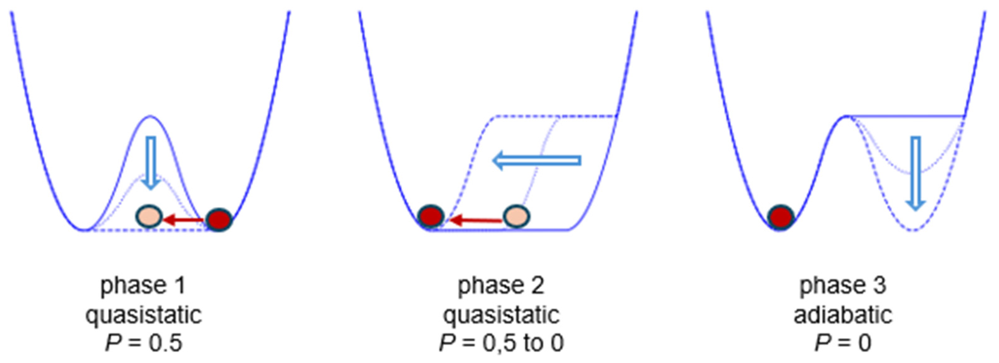
Figure 2.
Evolution of the variables during reset-to-zero operation.
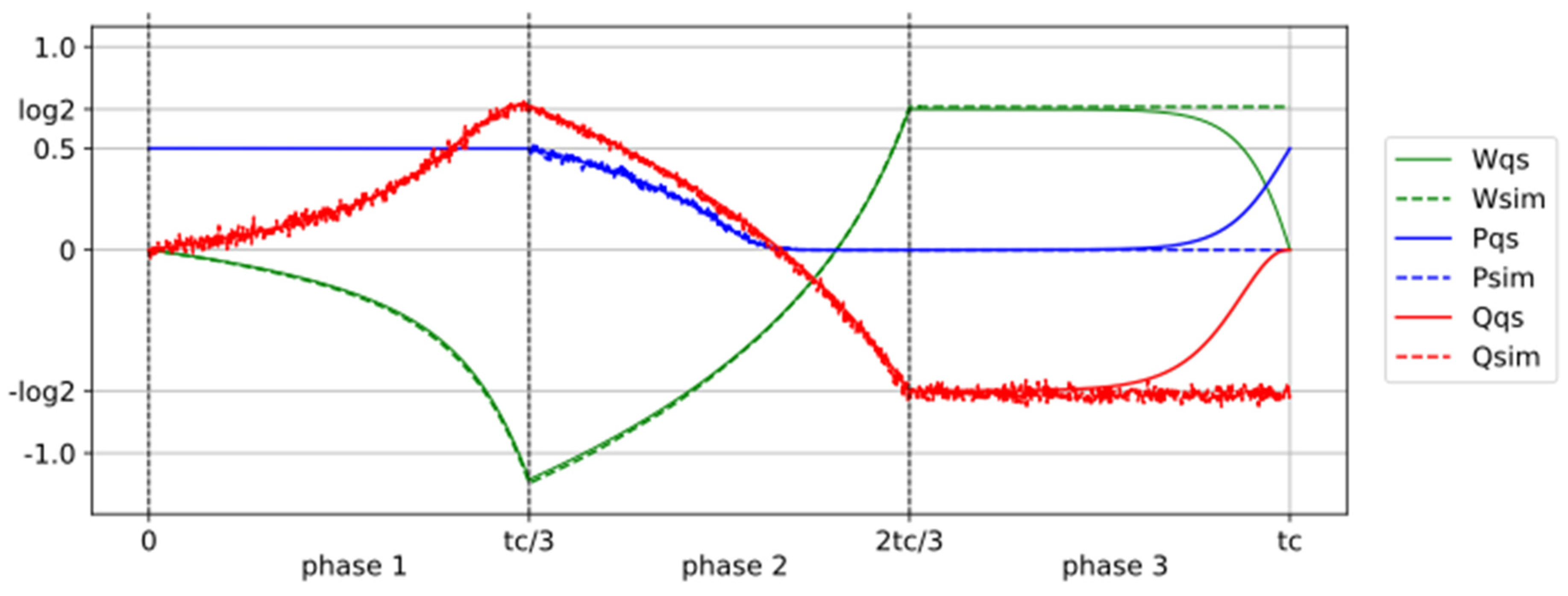
Figure 3.
Statistical entropy vs. information entropy at the quasistatic limit.
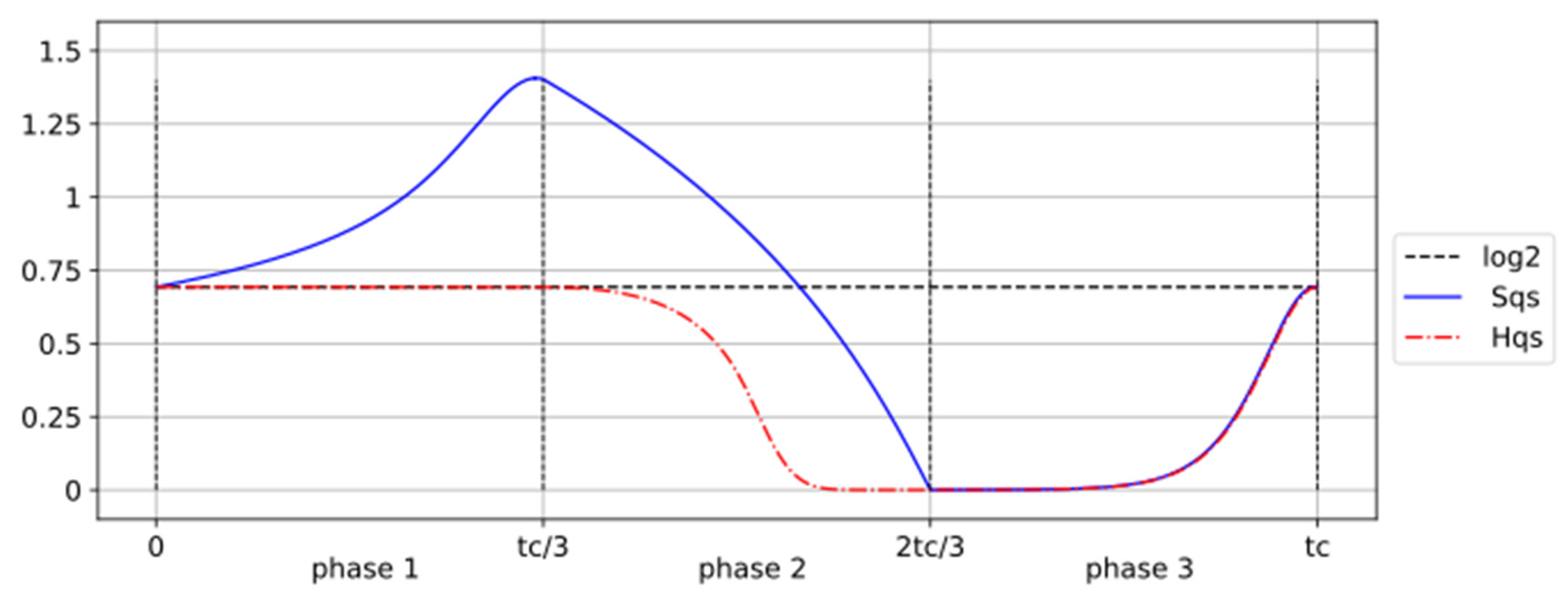
Figure 4.
NOT operation with shift memory.
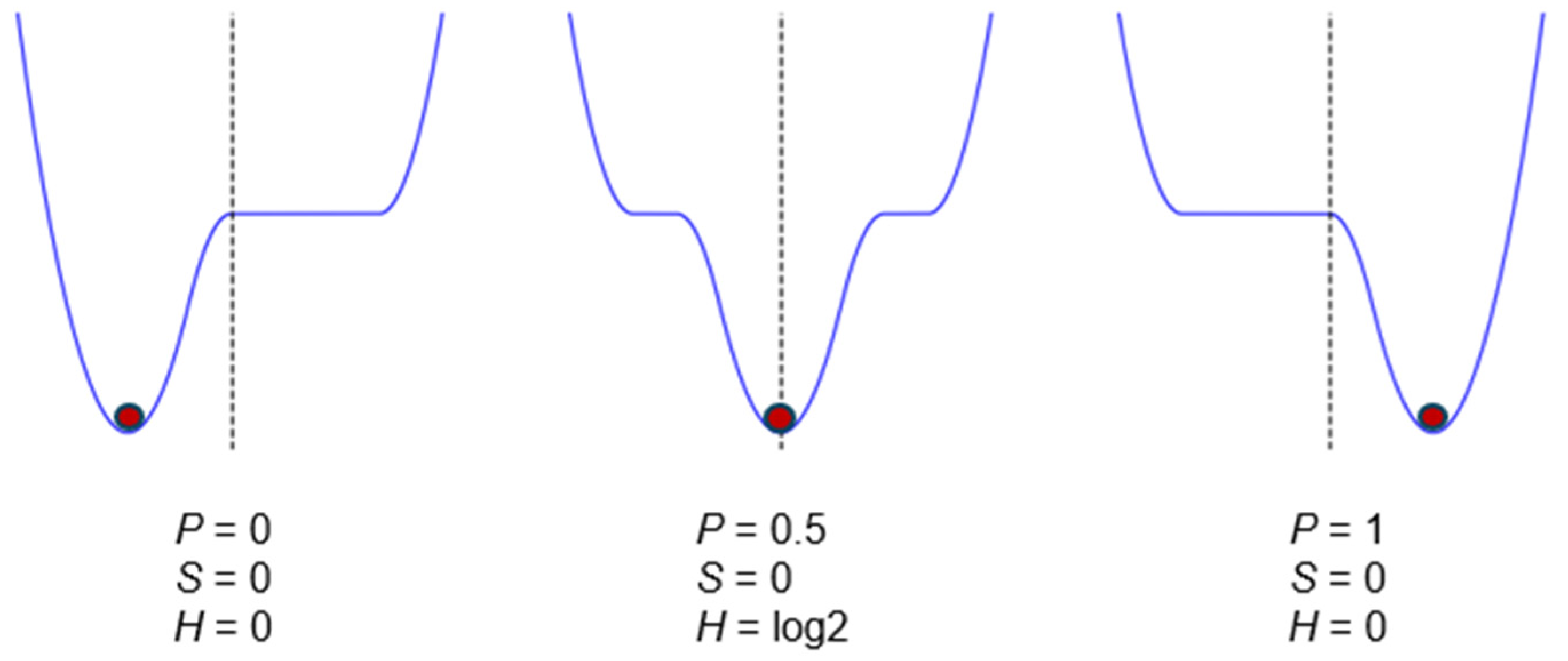
Figure 5.
A Szilard engine.
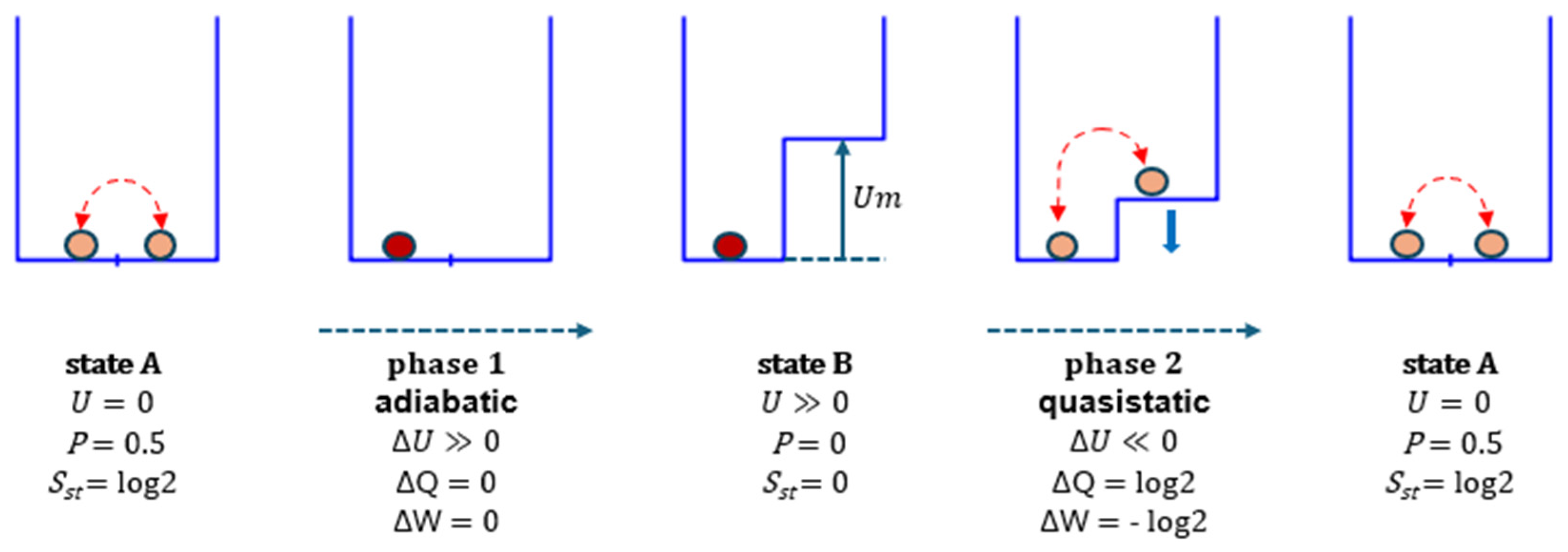
Figure 6.
A Maxwell’s demon.
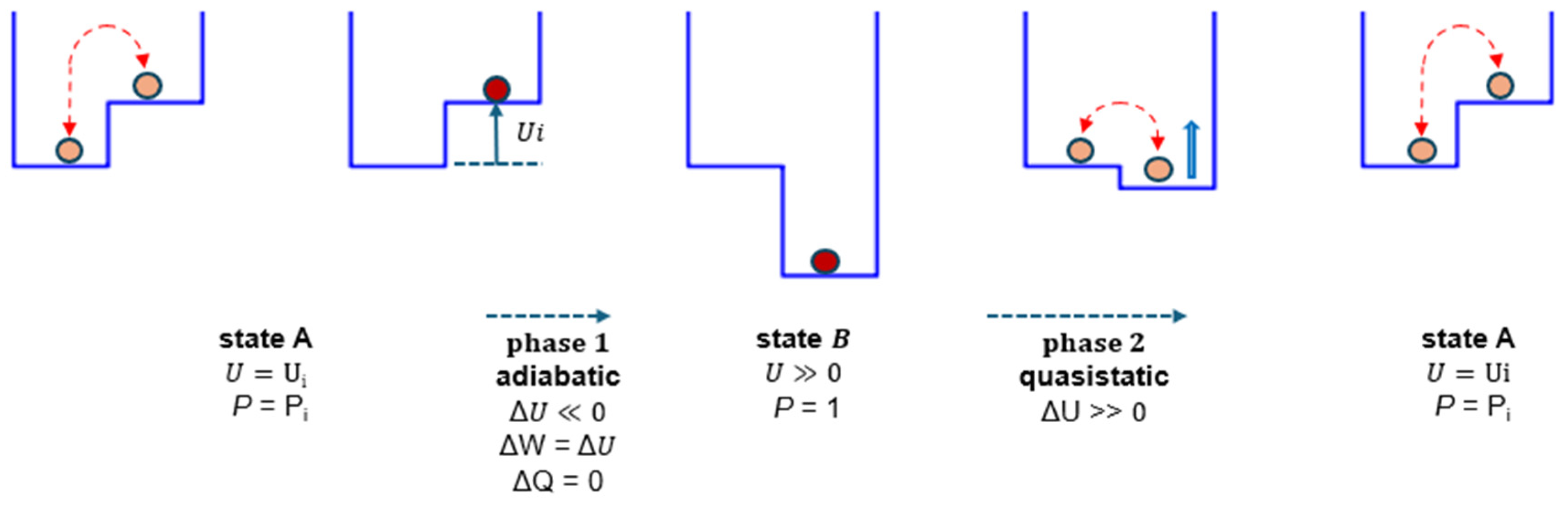
Figure 7.
Energy landscape at phase limits. At the end of phase 4, the profile returns to its original shape (t = 0).
Figure 7.
Energy landscape at phase limits. At the end of phase 4, the profile returns to its original shape (t = 0).
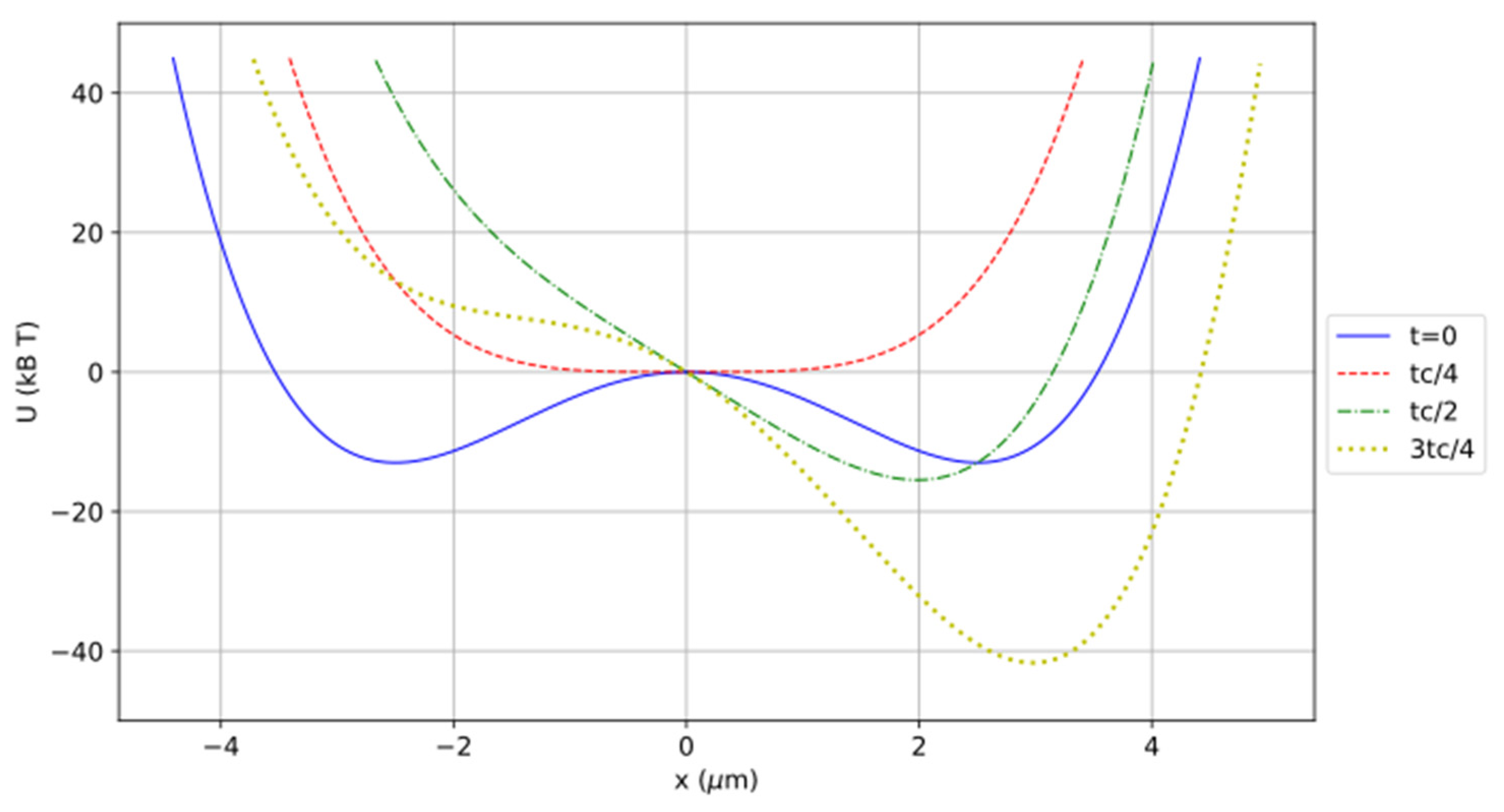
Figure 8.
Evolution of work W and potential U of the particle.
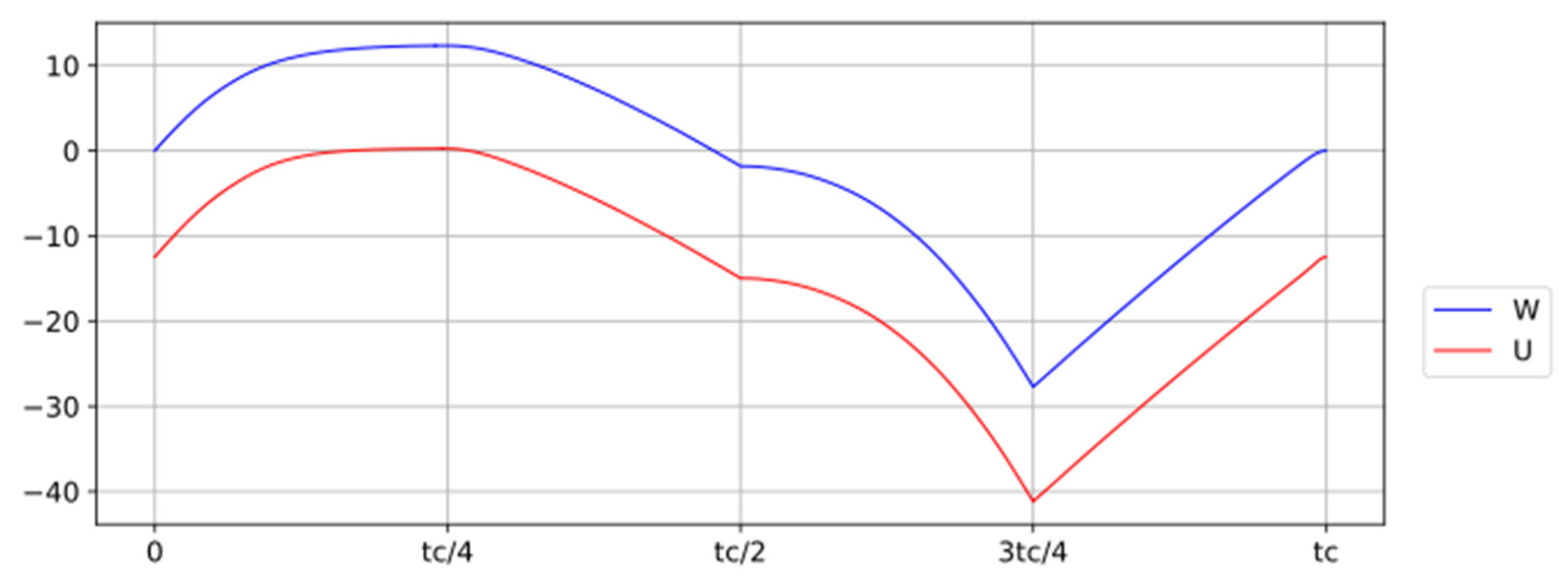
Figure 9.
Evolution of P and Q.
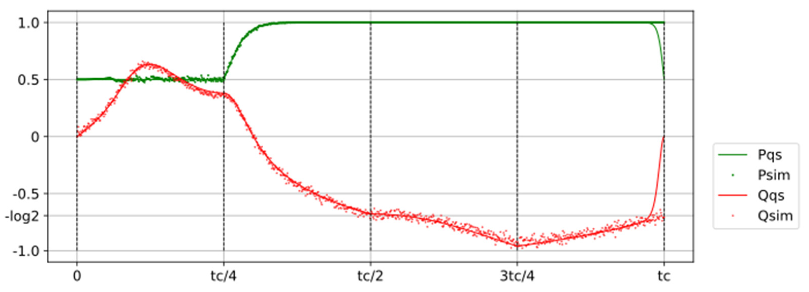
Figure 10.
Energy W recovered by the actuator during the last phase as a function of its duration tc up to 5 years.
Figure 10.
Energy W recovered by the actuator during the last phase as a function of its duration tc up to 5 years.
Disclaimer/Publisher’s Note: The statements, opinions and data contained in all publications are solely those of the individual author(s) and contributor(s) and not of MDPI and/or the editor(s). MDPI and/or the editor(s) disclaim responsibility for any injury to people or property resulting from any ideas, methods, instructions or products referred to in the content. |
© 2025 by the author. Licensee MDPI, Basel, Switzerland. This article is an open access article distributed under the terms and conditions of the Creative Commons Attribution (CC BY) license (https://creativecommons.org/licenses/by/4.0/).
Copyright: This open access article is published under a Creative Commons CC BY 4.0 license, which permit the free download, distribution, and reuse, provided that the author and preprint are cited in any reuse.


