
Submitted:
27 May 2025
Posted:
28 May 2025
You are already at the latest version
Abstract
The article presents a 3D mathematical modeling of the influence of electrical inhomogeneity of the ion-exchange membrane surface on the processes of salt ion transfer in membrane systems with axial symmetry, in particular, an annular membrane disk. This model is presented as a boundary value problem for the coupled system of Nernst – Planck – Poisson and Navier – Stokes equations in a cylindrical coordinate system. A hybrid numerical-analytical method for solving the boundary value problem is proposed, and the results for the annular disk model obtained by the hybrid method and the independent finite element method are compared. The applicability areas of each of these methods are determined. The main patterns and features of the occurrence and development of electroconvection associated with the electrical inhomogeneity of the membrane disk surface are determined using the example of an annular membrane disk. In particular, it is shown that electroconvective vortices arise at the junction of conductivity and non-conductivity regions at a certain ratio of the potential jump and angular velocity. Electroconvective vortices flow down in the radial direction to the edge of the annular membrane. At a fixed jump in potential, greater than the limiting value, the formed electroconvective vortices gradually decrease with increasing angular velocity of rotation until they disappear. And vice versa, at a fixed value of angular velocity of rotation, electroconvective vortices arise at a certain jump in potential and with its subsequent increase gradually increase in size.
Keywords:
hybrid numerical-analytical method
; axial symmetry
; electrical inhomogeneity
; electroconvection
; ion transport
; membrane systems
; overlimit mass transfer
1. Introduction
Operation of electromembrane systems (EMS) in overlimit current modes has a significant potential for a significant reduction in investment costs for desalination plants. The study by Wessling M., Stockmeier F. et al. [1] is devoted to the analysis of electroconvective vortices using the surface patterning method or geometric and electrical heterogeneity. In [1], a comparison of electroconvection development on two membranes modified using patterns was performed. An analysis was carried out of the increase in the area of electroconvective vortices, their structural stability in a steady state, as well as the possibility of controlling electroconvective vortices by introducing certain structural heterogeneities of the membrane surface to reduce energy losses in the current-voltage characteristic (CVC) and more economical operation in EMS in overlimit modes, significantly increasing their efficiency.
As the analysis of works [2,3,4,5] shows, the phenomenon of overlimit mass transfer is currently being intensively studied, however, many issues are still poorly understood. For example, it is necessary to study what effect modifications of the membrane surface have on the development of electroconvection. Electrical inhomogeneity arises due to the inhomogeneous distribution of charges on the membrane surface, which can be caused by both the geometric features of the system [6,7] and the properties of the membrane material. In work [8], it is shown that such inhomogeneities lead to local zones with increased electric field strength, which, in turn, affects the rate of ion migration, and, accordingly, the emergence and development of electroconvective vortices. This, in turn, leads to an increase in the rate of ion transfer through the membrane. In works [9,10,11,12], the importance of taking into account electrical inhomogeneity in modeling ion transport is also emphasized.
In recent years, there has been significant progress in understanding the role of electrical heterogeneity and electroconvection in EMS. A new model was proposed in [13] that takes into account nonlinear effects in electroconvection, which allowed for a more accurate description of mass transfer processes under high current density conditions.
Experimental studies conducted in [14] confirmed that taking into account electrical heterogeneity allows for a more accurate description of mass transfer processes in membrane systems. Theoretical models developed on the basis of these data take into account both ion migration and convective flows, which makes them more realistic.
Thus, the study of electrical heterogeneity and its effect on ion transport with electroconvection taken into account is an important area of research into increasing the efficiency of separation and purification of solutions and is of great practical importance. Further theoretical research in this area should be aimed at developing more accurate models. The advantage of constructing 3D models with axial symmetry is the property of equal accessibility at sublimiting currents, i.e. the fact that the thickness of the diffusion layer in such systems is constant up until the moment of the onset of electroconvection. At the same time, we note the insufficient development of such mathematical models and numerical methods for solving boundary value problems for overlimit current modes.
This article is a continuation of the work [15], where the basic 3D model of electroconvection with axial symmetry was formulated and investigated. In this article, a modification of the basic model in the form of an annular membrane disk is considered, associated with the addition of non-conductivity areas on the cation-exchange membrane (CEM) and their influence on the transfer process is investigated.
2. Methods
2.1. Mathematical Model of Transport for Annular Membrane Disk
Let us consider the transfer of salt ions during rotation of a cation-exchange membrane disk, with non-conducting and conducting regions, inside a vertically standing cylindrical cell around the central axis, taking into account electroconvection, and formulate the corresponding mathematical model.
2.1.1. Solution Area
When formulating a mathematical model, as well as the subsequent numerical solution due to axial symmetry (Figure 1a), it is sufficient to describe half of the cross-section of the cylindrical region, where it is necessary to determine the equations and boundary conditions (Figure 1b). To do this, it is necessary to move from a rectangular coordinate system to a cylindrical one . However, the velocities in the angular direction dffer from zero, so the model must include all three components of velocity (radial, azimuthal and axial), flows, electric field strength, although they depend only on two arguments , i.e. we have a 2D model. Moreover, with axial symmetry, the derivatives with respect to the component are zero, so all equations in the cylindrical coordinate system can be simplified in this case.
2.1.2. System of Equations
To model the transfer processes, a coupled system of Navier – Stokes equations with volumetric electric force and Nernst – Planck – Poisson equations is used, which in a cylindrical coordinate system takes the form [15]:
Where
, where – radial, azimuthal and axial components of the solution flow velocity ; index 1 refers to cations, index 2 to anions; – flows; - concentration in solution; – charge numbers; – current density; – diffusion coefficients; – electric field potential; – electric field strength; – dielectric permeability of the electrolyte; – Faraday constant; – universal gas constant; – absolute temperature; – time; – density; – dynamic viscosity and – pressure.
2.1.3. Boundary Conditions
In the studied section of the cylindrical region (Figure 1), boundary 2 models the part of space infinitely distant from CEM, in which the condition of electroneutrality is satisfied and the concentration of the solution is constant (). Boundary 2 is also considered an anode and an open boundary (inlet) for the solution, for the velocity here the condition of the absence of normal voltage is set, and the pressure is considered equal to zero. This boundary is considered an equipotential surface, and . Boundary 1 is the axis of symmetry. Boundary 5 is considered the outlet for the solution, therefore the condition of removal of ions only by convective flow is set , and for the velocity the condition of absence of normal stress. In addition, for the potential the boundary condition is used , here is the normal vector. At boundary 4 the CEM surface is considered equipotential: . Boundaries 3, 4 correspond to the rotating CEM, for the azimuthal velocity the condition is used here: , where is the angular velocity of rotation of the disk. For anions the condition of impermeability (absence of flow) is set here: . The conductivity region is located at boundary 4, so the cation exchange membrane forms a ring (Figure 1b). At boundary 3, corresponding to the non-conducting region, there is a condition of impermeability (no flow): , . To derive the condition for the potential at the non-conducting boundary 3, the equality of the current density to zero at this boundary is used. The normal component of the current density at this boundary is equal to zero due to the conditions on the flows. We determine the radial component of the potential gradient from the condition that the radial component of the current density is equal to zero from the formula for the current (4):
Therefore, from , we get:
Since the radial component of the velocity is , we obtain:
From here: .
Thus, at boundary 3, the following condition must be set for the potential:
It is assumed that the cell is initially completely filled with an ideally mixed solution of sodium chloride with a concentration and the same ideally mixed solution is fed into it through the boundary 2. Therefore, a constant concentration is taken as the initial condition .
2.2. Algorithm for Hybrid Numerical-Analytical Solution
2.2.1. Problems of Numerical Solution of Boundary Value Problem
In order to clarify the problems of numerical solution of the boundary value problem, we will move to a dimensionless form using characteristic quantities.
The problem has two characteristic quantities - the cell height and is the outer radius of the annular membrane. Since in practice , where proportionality coefficient , therefore they have the same order, and is taken as a characteristic quantity, since it is convenient to express the characteristic speed through it. As the characteristic velocity , we will use the azimuthal component of the velocity V0 = ω0r0.
Let us assume that:
Next, we will make the transition in the equations from dimensional quantities to dimensionless ones. Then we will get:
where
Let us evaluate and clarify the meaning of dimensionless parameters. The system of Nernst – Planck – Poisson and Navier – Stokes equations in a cylindrical coordinate system obtained in the process of non-dimensionalization includes 4 dimensionless parameters:
1. The Peclet number shows the ratio of the coefficients of kinematic viscosity and diffusion. With a characteristic channel height and an outer radius of the membrane disk of 1 mm, we obtain an estimate of the Peclet number (Table 1):
The Peclet number can be considered a large parameter, that is, in this problem there will be a developed diffusion layer, and the convective transfer of salt ions prevails over the diffusion transfer.
2. Dimensionless number :
From this formula it follows that when changing from 0.01 mol/m3 to 100 mol/m3 the parameter changes from to . Therefore, it can be considered a small parameter, which has a meaning in the form of the ratio of the square of the thickness of the region of equilibrium space charge to the square of the intermembrane distance [16]: , where – Debye length. Thus, the space charge region (SCR) located as part of the double electric boundary layer near the CEM is of the order of . It is easy to show that in this region the gradients of concentrations and electric field strengths are of the order of , as a result of which the boundary value problem is related to stiff problems and therefore serious problems arise in the numerical solution.
3. Reynolds number Re, which is the ratio of the inertial force to the viscous friction force .
Table 2 presents the results of estimating the Reynolds number for the desalination chamber. If we take the outer radius of the membrane disk of about 1 mm, and consider a liquid with the same viscosity as water m2/s, then .
From this table it is clear that the forces of inertia and viscous friction are approximately the same, therefore it is necessary to use the Navier-Stokes equation without any simplifications, in addition, from the adhesion conditions it follows that a hydrodynamic layer (friction layer) arises, but from the value of the Reynolds number it follows that it is not developed.
4. The dimensionless parameter is the ratio of electrical force to inertial force. Let's calculate it for a membrane radius of m (Table 3):
From Table 3 and the formula it is evident that with increasing speed the value quickly decreases, and with increasing concentration it increases; in the Navier – Stokes equation this value occurs in the complex , hence it is evident that electroconvection practically does not depend on the initial concentration, but strongly depends on the angular velocity of rotation, namely: with increasing angular velocity electroconvection quickly dies out.
The presence of a small parameter at the derivative in the Poisson equation shows that the problem belongs to the type of singularly perturbed problems for a quasilinear system of partial differential equations.
2.2.2. The Structure of the Diffusion Layer Near the CEM and the General Idea of the Numerical-analytical Solution
As mentioned above, the Peclet number shows that a diffusion layer arises near the CEM, which in turn consists of an electroneutrality region and a space charge region directly adjacent to the membrane [17]. The structure of the space charge region is determined by the current density, which in turn is determined by the potential jump. At currents below a certain critical value, called the limiting value [17], the diffusion layer consists of an electroneutrality region and a quasi-equilibrium space charge region (quasi-equilibrium SCR), which is several orders of magnitude smaller than the electroneutrality region. At overlimiting currents, in addition to the quasi-equilibrium space charge region, an extended region of the spatial layer arises, which has a size significantly smaller, but already comparable with the electroneutrality region [9]. In the extended SCR, electromigration prevails over diffusion, and in the electroneutrality region, the migration and diffusion flows are equal. In a quasi-equilibrium SCR, the migration flow is equal to the diffusion flow in the first approximation, but they are opposite in direction, which leads to the current becoming zero in the first approximation. In the quasi-equilibrium region of the space charge, the concentrations and electric field strength increase exponentially and therefore their gradients have very large values compared to the values in the region of electroneutrality and the extended region of the space charge. Thus, the boundary value problems of membrane electrochemistry that take into account the quasi-equilibrium region of the space charge are hard problems and are difficult to solve numerically, require an exponential change in the grid step in the quasi-equilibrium region of the space charge and, accordingly, very small time steps, which leads to the accumulation of errors [18]. At the same time, a numerical study of the properties of a quasi-equilibrium SCR made it possible to establish its main properties:
1. quasi-equilibrium SCR is formed almost instantly, in about 10-5 seconds;
2. the thickness of quasi-equilibrium SCR does not depend on the radius (r) of the membrane disk, except for the vicinity of ;
3) quasi-equilibrium SCR is also quasi-stationary, i.e. it is practically independent of time;
4) the axial and radial velocities in quasi-equilibrium SCR are close to zero, and the azimuthal can be considered practically constant and equal to , i.e. the electrolyte solution near the membrane in quasi-equilibrium SCR rotates as a whole.
In this connection, a natural idea arises to use an analytical solution in the quasi-equilibrium region in combination with a numerical solution in the remaining region. To implement this idea, three problems must be solved:
1. find an analytical solution in the quasi-equilibrium SCR;
2. determine the boundary conditions on the left boundary of the quasi-equilibrium SCR for the numerical solution;
3. splice the analytical and numerical solutions, i.e. find the constants included in the analytical solution and determine the boundary between the analytical and numerical solutions.
To solve the last two problems, note that at sub-limit currents, the cation concentration decreases in the electroneutrality region and increases in the quasi-equilibrium SCR, and at overlimit currents, the concentration also decreases in almost the entire extended SCR, and the region of increasing cations (RICC) includes a small part of the extended SCR and the entire quasi-equilibrium SCR. Thus, the region of increasing cations (RICC) at sublimiting currents coincides with the quasi-equilibrium SCR, and at overlimiting currents it almost coincides with the quasi-equilibrium SCR, since it also includes a small part of the extended SCR. In addition, RICC has all the above-listed properties of the quasi-equilibrium SCR. Therefore, in what follows, we will use RICC instead of the extended SCR. The boundary between RICC and the rest of the solution region is the points at which the cation concentration has a local minimum.
2.2.3. Analytical Solution of Boundary Value Problem in RICC
The analytical solution in RICC depends on the magnitude of the potential jump, namely, sublimit or overlimit. In the sublimit regime, RICC coincides with the quasi-equilibrium SCR, and in the overlimit regime, these regions are very close. As was noted above, the RICC thickness does not depend on the radial coordinate r, the radial () and axial () velocities are close to zero, and the azimuthal () velocity is almost constant in RICC. Therefore, only the third component remains in equation (1):
In addition, in RICC all unknown functions are practically independent of time t, therefore the left-hand side of equation (2) is equal to zero, and in the right-hand side, due to independence from r, the derivative of the flow with respect to z is equal to zero, in equations (3) and (4) only components dependent on z will also remain and, thus, to find unknown functions in RICC, we obtain a system of equations:
Thus, the system of equations (5-8), for example, for a 1:1 solution of electrolyte with ideally selective CEM takes the form (the index “u” is omitted for simplicity):
where – electric field strength, and – is its potential; , – respectively, the desired concentrations of cations and anions, – current, – small parameter.
As boundary conditions in dimensionless form for , the conditions of merging with the numerical solution are set, and for :
The system of equations (9-11) represents a singularly perturbed boundary value problem.
1. Solution in the pre-limit case
Let us make the substitution , , , , then for small , in the initial approximation, we obtain the classical system of Boltzmann-Debye equations, which describes the quasi-equilibrium SCR:
with the corresponding boundary conditions (12-14). Therefore, in the pre-limit regime, RICC coincides with the quasi-equilibrium SCR.
The boundary value problem has an approximate analytical solution:
where , – some positive number that is determined from the condition equivalent to the condition .
– the value of the numerical solution at the point must be finite and, accordingly, (the value of the analytical solution in RICC) must also be finite. This condition is satisfied if , then we obtain , for , if we take . The equality is satisfied using a higher approximation.
The points obtained from the numerical solution by the independent finite element method mm and the analytical solution in RICC mm coincide with an accuracy of 1.1%.
Concentrations are merged by virtue of the choice and formulas (19-20).
2. Solution in the overlimit case
The appearance of an extended SCR in the overlimit mode, where ion concentrations are low and the electric field strength tends to infinity as, requires a different procedure.
At overlimit currents, there are no anions in the region , i.e. , .
Therefore, the system of equations (9)-(11) takes the form:
This system has an approximate analytical solution:
where is the integration constant.
3. Splicing solutions and determining constants
Let's put it this way .
For the splicing procedure :
we use from the analytical solution in the interval , and for the calculation of we use the function , which is a continuation into interval the solution in the extended SCR. Therefore:
Thus .
Let , then:
where for the calculation we use the function solution in RICC (part of the extended SCR), and in we use the solution in the interval , extended to the interval .
Where do we get: and .
To find b we use the condition , from which .
2.2.4. Algorithm for Hybrid Numerical-Analytical Solution
1. We numerically solve the boundary value problem of the model without RICC and find , .
2. We find the potential jump numerically. Next, we find the potential jump for the basic model using the relation:
Taking into account that , we obtain:
Here, the first term – is the potential jump in the region of increasing cations (near CEM), and the second term – is the potential jump calculated numerically.
3. We find the analytical solution in RICC using formulas (18-20) for the sub-limit current mode and using formulas (21-22) for the overlimit current mode.
4. Using steps 1) and 3), we obtain the solution to the boundary value problem of the basic model.
3. Results
3.1. Computational Experiments for Verification of Hybrid Numerical Method
To verify the results of the proposed hybrid numerical-analytical method, their comparison with the results of an independent numerical solution by the finite element method is used. A large number of computational experiments were carried out with different initial concentrations, angular velocities, etc. An independent numerical solution was performed using the finite element method with a non-uniform grid. When performing computational experiments, the number of elements in the grid varied from 6305 to 147415 elements. It turned out that a grid consisting of 9581 elements is quite sufficient, since with a larger number of elements, the numerical results do not change, and with a significantly smaller number, they begin to change. A time step of 0.01 seconds was used.
3.1.1. Comparison of Results for the Annular Disk Model Obtained by the Hybrid Method and the Independent Finite Element Method
Let us consider the results of the numerical study at the initial concentration . Figure 2a, b show the graphs of the cation concentration and the solution flow lines for the annular disk model obtained using the hybrid method, and Figure 2c, d show those obtained using the independent finite element method. Figure 3 a-d) similarly show the results of the numerical study, but already at the initial concentration . Figure 2a, c and Figure 3a, c show that the maximum concentration occurs near the boundary of the non-conductivity and conductivity regions, and the concentration also increases on the symmetry axis. Figure 2b, d and Figure 3b, d show that vortices are formed in the conductivity region, and the number of vortices increases with increasing concentration.
An animation of the flow (streamlines) near the membrane disk at the initial concentration when solved by the hybrid method is given in [Video1], and when solved by the finite element method in [Video2].
An animation of the flow (streamlines) near the membrane disk at the initial concentration when solved by the hybrid method is given in [Video3], and when solved by the finite element method in [Video4].
Thus, at low concentrations of the order of 0.1, 0.01 mol/m3 and less, the finite element method is preferable, and the hybrid method works better with increasing initial concentration of 0.1, 1, 10 mol/m3, etc. In the general area of applicability, the methods lead to results that coincide with an accuracy of about 1%.
3.2. Basic Laws of Occurrence and Development of Electroconvection and Mass Transfer for the Model with an Annular Membrane
To identify the main patterns, a number of numerical experiments were conducted, the initial concentration varied from 0.01 mol/m3 to 100 mol/m3, the angular velocity from to rad/s, and the potential jump from 0.1 to 2 V. The most typical results are given below.
Figure 4 shows the solution flow lines at an angular velocity of rad/s, an initial concentration of 10 mol/m3, and a potential jump of 0.1 V. It is shown that at small potential jumps, vortices do not appear, and the solution flow lines correspond to logarithmic spirals. Also, at a small potential jump, a diffusion layer is formed, the thickness of which is approximately constant, with the exception of a small neighborhood near the junction of the non-conductivity and conductivity regions.
Figure 5 shows the results of the study with a potential jump of 0.3 V (Figure 5a-c) and a potential jump of 1.5 V (Figure 5d-f), initial concentration and variation of the angular velocity: rad/s (Figure 5a, d), (Figure 5b, e) and rad/s (Figure 5c, f). It is shown that the greater the angular velocity, the greater the potential jump required for the occurrence of electroconvection.
In real devices, concentrations are of the order of 10 or more mol/m3, so the results for 1 and 10 mol/m3 will be presented below.
Let us consider the case when the initial angular velocity is rad/s, and the potential jump is V. The distribution of cation concentration is shown in Figure 6a, where it is evident that the maximum concentration is achieved at the junction of the non-conductivity and conductivity regions. Based on Figure 6b-d), it can be concluded that relaxation associated with the matching of boundary, initial conditions, etc. occurs within 2 seconds. Vortices arise at the junction of the non-conductivity and conductivity regions and flow downstream, gradually decreasing in size (Figure 6d-e). This is due to the fact that the azimuthal component of the velocity increases with increasing r.
An animation of the flow (streamlines) near the membrane disk at the initial concentration is shown in [Video5], and at in [Video6].
4. Discussion
The article considers the influence of heterogeneity areas on the transport of salt ions in systems with axial symmetry taking into account electroconvection. The process of formation of electroconvective vortices in the potentiostatic mode is shown with the addition of conductivity and non-conductivity regions to the cation-exchange rotating membrane disk, a modification in the form of an annular disk is considered. An algorithm for a hybrid numerical-analytical solution is formulated, which allows performing calculations at a high initial concentration, potential jump and disk rotation speed. Using the hybrid solution method, the main patterns of occurrence and development of electroconvection and mass transfer for the model with an annular membrane are derived, and a comparison of the results for the annular disk model obtained by the hybrid method and the independent finite element method is carried out. The vortex formation process can be enhanced by adding non-conductivity regions to the CEM, while if the annular membrane model is used, the vortices are formed at the junction of the non-conductivity and conductivity regions. At a small potential jump and/or at a high angular velocity, a diffusion layer is formed, the thickness of which is approximately constant, with the exception of a small area near the junction of the regions of non-conductivity and conductivity.
Supplementary Materials
The following supporting information can be downloaded at the website of this paper posted on Preprints.org, Video S1: title.
Author Contributions
Conceptualization, M.U.; methodology, A.K.; software, Ek.K.; validation, A.K., Ek.K., E.K. and M.U.; formal analysis, E.K.; investigation, Ek.K. and M.U.; resources, E.K.; data curation, E.K.; writing—original draft preparation, M.U.; writing—review and editing, Ek.K.; visualization, Ek.K.; supervision, M.U.; project administration, E.K.; funding acquisition, A.K. All authors have read and agreed to the published version of the manuscript.
Funding
This research was funded by the Russian Science Foundation, research project No. 24-19-00648, https://rscf.ru/project/24-19-00648/.
Data Availability Statement
The data will be made available by the authors on request..
Conflicts of Interest
The authors declare no conflicts of interest.
Abbreviations
The following abbreviations are used in this manuscript:
| CEM | Сation exchange membrane |
| RICC | Region of increasing cation concentration |
| NS | Numerical solution |
| EMS | Electromembrane systems |
| CVC | Current-voltage characteristic |
| SCR | Space charge region |
References
- Stockmeier, F.; et al. Localized Electroconvection at Ion-Exchange Membranes with Heterogeneous Surface Charge. 2021. [CrossRef]
- Bräsel, B.; Yoo, S.-W.; Huber, S.; Wessling, M.; Linkhorst, J. Evolution of particle deposits at communicating membrane pores during crossflow filtration. Journal of Membrane Science 2023, 686, 121977. [Google Scholar] [CrossRef]
- Seo, M.; Kim, W.; Lee, H.; Kim, S. J. Non-negligible effects of reinforcing structures inside ion exchange membrane on sta-bilization of electroconvective vortices. Desalination 2022, 538, 115902. [Google Scholar] [CrossRef]
- Ugrozov, V.V.; Filippov, A.N. Resistance of an Ion-Exchange Membrane with a Surface-Modified Charged Layer. Colloid Journal 2022, 84, 761–768. [Google Scholar] [CrossRef]
- Filippov, A.N.; Akberova, E.M.; Vasil’eva, V.I. Study of the Thermochemical Effect on the Transport and Structural Charac-teristics of Heterogeneous Ion-Exchange Membranes by Combining the Cell Model and the Fine-Porous Membrane Model. Polymers 2023, 15, 3390. [Google Scholar] [CrossRef] [PubMed]
- Dydek, E.V.; et al. Geometric optimization of membranes for enhanced electroconvection. Journal of Membrane Science 2022, 643, 120045. [Google Scholar] [CrossRef]
- Stockmeier, F.; et al. On the interaction of electroconvection at a membrane interface with the bulk flow in a spacer-filled feed channel. Journal of Membrane Science 2023, 678, 121589. [Google Scholar] [CrossRef]
- Urtenov, M.Kh.; et al. Mathematical modeling of ion transport in membrane systems. Journal of Membrane Science 2007, 302, 1–9. [Google Scholar] [CrossRef]
- Rubinstein, I.; et al. Electro-osmotic slip and electroconvection at heterogeneous ion-exchange membranes. Physical Review E 2000, 62, 2238. [Google Scholar] [CrossRef] [PubMed]
- Rubinstein, I.; Zaltzman, B. How the fine structure of the electric double layer and the flow affect morphological instability in electrodeposition. Phys. Rev. Fluids 2023, 8, 093701. [Google Scholar] [CrossRef]
- Zaltzman, B.; et al. Electro-osmotic slip and electroconvection at heterogeneous ion-exchange membranes. Journal of Fluid Mechanics 2007, 579, 173–226. [Google Scholar] [CrossRef]
- Choi, J.; Cho, M.; Shin, J.; Kwak, R.; Kim, B. Electroconvective instability at the surface of one-dimensionally patterned ion exchange membranes. Journal of Membrane Science 2024, 691, ttps://doi. [Google Scholar] [CrossRef]
- Bazant, M.Z.; et al. Nonlinear electrokinetics at large voltages. Physical Review Letters 2020, 125, 076001. [Google Scholar] [CrossRef]
- Nikonenko, V.V.; et al. Modelling of ion transport in electrodialysis: from the molecular to the system scale. Desalination 2014, 342, 85–96. [Google Scholar] [CrossRef]
- Kazakovtseva, E. V.; et al. Hybrid numerical-analytical method for solving the problems of salt ion transport in membrane systems with axial symmetry. J. Samara State Tech. Univ., Ser. Phys. Math. Sci. 2024, 28, 130–151. [Google Scholar] [CrossRef]
- Grafov, B.M.; Chernenko, A.A. Passage of direct current through a binary electrolyte solution. Journal of Physical Chemistry 1963, 37, 664. [Google Scholar]
- Newman, J. Electrochemical Systems. World 1977. – 463 p.
- Doolan, E.; Miller, J.; Shields, W. Uniform Numerical Methods for Solving Boundary Layer Problems. Moscow: Mir 1983. - 199 p.
Figure 1.
The studied area, its cross-section and boundaries: (a) general view, (b) half of the cross-section, where 1 is the axis of symmetry, 2 is the depth of the solution, 3, 4 is the cation-exchange membrane, 5 is the open boundary. The conductive region of the membrane is shown in gray color.
Figure 1.
The studied area, its cross-section and boundaries: (a) general view, (b) half of the cross-section, where 1 is the axis of symmetry, 2 is the depth of the solution, 3, 4 is the cation-exchange membrane, 5 is the open boundary. The conductive region of the membrane is shown in gray color.
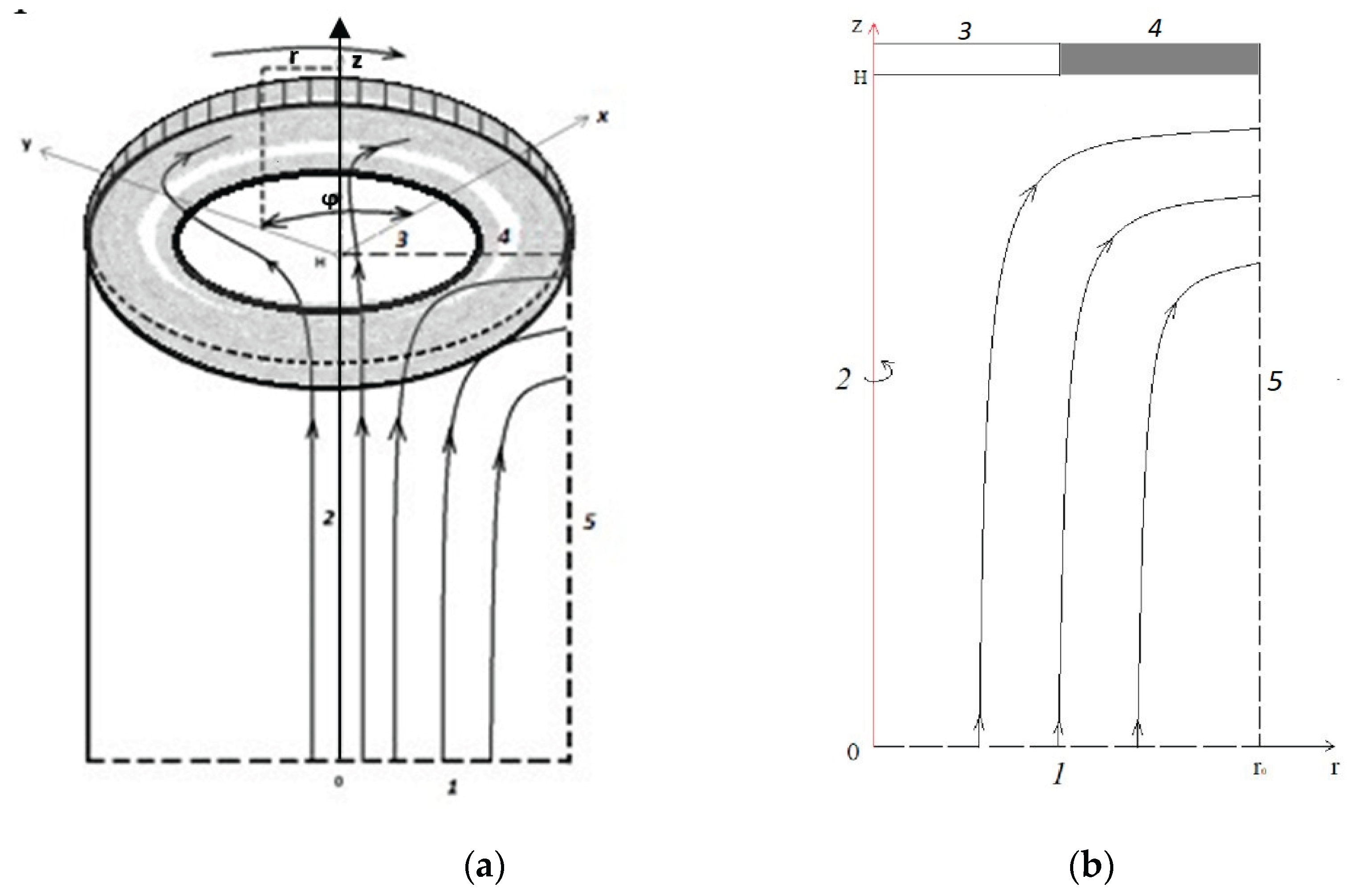
Figure 2.
Graphs at initial concentration : (a) cation concentration when solved by the hybrid method; (b) solution flow lines near the membrane when solved by the hybrid method; (c) cation concentration when solved by the independent finite element method; (d) solution flow lines near the membrane by the independent finite element method.
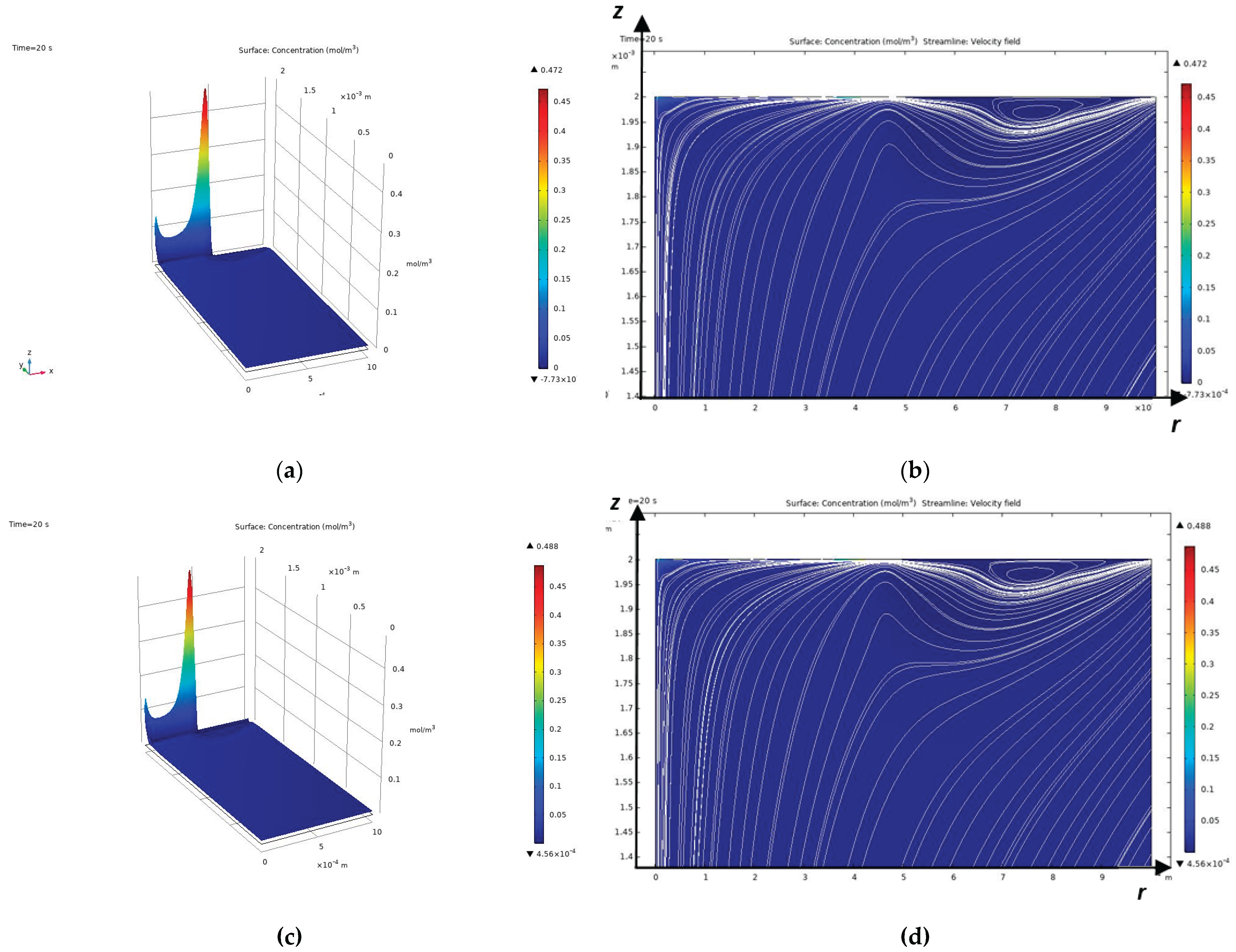
Figure 3.
Graphs at initial concentration : (a) cation concentration when solved by the hybrid method; (b) solution flow lines near the membrane when solved by the hybrid method; (c) cation concentration when solved by the independent finite element method; (d) solution flow lines near the membrane by the independent finite element method.
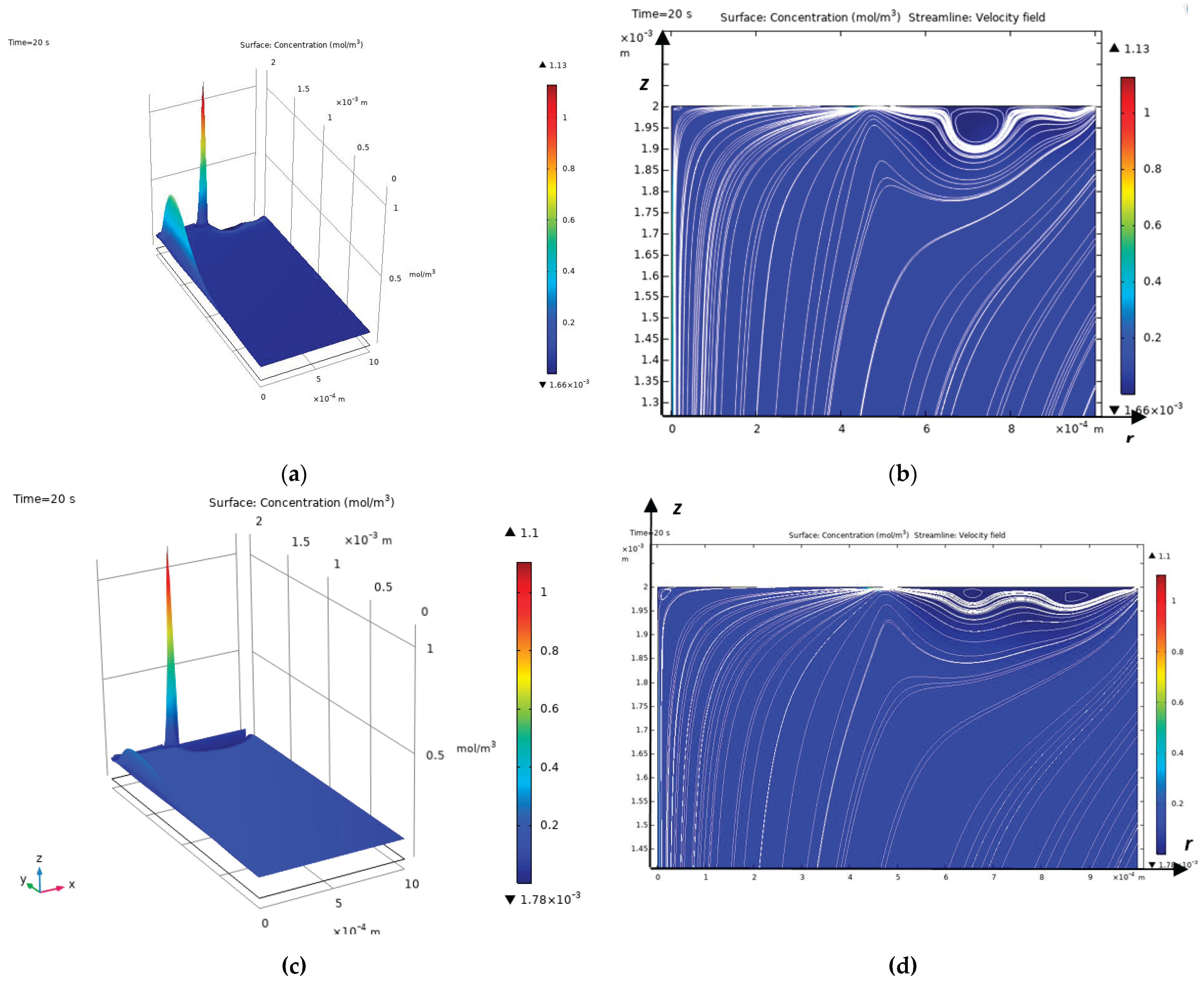
Figure 4.
Solution current lines at a potential jump of 0.1 V: (a) general view; (b) near the membrane.
Figure 4.
Solution current lines at a potential jump of 0.1 V: (a) general view; (b) near the membrane.
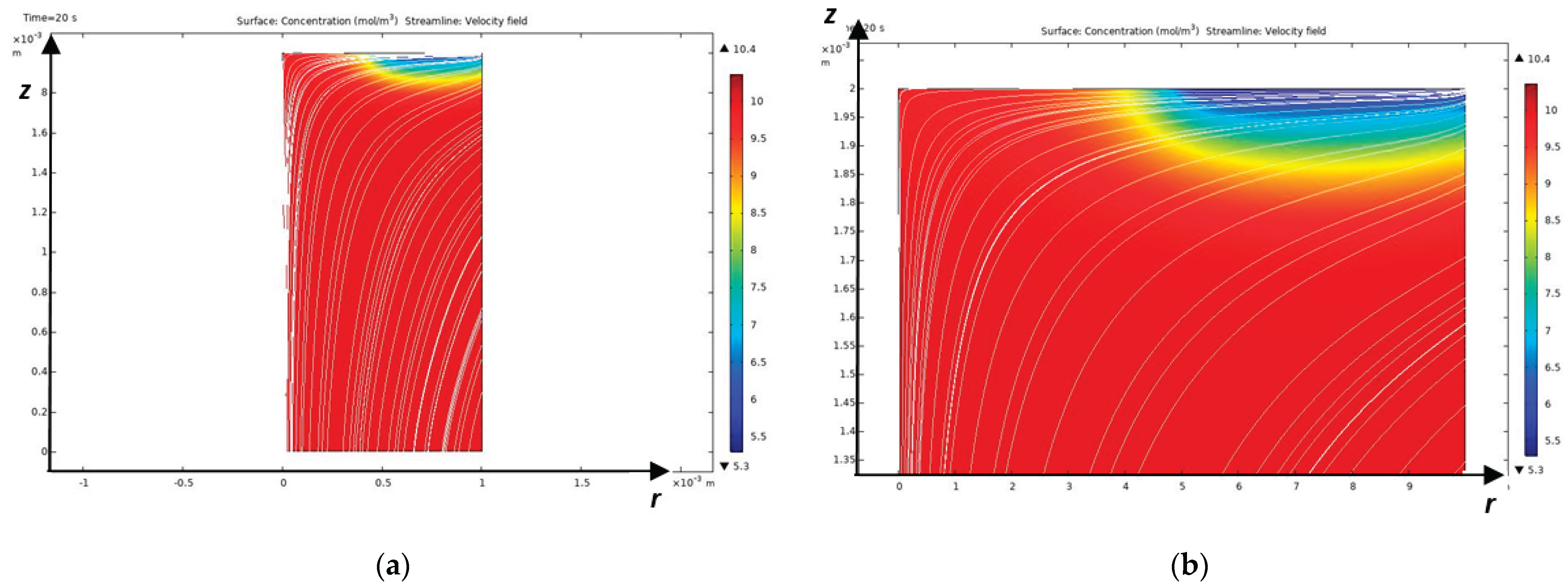
Figure 5.
Graph of solution flow lines near the membrane disk: a) at V and angular velocity rad/s; b) at V and angular velocity rad/s; c) at V and angular velocity rad/s; d) at V and angular velocity rad/s; e) at V and angular velocity rad/s; f) at V and angular velocity rad/s.
Figure 5.
Graph of solution flow lines near the membrane disk: a) at V and angular velocity rad/s; b) at V and angular velocity rad/s; c) at V and angular velocity rad/s; d) at V and angular velocity rad/s; e) at V and angular velocity rad/s; f) at V and angular velocity rad/s.
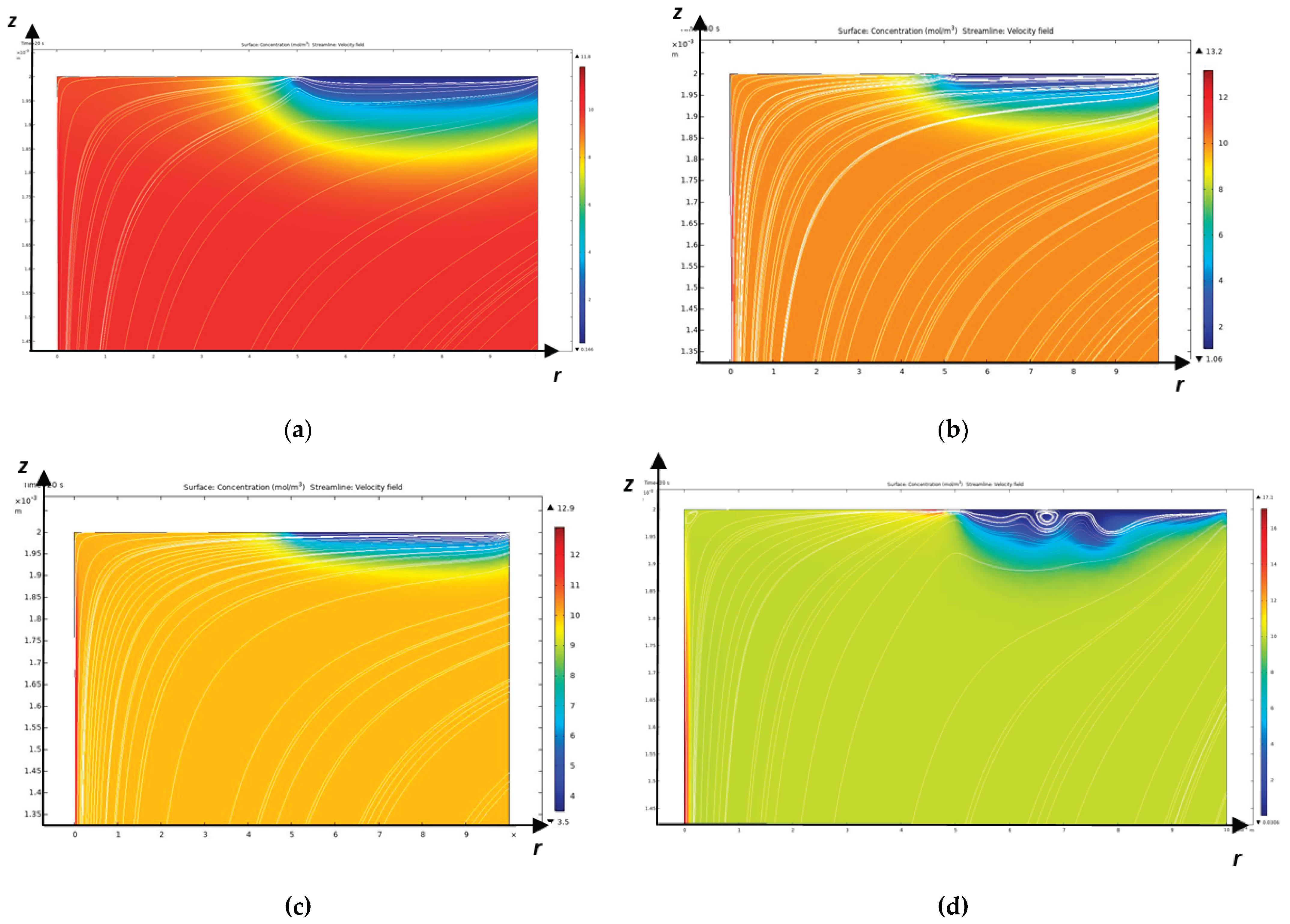
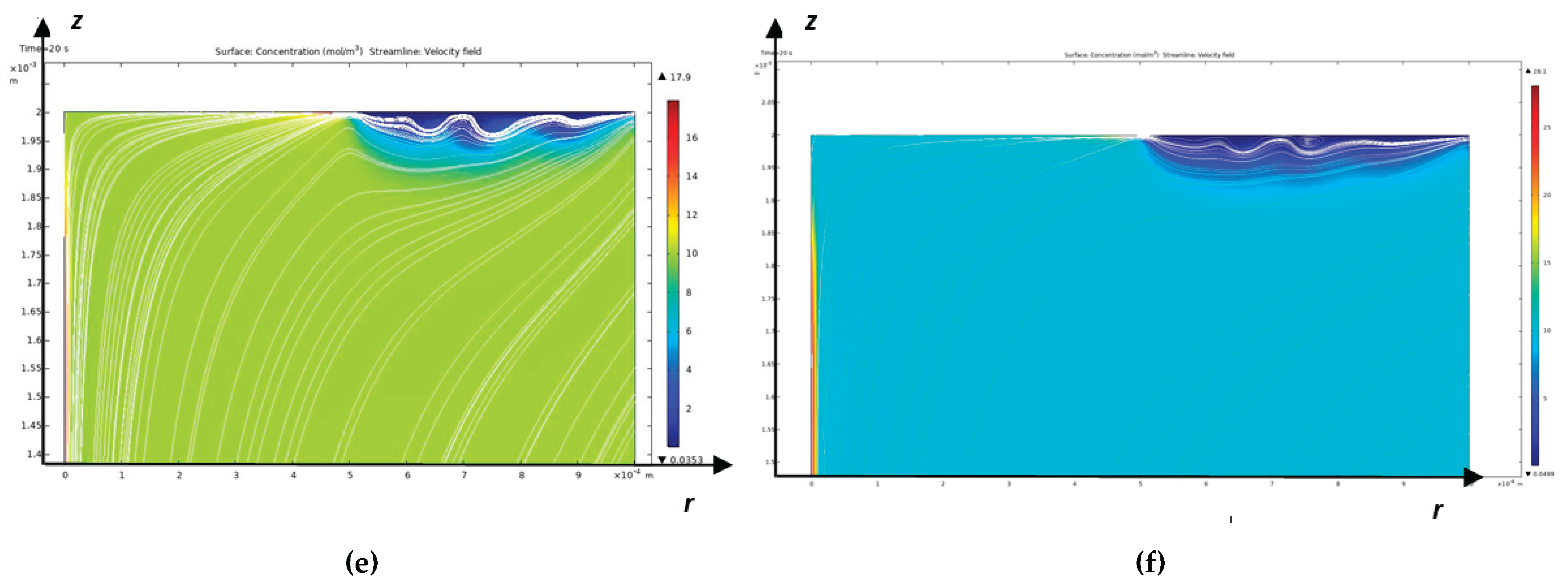
Figure 6.
Graphs of a) cation concentration at ; b) solution flow lines near the membrane at and second; c) solution flow lines near the membrane at and seconds; d) solution flow lines near the membrane at and seconds; e) solution flow lines near the membrane at and seconds.
Figure 6.
Graphs of a) cation concentration at ; b) solution flow lines near the membrane at and second; c) solution flow lines near the membrane at and seconds; d) solution flow lines near the membrane at and seconds; e) solution flow lines near the membrane at and seconds.
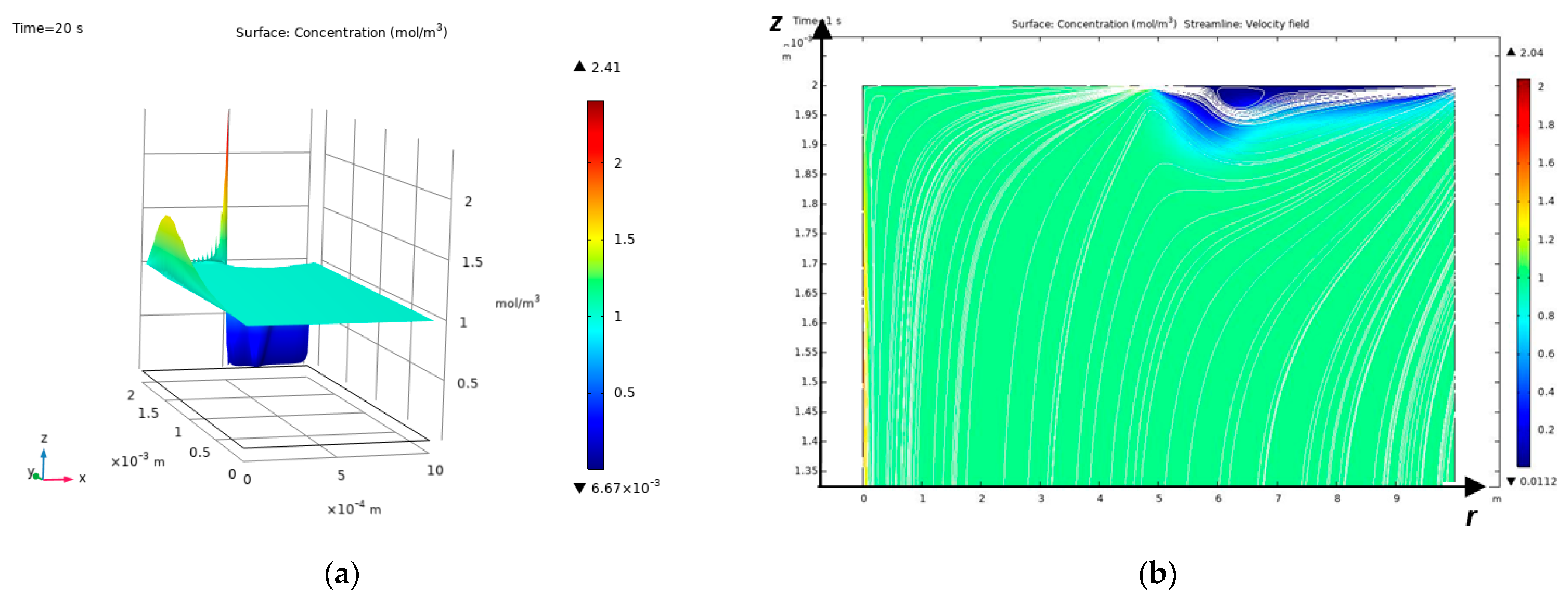

Table 1.
Estimation of the Peclet number at mm.
| 1 | 25 | 100 | |
|---|---|---|---|
| Pe |
Table 2.
Results of Reynolds number estimation at mm.
| ω0 | π/2 | π | 2π | 10π |
|---|---|---|---|---|
| Re | 1.56 | 3.12 | 6.25 | 31.22 |
Table 3.
Parameter estimation .
| C0, mol/m3ω0, rad/s | 0,1 | 1 | 10 | 100 |
|---|---|---|---|---|
| 1 | ||||
| 105 |
Disclaimer/Publisher’s Note: The statements, opinions and data contained in all publications are solely those of the individual author(s) and contributor(s) and not of MDPI and/or the editor(s). MDPI and/or the editor(s) disclaim responsibility for any injury to people or property resulting from any ideas, methods, instructions or products referred to in the content. |
© 2025 by the authors. Licensee MDPI, Basel, Switzerland. This article is an open access article distributed under the terms and conditions of the Creative Commons Attribution (CC BY) license (http://creativecommons.org/licenses/by/4.0/).
Copyright: This open access article is published under a Creative Commons CC BY 4.0 license, which permit the free download, distribution, and reuse, provided that the author and preprint are cited in any reuse.


