
Submitted:
19 May 2025
Posted:
20 May 2025
You are already at the latest version
Abstract
Production involves processes such as raw material extraction, energy consumption, and waste management, which can lead to significant environmental consequences. Therefore, supplier selection based not only on technical performance but also on environmental sustainability criteria has become a fundamental component of eco-friendly manufacturing strategies. Moreover, in the selection of electric vehicle batteries, it is essential to consider customer demands alongside environmental factors. Accordingly, selected suppliers should fulfill company expectations while also reflecting the "voice" of the customer. The objective of this study is to propose an integrated approach for green supplier selection by taking into account various environmental performance requirements and criteria. The proposed approach evaluates battery suppliers with respect to both customer requirements and green criteria. To construct the relational structure, the DEMATEL method was employed to analyze the interrelationships among customer requirements (CRs). Subsequently, the QFD model was used to establish a central relational matrix that captures the degree of correlation between each pair of supplier selection criteria and CRs. Finally, to evaluate and rank alternative suppliers, the Interval Type-2 Fuzzy VIKOR method was applied. A case study was conducted to demonstrate the potential and applicability of the proposed approach. The proposed hybrid model is expected to provide insights for battery suppliers to enhance their competitive advantage by focusing on weaknesses and leveraging strengths through measurable indicators and evaluations. Moreover, the outcomes of the hybrid approach will offer strategic guidance to battery manufacturers for electric vehicles, aiding them in making informed decisions regarding their competitive positioning in the market.

Keywords:
Green supplier selection
; battery selection in electric vehicles
; hybrid decision support system
; DEMATEL-QFD
; interval type-2 fuzzy VIKOR
1. Introduction
Increasing environmental concerns, the depletion risks of fossil fuels, and issues such as global warming have directed the transportation sector towards seeking more sustainable solutions. In this context, Electric Vehicles (EVs) have emerged as an eco-friendly alternative and are rapidly gaining popularity. However, when evaluating the environmental impact of EVs, it is not sufficient to only consider zero exhaust emissions. The production, use, and disposal of batteries which serve as the energy storage systems of these vehicles also represent significant environmental and sustainability criteria. Therefore, the selection of batteries for electric vehicles should not only consider performance and cost but also take into account environmental impacts, the sustainability of raw material sources, recyclability, and life cycle assessments.
The rapid advancements in electric vehicle technologies have made it essential to consider not only technical performance criteria but also environmental sustainability and customer-oriented expectations when selecting batteries. Sustainable green battery selection is a complex decision problem that requires the evaluation of numerous conflicting criteria. In this context, in recent years, Multi-Criteria Decision-Making (MCDM) methods have been frequently used in the literature, with fuzzy logic-based approaches emerging as particularly prominent in situations dominated by uncertainty and complexity. The Decision-Making Trial and Evaluation Laboratory (DEMATEL) method has been utilized as an effective tool to analyze causal relationships and interactions among criteria, providing decision-makers with a systematic perspective. Through this method, not only the importance levels of the criteria but also their interdependencies can be identified. Thus, the DEMATEL method enables the identification of cause-and-effect relationships between customer and environmental criteria, allowing for the distinction between the influencing and influenced criteria in the system. This is a crucial step in identifying which criteria are more critical.
The Quality Function Deployment (QFD) method is regarded as an effective tool for associating customer requirements (CRs) with technical characteristics, offering the advantage of integrating user expectations into technical parameters, especially in the selection of sustainable technological products. Through the integration of DEMATEL and QFD, a bi-directional interaction analysis between stakeholder expectations and technical criteria (green criteria) can be conducted, enabling the creation of more balanced decision models.
The VIKOR method enables the ranking of alternative battery options based on a compromise approach in relation to the ideal solution. Interval Type-2 fuzzy sets, an advanced extension of fuzzy logic, provide higher sensitivity in managing uncertainty in expert opinions and linguistic variables, offering more flexible results compared to classical Type-1 fuzzy sets. This provides a more realistic and adaptable evaluation capability compared to classical fuzzy approaches. In this context, the VIKOR (VlseKriterijumska Optimizacija I Kompromisno Resenje) method, while offering a compromise-based solution for alternative ranking, allows for more reliable outcomes in decision environments characterized by high uncertainty when combined with the interval Type-2 fuzzy extension. Thus, with Interval Type-2 Fuzzy VIKOR (IT2 F-VIKOR), the ranking process becomes more precise and dependable under uncertain conditions. The integration of DEMATEL, QFD, and IT2 F-VIKOR methods will add methodological depth and analytical rigor to the decision-making process. By combining these methods, a holistic, systematic, and reliable battery selection process can be designed, which aligns with both customer-centric and environmental sustainability principles. This approach will not only reduce environmental impacts but also enable more sustainable product and supplier decisions that increase stakeholder satisfaction. Additionally, the development of decision-making approaches for selecting alternatives through integrated methods may be highly specific, as each individual method contains general functions that only provide stable solutions when appropriately integrated.
This study addresses the key factors to be considered in the sustainable "green" battery selection for electric vehicles and compares existing battery technologies in terms of environmental sustainability. The aim is to identify battery alternatives that are less harmful both environmentally and economically, more efficient in terms of resource usage, and compatible with a circular economy. While numerous applications exist in the literature where DEMATEL, QFD, and VIKOR methods are used either individually or in combination, there appears to be a lack of studies focusing on the integrated DEMATEL-QFD-IT2 F-VIKOR model specifically for green battery selection for electric vehicles. Therefore, it is expected that the integrated model proposed in this study will fill the existing gap in the literature and contribute to the development of sustainable decision support systems.
The remainder of this study is structured as follows: The literature review is presented in Section 2. Section 3 introduces the proposed approaches for the five alternatives discussed. Section 4 outlines the steps for applying the proposed integrated approach to green supplier selection. In Section 5, the integrated method proposed is applied to the five alternatives, based on customer and environmental criteria, and the selection and ranking of these alternatives are performed. Section 6 provides an analysis of the application results, while Section 7 concludes with the results and discussions.
2. Literature Review
This section briefly discusses studies related to the use of DEMATEL, QFD, and IT2 F-VIKOR methods in the selection and ranking of alternative suppliers, with a particular focus on their applications in the automotive industry as well as other sectors.
In a study conducted by [1], a decision framework integrating fuzzy DEMATEL, fuzzy QFD, fuzzy TOPSIS, and fuzzy VIKOR methods was proposed for the selection and ranking of five suppliers under 15 criteria in a detergent factory, for the first time in an uncertain environment. In a study by [2], fuzzy DEMATEL and fuzzy QFD methods were used to determine the weights of customer requirements and technical criteria in the product development process for electric vehicles. They also proposed an integrated model using fuzzy VIKOR to scale and evaluate engineering characteristics related to the product development process of electric vehicles. In a study by [3], a hybrid integrated model combining QFD, DEMATEL, and MULTIMOORA methods was used for product design in CNC machine tools. In a study by Zhang et al. (2022), a hybrid decision-making model combining DEMATEL and VIKOR methods for sustainable supplier selection was proposed, and the model was applied in supplier selection evaluation for a company. In a study by [4], strategic part prioritization for quality improvement applications in an automotive factory was conducted. A multi-criteria decision-making approach was used, integrating fuzzy DEMATEL, the anti-entropy weighting method, and fuzzy VIKOR methods. In a study by [5], multi-criteria decision-making methods were used for appropriate supplier selection in the automotive sector. Initially, the DEMATEL approach was applied to reveal the cause-and-effect relationships between the main criteria, followed by the Analytical Network Process (ANP) to calculate the weights of sub-criteria. Finally, alternative suppliers were evaluated using the TOPSIS method, and suppliers with the highest performance index were selected. In a study by [6], a new interval type-2 fuzzy evaluation model utilizing group decision-making analysis for green supplier selection in the automotive sector was proposed. The study was validated with a case study in the battery industry. In the model, the evaluation criteria provided by decision-makers were specified as linguistic terms, which were then converted into interval type-2 fuzzy expressions. The importance of the evaluation criteria was calculated using the interval type-2 fuzzy TOPSIS method, and potential alternatives were ranked using the interval type-2 fuzzy Hamming distance criterion. In a study by [7], a decision support model developed for determining sustainable strategies in the EV adoption process was presented. The approach introduces an interval type-2 fuzzy MEREC-VIKOR approach based on confidence level. The proposed approach allows decision-makers to make evaluations in a more flexible and uncertain environment. The approach used the MEREC (Minimum Removal Effects Criteria) method to determine the importance of criteria in the ranking of strategies, followed by the VIKOR method for the ranking of alternatives. From the literature review (see Table 1), it is observed that many researchers in the past have used a variety of methods and integrated approaches for evaluating and selecting suitable alternatives. However, there is a noticeable lack of studies in the transportation-automotive sector, where customer and environmental criteria are considered in battery selection using the hybrid DEMATEL-QFD-IT2 F-VIKOR method.
3. Preliminaries
This section first presents the concept of type-2 fuzzy sets and the mathematical operations performed within these sets. Subsequently, the steps and definitions of the IT2 FVIKOR method are outlined, followed by the steps and definitions of the DEMATEL method. Finally, the steps and definitions of the QFD method are presented.
3.1. General Type-2 Fuzzy Sets
Type-2 fuzzy sets are a type of fuzzy set developed to better model uncertainty compared to classical or type-1 fuzzy sets. Type-2 fuzzy sets are characterized by membership degrees that are themselves fuzzy and are defined by an upper membership function (UMF) and a lower membership function (LMF).
Definition 1. A Type-2 fuzzy set is defined on the universal set as follows:
Here: : is an element of the universal set .
: The membership degree is the internal variable that varies. : is the range to which the value of belongs for each. : is the second-order membership function that denotes the membership degree of the element and this function defines the type-2 fuzzy set function instead of the type-1 fuzzy set function.
Definition 2. Type-2 fuzzy sets are defined by UMF and LMF. Any type-2 fuzzy set is expressed as follows:
Here: is expressed in terms of the lower and upper membership functions.
Here: represents the UMF
represents the LMF. This definition demonstrates that type-2 fuzzy sets encompass a broader range of uncertainty compared to type-1 fuzzy sets. For this reason, type-2 fuzzy sets can be used to better model uncertainty in fuzzy systems and improve the accuracy of expert opinions.
3.2. Interval Type-2 Fuzzy Sets
Interval Type-2 Fuzzy Sets (IT2 FSs) are a subclass of Type-2 fuzzy sets in which the membership function varies within a specific interval. In these sets, the membership degree of each element is characterized by a lower and upper bound, forming an interval rather than a precise value. This allows for better modeling of uncertainty compared to classical Type-1 fuzzy sets, particularly in situations where information is vague or expert evaluations are imprecise.
Definition 3. Interval Type-2 fuzzy sets are defined as follows:
Here: : denotes an element of the universal set . is the secondary membership function that defines the degree of membership for each element , represented by a bounded interval between a lower and an upper value. These bounds reflect a certain degree of uncertainty.
Definition 4. An interval Type-2 fuzzy set represents each membership value as an interval, and can be expressed as follows:
Here: Upper Membership Function (UMF), represents the highest degree of membership for the element .
Lower Membership Function (LMF), represents the lowest degree of membership for the element .
The lower and upper membership functions represent the fuzzy value range assigned to an element, which is particularly useful for modeling more complex and uncertain systems.
3.3. Arithmetic Operations in Type-2 Fuzzy Sets
Definition 5. Addition Operation: In type-2 fuzzy sets, the addition operation is performed between the lower and upper membership functions of each set.
If and are type-2 fuzzy sets, the membership function of the set is calculated as follows:
Here: and are the lower and upper membership functions of the set . and are the lower and upper membership functions of the set .
Definition 6. Subtraction Operation: The subtraction operation allows for finding the difference between two Type-2 fuzzy sets. This operation is performed between the lower and upper membership functions of both sets.
If we are working with Type-2 fuzzy sets and the membership function of set is calculated as follows:
Here: and are the lower and upper membership functions of set . ve are the lower and upper membership functions of set .
Definition 7. Multiplication Operation: The multiplication operation is performed between the lower and upper membership functions of Type-2 fuzzy sets. This operation yields the result obtained by multiplying the membership degrees of the two Type-2 fuzzy sets.
If we are working with Type-2 fuzzy sets and , the membership function of set is calculated as follows:
Here: and are the lower and upper membership functions of set . and are the lower and upper membership functions of set .
Definition 8. Division operation. The division operation is also performed between the membership functions of two Type-2 fuzzy sets, where the membership function of one set is divided by the membership function of the other set.
If we are working with Type-2 fuzzy sets and , the membership function of set is calculated as follows:
Here: and are the lower and upper membership functions of set . and are the lower and upper membership functions of set .
Definition 9. Multiplying a Type-2 fuzzy set by a constant . The operation of multiplying a Type-2 fuzzy set by a constant is performed as follows:
Similarly, the membership function of set is calculated as follows:
Here: a constant number (usually a positive real number).
and are the lower and upper membership functions of set. is the new type-2 fuzzy set multiplied by the constant .
Definition 10. Triangular type-2 fuzzy sets: Triangular type-2 fuzzy sets are typically defined by their lower and upper membership functions. Although they have a triangular shape, similar to type-1 fuzzy sets, they contain two membership functions: UMF and LMF. A triangular type-2 fuzzy set is defined by the following parameters:
UMF: A triangular fuzzy number is denoted as ).
LMF: It is typically defined as a smaller triangular fuzzy number within the UMF, for example, denoted as ). In a type-2 triangular fuzzy set, the horizontal axis represents the variable value, and the vertical axis represents the membership degree value. A type-2 triangular fuzzy set is shown in Figure 1.
3.4. Interval Type-2 Fuzzy VIKOR Method (IT2 F-VIKOR)
This section will discuss the steps involved in the IT2 F-VIKOR method.
Step 1: First, the number of decision makers, alternatives, and criteria are determined.
Step 2: Determining Fuzzy Data. In this step, decision makers evaluate each alternative for each criterion using interval type-2 fuzzy numbers. Interval type-2 fuzzy numbers are typically expressed with lower and upper bounds that are defined within specific intervals. The alternatives (A1, A2 ,..., An) and criteria (C1, C2, ..., Cm) are determined. The decision matrix is created as follows:
Step 3: Calculation of the ideal (positive) and anti-ideal (negative) solutions. At this stage, the ideal solution () and the anti-ideal solution () values are calculated for each criterion. The ideal solution (): It takes the best (maximum) values for each criterion. The anti-ideal solution (): It takes the worst (minimum) values for each criterion. The ideal and anti-ideal solution values are calculated as shown in Eq. (12) and (13) below:
Here; for Type-2 fuzzy numbers, the upper and lower membership functions are normalized separately.
Step 4: Fuzzy data normalization. In this step, the fuzzy data for each alternative and criterion are typically normalized to a specific range. Normalization converts the value of each criterion to a range between 0 and 1, ensuring comparability among criteria. The formulas for normalization are given in Eq. (14) and (15) as follows:
Here;
, It is a measure of the total difference (the overall distance of the alternative in relation to all criteria).
, It is the maximum criterion difference (the distance of the alternative in the worst criterion).
, j. is the weight of the criterion..
Here; For Type-2 fuzzy numbers, the upper and lower membership functions are normalized separately.
Step 5: The calculation of the fuzzy VIKOR scores. The fuzzy VIKOR score is calculated based on the distances of each alternative from the ideal and anti-ideal solutions. This computation incorporates the decision-maker’s compromise parameter , which reflects the balance between the proximity to the ideal solution and the remoteness from the anti-ideal solution. The VIKOR score is calculated as shown in Eq. (16) below.
Here;
: The total disadvantage of the alternative
: The worst criterion performance of the alternative
: , : , : , :
: The compromise coefficient (usually set to 0.5).
Step 6: Defuzzification of the Calculated Fuzzy VIKOR Scores. In this step, the fuzzy VIKOR scores computed in step 5 are defuzzified to obtain crisp values. The defuzzification of the Type-2 fuzzy VIKOR scores will be carried out using the average Type-1 fuzzy approach. This method involves a two-step defuzzification process.
-
Transformation of Upper and Lower Membership Functions into Type-1 Fuzzy Sets: Here, to obtain a Type-1 fuzzy set, the average of the upper and lower membership functions is calculated.Here; represents the value of the upper membership function, and represents the value of the lower membership function.As a result of this process, our type-2 fuzzy set is transformed into a type-1 fuzzy set.
- Defuzzification: Here, the Weighted Average (Centroid) Method is applied to defuzzify the type-1 fuzzy set: This significantly simplifies the computation required to find the center of a two-dimensional shape, thus enhancing the efficiency of the defuzzification process [13].
Thus, using Eq. (17) and (18), the type-2 fuzzy values calculated in Step 5 are defuzzified and converted into crisp values.
Step 7: Ranking of Alternatives. In Step 6, alternatives are ranked based on the VIKOR scores (Qi) calculated. The alternative with the smallest VIKOR score is considered the best solution.
Here; Two conditions are checked for the Qi value:
Condition 1 (Acceptable Advantage):
Here; A1: Represents the best alternative, A2: Represents the second best alternative, and m: Represents the total number of alternatives considered.
Condition 2 (Acceptable Stability): The best alternative must be ranked first in both the and rankings. If these conditions are not met, a compromise can be made to select the best alternative.
3.5. DEMATEL Method (The Decision Making Trial and Evaluation Laboratory Method)
The DEMATEL method was developed between 1972 and 1976 by the Battelle Memorial Institute in Geneva, under the Science and Human Relations Program, for solving complex and interrelated problem groups [14]. The DEMATEL method consists of seven consecutive steps. The solution is achieved with the effect-cause graph diagram obtained at the end of Step 5.
Step 1: The creation of the direct relationship matrix (A):
To create the direct relationship matrix (A), a five-level binary comparison scale is used. The levels are represented as 0 (Ineffective), 1 (Low Impact), 2 (Moderate Impact), 3 (High Impact), and 4 (Very High Impact). The relationships between criteria are determined by an expert group using the binary comparison scale [15]. As a result of the comparisons, the direct relationship matrix (A) is obtained. A sample A matrix is shown in Eq. (20).
Step 2: The creation of the normalized direct-relation matrix (X):
After the creation of the direct-relation matrix (A), the normalized matrix (X) is obtained using Eq. (21). Each element in the X matrix is between 0 and 1.
Here;
Step 3: Calculation of the total relation matrix (T):
After obtaining the normalized direct-relation matrix, the total relation matrix is derived using Eq. (23). In this equation, the identity matrix (I) is denoted.
Step 4: Determination of the row and column sums of the T matrix:
In the total relation matrix (T), the sums of the rows and columns are obtained using Eq. (24) and (25), and these are represented by the vectors D and R, respectively.
Step 5: Adjustment of the threshold value (α):
To obtain an appropriate cause-effect graph, decision-makers need to adjust a threshold value for the impact level. Elements with impact values greater than the threshold in the T matrix are selected and transformed into a cause-effect graph diagram. The threshold value is determined by the decision maker or experts. The value of is calculated using Eq. (26). Here, N represents the total number of elements in the T matrix.
Step 6: Development of a Causal Diagram:
A causal diagram is a classification of the degree of each criterion. It shows the criteria that can easily be classified as passive or active. The influence-diagram is obtained by plotting the points (D+R, D-R) on a coordinate plane, where the horizontal axis represents D+R and the vertical axis represents D-R.
Step 7: Calculation of criteria weights:
The criteria weights are calculated by normalizing the prominence vector (Dk + Rk), ensuring that the sum of the normalized weights equals 1.
3.6. QFD Model
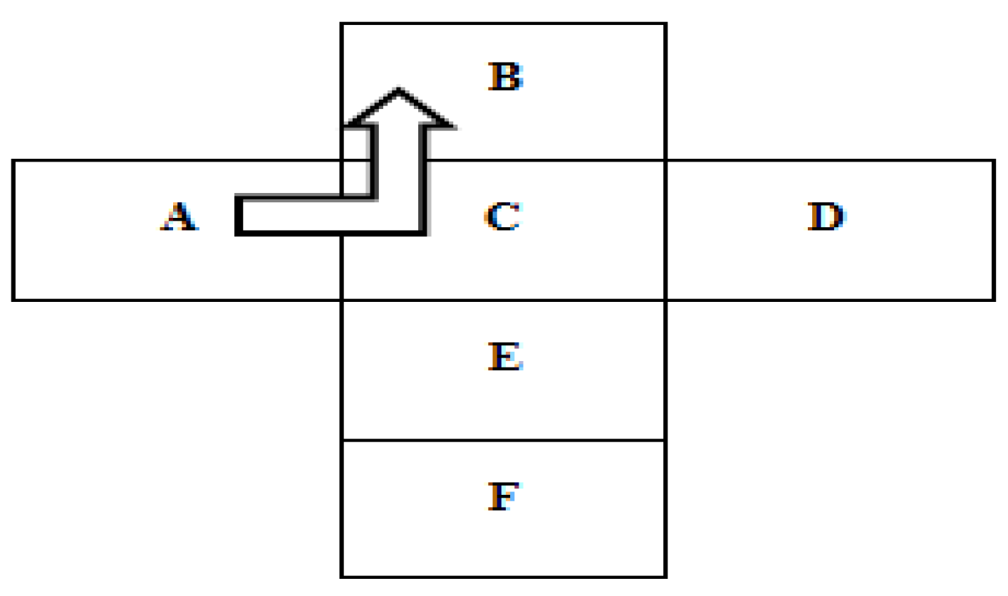
In a general QFD model, the following elements are incorporated into the House of Quality (HoQ), as illustrated in Figure 2. Here;
A: The matrix of WHAT’s, B: The matrix of HOW’s, C: The relationship matrix between WHAT’s and HOW’s, D: The relative importance or weights of the WHAT’s, E: The relationship among the HOW’s, F: It represents the weights of the HOW’s.
The general QFD model is shown in Figure 2 below.
Figure 2.
General QFD model.
The general steps in applying the QFD model are as follows:
Step 1: The definition of the WHAT’s is made.
Step 2: The definition of the HOW’s is made. The supplier selection criteria are specified as HOW’s in the HoQ and placed in the area marked ‘B’ in Figure 2.
Step 3: The development of the HOW’s matrix (E) showing the internal dependencies among the HOW’s.
Step 4: Assigning priority weights to customer requirements: A binary comparison scale consisting of 5 levels is used to assign priority values to customer requirements. The levels are defined as 1 (Not important), 2 (Important), 3 (Very important), 4 (Much more important), and 5 (Most important).
Step 5: The development of the relationship matrix (C) or HoQ by evaluating the degree of impact between the WHAT’s and HOW’s, using an appropriate scale to express how much each WHAT’s affects the HOW’s. Here, a four-point scale of 1, 3, 6, and 9 is used, addressing weak, medium, strong, and very strong relationships, respectively.
Step 6: After the HoQ matrix is developed, the overall priorities of the supplier selection criteria or HOW’s are calculated, showing the synthesized importance of the supplier selection criteria.
In QFD, the output of each stage (HOW’s) is transformed into the inputs of the next stage (new WHAT’s). The advantages of implementing the QFD model include higher customer satisfaction, shorter delivery times, better flexibility, promotion of quality, reduced time to market, and information protection, among others [16].
4. A Combined Selection Method for Green Supplier Selection
The proposed hybrid approach will provide the following contributions to the literature. The first contribution is the integration of customer requirements and green supplier selection criteria. The second contribution is the presentation of DEMATEL, QFD, and IT2 F-VIKOR methods as an integrated framework. The DEMATEL-QFD component of the proposed hybrid method provides a practical and effective approach for performing customer-oriented criteria weighting in situations where customer satisfaction is directly involved in the decision-making process. The IT2 F-VIKOR method, on the other hand, has been applied to evaluate and rank suppliers based on each selection criterion. The complete approach, which is being proposed for the first time, is summarized below in a four-stage structure:
4.1. Stage I: Identification of Customer, Green Supplier Selection Requirements, and Alternatives
In this stage, a two-person expert committee was formed. Then, based on the literature review and the characteristics of the analyzed supplier companies, CRs and supplier selection criteria related to sustainable green factors were determined in collaboration with the expert committee. The customer criteria determined in this stage represent the answers to the "What" questions of the problem at hand. The green supplier selection criteria include all the criteria that need to be considered for ranking the candidate suppliers, i.e., all the CRs to be fulfilled, and these criteria represent the answers to the "HOW" questions of QFD in the addressed problem. Based on the literature review and the views and recommendations of the expert committee, the CRs, green supplier criteria, and the evaluated alternatives along with their explanations are provided in Table 2 and Table 3 below.
4.2. Stage II: Weighting of Customer and Green Supplier Selection Criteria
In this stage, the DEMATEL method is used to establish the causal and perceptual relationship between the CRs and the green supplier selection criteria, assigning overall weights. Subsequently, the normalized values of the CRs, obtained through the DEMATEL method in the previous stage, are considered as the CRs' weights to be used later in the QFD-based analysis. These weights are then used to weight the green supplier selection criteria in the QFD. The QFD model is defined as follows by [17]: QFD transformations are typically represented by a matrix known as the House of Quality (HoQ). This matrix expresses the relationship between the CRs (WHAT’s) and the green supplier selection criteria (HOW’s), containing the following elements: Here; A) The matrix of WHAT’s, B) The importance (weights) of the WHAT’s, C) The matrix of HOW’s (green supplier selection criteria), D) The relationship matrix between WHAT’s and HOW’s, E) The matrix to relate HOW's, F) the relative importance or weights of HOW's (the weights of green supplier selection criteria) and G) It represents the competitive evaluation matrix [17]. The working principle of QFD is provided in Figure 3.
4.3. Stage III: Weighting of Suppliers According to Each Green Supplier Selection Criterion
In this stage, the expert committee evaluates the alternatives according to each green supplier selection criterion in order to determine the performance score of the candidate suppliers based on green criteria. For this, the expert committee will assess each candidate supplier separately according to the green supplier selection criteria using interval type-2 triangular fuzzy numbers.
4.4. Stage IV: Ranking Alternatives Using the IT2 F-VIKOR Method
In this phase, the IT2 F-VIKOR method is applied to rank the suppliers. To implement this method, both the weights of all green supplier selection criteria from the second phase and the priority values of each candidate supplier according to each green supplier selection criterion obtained in the third phase will be used to evaluate and rank the candidate suppliers.
5. Application of the Proposed Method
In this section, the steps of the DEMATEL-QFD-IT2 F-VIKOR hybrid method are applied to a supplier selection problem. The application process consists of three stages: In the first stage, the criteria and alternatives related to the problem are defined. Then, a committee consisting of experts is formed, and the evaluation process begins. During this stage, the criteria and alternatives are assessed by the experts in accordance with the purpose of the problem. In the third stage, based on the experts' evaluations, the method(s) applied result in the selection and ranking of the alternatives.
Based on expert opinions and a literature review, 5 CRs criteria, 5 sustainable green supplier criteria, and 5 alternatives have been identified. In this study, all 5 CRs defined are considered vital, and therefore, identifying the most important requirement of the evaluation system and measuring the relationships between them is essential. For this reason, the DEMATEL method was used to measure the causal relationships among the CRs. As explained in the DEMATEL steps in Section 3.5, integer scale is used to determine the relationships between different CRs. After the relationships are measured, the initial direct relationship matrix (A) is created, as shown in Table 4. Matrix A is a 5x5 matrix obtained through bidirectional comparisons, representing the effects and directions between the CRs.
The normalized direct-relation matrix (X) is calculated from the A matrix in Table 4, as presented in Table 5.
Now, the row and column totals, represented by the D and R vectors, are calculated as shown in Table 7.
Using Table 7, the total and net impact values (D+R) and (D-R) for each CR are calculated as shown in Table 8.
The values of (D+R) and (D-R) in Table 8 represent the degree of total impact levels and, respectively, the degree of net impact levels. Positive values here indicate that they will affect other requirements more. Table 8 shows that the EFR customer demand has the highest impact level, followed by the LR demand. The causal diagram of DEMATEL for CRs.
Looking at the causal diagram in Figure 4, it can be seen that the CRs are visually divided into cause and effect groups. The causal group is formed by S and EFR, while the effect group is formed by LR, FCT, and LC. It is credible that the requirements of S and EFR are the main driving factors for LR, FCT, and LC. Among these five CRs, EFR is considered the most important value because it has the maximum D + R value and thus has the strongest relationship intensity with the others. Additionally, EFR is also the most convincing factor due to its highest D-R value. Therefore, EFR plays a significant role in the supplier evaluation problem and has the greatest impact on the others. On the other hand, LC, with the lowest (D-R) value, is the customer demand most affected by the other factors.
The threshold value (α) is calculated by taking the average of the elements in the T matrix using Eq. (26). Here, the α value is calculated as 0.3704. The tij values in Table 6 represent the relationship between two CRs, and the relationships are compared with the cause-effect values tij* value. For example, since (0.3752) > α (0.3704), the arrow in the diagram is drawn from LR to S as shown in Figure 5. The contextual relationships among the CRs are presented in Figure 5.
The weights of the CRs are calculated by normalizing the (D + R) values presented in Table 8 and are shown in Table 9. As can be seen from Table 9, EFR has the highest weight and the greatest impact among the other factors.
As shown in Table 9, among the CRs, the highest weight is assigned to the EFR criterion, indicating that it has the greatest overall impact on the system.
Following the calculation of the weights of the CRs, and in accordance with the QFD process (see Section 3.6), a central relationship matrix is constructed to illustrate the interactions and correlations between each pair of CRs and the green supplier selection criteria. This relationship matrix, presented in Table 10, is developed by the decision-making team based on the available data regarding green suppliers. Essentially, this step addresses how the CRs and the green supplier selection criteria interact and influence each other, based on expert evaluations. As shown in Table 10, values are assigned within the matrix to represent how well each green supplier selection criterion satisfies each CR. Using both the weights of the CRs and the expert assessments, the weights of each green supplier selection criterion are calculated. The normalized weights of all green supplier selection criteria are obtained and presented in Table 10. It is clearly observed that the EELI criterion emerges as the most critical green supplier evaluation criterion among the listed criteria.
After calculating the weights of the green supplier selection criteria using the QFD model, the IT2 F-VIKOR method will be employed to evaluate the alternatives based on each green supplier evaluation criterion.
5.1. Ranking of Alternatives Using IT2 VIKOR
In this section, the applicability of the IT2 FVIKOR method to the battery selection problem in electric vehicles based on green criteria is demonstrated step by step. The objective of the decision problem is to select and rank five alternatives (A1, A2, A3, A4, A5) (see Table 3) under five green criteria (CF, WMRR, TCMU, GEU, EELI) (see Table 2), which are defined by the expert committee. Here;
CF: Carbon footprint (CO₂ Emissions) (g CO2/kWh) (to be minimized) (1-10 points)
WMRR: Waste management and recycling rate (to be maximized) (1-10 points)
TCMU: Use of toxic and critical materials (Yıl) (to be minimized) (1-10 points)
GEU: Use of green energy (to be maximized) (1-10 points)
EELI: Energy efficiency and lifetime impact (to be maximized) (1-10 points)
Here; 1: epresents the lowest------ 10: Represents the highest score.
The green supplier criteria weights obtained from the DEMATEL-QFD hybrid method were presented in Table 10. Now, let us explain step by step the application of the IT2 F-VIKOR method to the alternative selection problem at hand:
Step 1: The decision matrix creation. In this step, the decision matrix for evaluating the five alternatives according to the criteria, formed by a two-person expert committee, is provided in Table 11. Interval type-2 triangular fuzzy numbers were used to construct the decision matrix.
Step 2: Calculation of Ideal (Positive) and Anti-Ideal (Negative) Solutions. In this step, the ideal solution and the anti-ideal solution for each criterion are calculated. The ideal solution is calculated using Eq. (12), and the anti-ideal solution is calculated using Eq. (13). The calculated values are presented in Table 12.
Step 3: The calculation of normalized fuzzy values. In this step, fuzzy and values, which represent the deviation measures for each alternative, will be calculated using Eq. (14) and (15). Since the detailed calculations are quite lengthy, only the calculation process for alternative A1 will be performed. The fuzzy and values for the other alternatives are calculated similarly. Now, let's calculate the preliminary values for alternative A1 based on the fuzzy and values.
For alternative A1, the upper membership values for CF (the criterion to be minimized) are as follows:
Now, if we multiply the value calculated above by the weight (see Table 10):
For alternative A1, the lower membership values for CF (the criterion to be minimized) are as follows:
it is calculated as.
Now, if we multiply the value calculated above by the weight (see Table 10):
it is calculated as.
Thus, the interval type-2 fuzzy membership value calculated for CF of alternative A1 is found to be .
For alternative A1, the upper membership function for WMRR (criterion to be maximized) is as follows:
Now, if we multiply the value calculated above by the weight (see Table 10);
it is calculated as.
For the A1 alternative, the lower membership function for WMRR (the criterion to be maximized) is calculated as follows:
it is calculated as.
Now, if we multiply the value calculated above by the weight (see Table 10);
it is calculated as.
Thus, the interval type-2 fuzzy membership value calculated for WMRR of the A1 alternative is computed as . Similarly, the calculated interval type-2 fuzzy upper and lower membership values for the TCMU, GEU, and EELI criteria are provided below:
The calculated interval type-2 fuzzy membership value for the TCMU criterion: The calculated interval type-2 fuzzy membership value for the GEU criterion: (0.1070, 0.1051, 0.1027;1,1)(0.1107, 0.1051, 0.0988;)
The calculated interval type-2 fuzzy membership value for the EELI criterion: (0.1525, 0.1663, 0.1829;1,1)(0.1630, 0.1829, 0.1700;)
Similarly, the preliminary values for the fuzzy and values of the remaining alternatives have been calculated through similar procedures as described above, and the calculated preliminary interval type-2 fuzzy membership values for and are presented in Table 13.
Now, based on Table 13, the final and values for each alternative have been calculated (according to Eq. (14) and (15)). The calculated final and values are presented in Table 14.
Adım 4: Calculation of the Fuzzy VIKOR Index (). In this step, the fuzzy VIKOR score () for each alternative will be calculated using Eq. (16). As an example, the fuzzy VIKOR index value for alternative A1 has been calculated. Similar operations are performed for the other alternatives. The fuzzy VIKOR index values for all alternatives are presented in Table 15. Now, let's calculate the fuzzy VIKOR index value () for alternative A1:
The formula used to calculate the final decision score in the interval type-2 fuzzy VIKOR method is presented below.
Here;
: The total disadvantage of the alternative, : the worst criterion performance of the alternative
: , : , : , : , : the compromise coefficient (commonly taken as 0.5)
Based on Table 14, the best and worst values for each alternative and criterion are provided below:
,
,
(0.9584, 0.9610, 0.9503;1,1)(0.9559, 0.9610, 0.9684;)
,
Calculation of for Alternative A1:
The first term; Now, let us multiply the calculated first term by the weight coefficient :
The second term; Now, let us multiply the calculated second term by the weight coefficient :
As a result, the final value for the A1 alternative is calculated as:
. Similar calculations are carried out for the remaining alternatives in the same manner, and the computed fuzzy VIKOR index () values are presented in Table 15.
Step 5: The defuzzification of the calculated fuzzy VIKOR scores. In this step, the IT2 F-VIKOR scores calculated from Table 15 will be converted into crisp values using Eq. (17) and (18). Since the defuzzification process for all alternatives will be lengthy, we will demonstrate the defuzzification process only for the A1 alternative. Similar processes will be applied to the other alternatives as well. Now, let’s go step by step through the defuzzification process for the A1 alternative:
Using Eq. (17), the defuzzified crisp value for A1 is calculated using the formula , and using Eq. (18), the final defuzzified crisp value for A1 is computed as follows:
The defuzzified value is calculated as
Similar operations have been performed for alternatives A2, A3, A4, and A5, and the defuzzified values for all alternatives are presented in Table 16.
Here; According to Eq. (19), in the VIKOR method, the minimum acceptable advantage value is used to determine whether one alternative is significantly better than the others.
Since the acceptable advantage condition is not provided with the value, a compromise (acceptable stability condition) selection path should be followed instead of determining a single best alternative. For this purpose, the and values will be examined. Because, in the compromise selection process, the alternatives should be analyzed not only based on their values but also in terms of their (group utility) and (individual regret) values. In this context, if the alternative with the best Qi value (i.e., Alternative A3) also ranks first in both and , it can be directly selected as the most appropriate alternative. If different alternatives outperform others across different criteria, a compromise decision becomes necessary. According to Table 16, Alternative A3 is identified as the best option, followed by Alternative A1 as the second-best. According to Table 14, the and values of alternative A3 are better than those of alternative A1. Similarly, Table 14 also shows that alternative A3 has the best Si and Ri values among all alternatives, indicating the lowest values. Since A3 ranks first in both the (group utility) and (individual regret) criteria, the acceptable stability condition is satisfied. Alternative A1, on the other hand, should be considered as the second-best option due to the insufficient advantage gap.
6. Analysis of Result
This study addresses the battery selection problem for firms engaged in electric vehicle (EV) manufacturing. For the selection of alternative batteries, an expert committee consisting of two specialists in the field was initially formed. Based on the recommendations of the established expert committee and findings from the literature review, five criteria were selected for both customer requirements and green supplier selection, along with five alternative suppliers. The five candidate alternatives identified were evaluated against the determined customer and green supplier selection criteria using the novel hybrid DEMATEL-QFD-IT2 F-VIKOR approach proposed in this study. The DEMATEL method was initially employed to identify critical requirements among the five predetermined CRs and to measure their interrelationships. According to the results of the DEMATEL analysis applied to the CRs, the criterion of being environmentally friendly and recyclable has been identified as the most influential factor in battery selection. Subsequently, among the CRs, the criterion of long driving range was identified as having the second highest level of influence. The other criteria with the highest levels of influence among the CRs were found to be, in order, low cost, safety, and fast charging time. When examining the causal relationships among the CRs, it was observed that the criteria of being environmentally friendly and recyclable, along with safety, were the most influential causal factors affecting the other criteria (see Table 8). The criteria of long driving range, fast charging time, and low cost were identified as the most affected by other criteria (see Table 8). Additionally, according to Table 8, the criterion of being environmentally friendly and recyclable plays a significant role in the evaluation of alternatives and exerts the greatest influence on the other CRs. Similarly, the low-cost criterion was found to be the most affected customer requirement among all CRs.
In the proposed hybrid model, the QFD (Quality Function Deployment) approach was employed to demonstrate the effects and relationships between each pair of CRs and the green supplier selection criteria. Here; the relationship matrix between CRs and green supplier selection criteria was developed by the decision-making team based on available information regarding green suppliers (see Table 10). As a result of the relationship matrix constructed by the expert committee, the calculated weight values for the green supplier criteria are presented in Table 10 and also illustrated graphically in Figure 6. Among the green supplier selection criteria, the EELI criterion was identified as the most important evaluation criterion (see Table 10 or Figure 6).
In the proposed hybrid model, following the calculation of the weights of customer requirements and green supplier selection criteria based on the DEMATEL-QFD methods, the Interval Type-2 Fuzzy VIKOR (IT2 F-VIKOR) method was employed to select and rank the five considered alternatives.
In this method, the five considered alternatives were primarily evaluated based on the previously identified green supplier selection criteria: CF, WMRR, TCMU, GEU, and EELI. Using the IT2 F-VIKOR method, the ranking values of the five considered alternatives were calculated as follows: A1 = 0.1817, A2 = 0.2427, A3 = 0.0000, A4 = 1.0000 and A5 = 0.4183. Accordingly, the ranking performance values calculated for the alternatives, considering customer requirements and green supplier selection criteria, are presented in Figure 7. The performance rankings of the alternatives within the scope of this study are also provided in Table 17.
The ranking performance scores of the alternatives, calculated using the proposed hybrid DEMATEL-QFD-IT2 F-VIKOR methodology, are presented in Table 17.
According to Table 17, when both customer requirements and green supplier selection criteria are considered together, it is acceptable for vehicle manufacturers or battery suppliers selecting batteries for electric vehicles to prioritize Alternative A3. Likewise, it would be appropriate for the same firms or suppliers to consider Alternative A1 as the second-best option. In contrast, based on customer requirements and green supplier criteria, Alternative A4 appears to be the least preferred choice for battery selection in electric vehicles.
7. Conclusion and Discussion
With the radical transformations occurring in environmental issues, public pressure and environmental logistics have become increasingly significant in the management of environmental and social aspects of business operations. In the context of electric vehicles, battery selection plays a critical role in terms of performance, safety, and environmental sustainability. In this process, both customer requirements and supplier criteria -particularly those related to green suppliers- must be taken into account. These criteria contribute not only to regulatory compliance but also to the sustainability goals and corporate social responsibility strategies of firms. Therefore, for electric vehicle manufacturers, the appropriate selection of batteries is not solely based on technical and economic performance, but also requires a holistic approach that minimizes environmental impacts and creates long-term value. Consequently, the use of integrated decision-making models that balance customer expectations with green supplier criteria has become essential.
A review of the literature reveals that many researchers have applied fuzzy MCDM methods to supplier selection problems in comparison with traditional MCDM methods. The findings indicate that fuzzy MCDM approaches generally provide more effective ranking outcomes than their conventional counterparts. Furthermore, the integration of fuzzy numbers with decision-making methods has been widely addressed by numerous scholars. However, combining fuzzy numbers with type-2 fuzzy sets offers greater flexibility and accuracy in complex decision-making processes. In this study, the VIKOR method -one of the prominent MCDM techniques- was integrated with interval type-2 fuzzy sets. The main advantage of the proposed method lies in incorporating expert knowledge into the traditional MCDM method, VIKOR, and successfully integrating it with type-2 fuzzy numbers for application in the alternative selection problem. While many studies have addressed the impact of customer satisfaction indices and engineering characteristics on the supplier selection process, to the best of our knowledge, none have systematically examined how these variables interact with each other. This indicates a significant gap, particularly in the systematic analysis of sustainable green suppliers [18]. To fill this gap, it is essential to connect all organizational elements that contribute to performance measurement, including the green structures and infrastructures of sustainable green suppliers [19]. With the hybrid method proposed in this study, we aim to close both of these gaps by providing a systematic analysis of the interdependencies between customer variables and green supplier selection criteria.
For the reasons mentioned above, in this study, we proposed a hybrid method for battery selection in electric vehicles, which considers both customer demands and sustainable green supplier selection criteria. Therefore, the primary aim of this study is to address the problem of evaluating and ranking green suppliers using an integrated formulation. With this integrated approach, we evaluated the interaction relationships and impact levels between customer demands and green supplier selection criteria. In addition, we determined the weights of customer demands and supplier selection criteria. For this purpose, we used the DEMATEL method to divide customer demands into cause-and-effect groups and create the basic relationship schema. Subsequently, we used the Quality Function Deployment (QFD) model to construct a central relationship matrix in order to determine the degree of relationship between each pair of green supplier selection criteria and customer demands. Through this approach, we determined the weights of green supplier selection criteria for battery selection in electric vehicles using the QFD model. As a result of the DEMATEL-QFD methods, it was found that among the customer demands, the criterion of being environmentally friendly and recyclable has the highest impact on battery preferences. Following that, the criterion of long range was identified as the second most influential among the customer demands. Among the green supplier selection criteria, energy efficiency and lifetime impact were found to be the most important criteria, while the carbon footprint (CO₂ emissions) criterion ranked second. These results show that companies investing in environmentally friendly battery technologies will not only be more preferred by consumers but will also enhance their brand value. Furthermore, among customer demands, batteries with a long range are also identified as a second-tier critical requirement. This highlights the clear desire of users to use their vehicles for longer periods and with fewer charging sessions. In terms of supplier selection criteria, energy efficiency and lifetime impact have emerged as the most important factors. Batteries with high energy efficiency and low environmental impact throughout their lifecycle will not only ensure compliance with regulations but will also provide long-term benefits to companies by reducing the total cost of ownership. Additionally, the low carbon footprint (CO₂ emissions) of batteries during the production process has been identified as the second most important factor in achieving compliance with environmental regulations and corporate sustainability goals. Based on this study, the following recommendations can be made to electric vehicle manufacturers and battery suppliers:
Research and development processes should prioritize the use of recyclable materials and environmentally friendly manufacturing techniques.
In battery selection, products that offer long range while also having low environmental impact should be preferred.
In supplier evaluation criteria, environmental factors such as energy efficiency and lifetime carbon emissions should be given priority. Additionally, minimizing the environmental cost in relation to the total energy provided over the battery's life cycle should be emphasized.
Collaborating with battery manufacturers that have a low carbon footprint (CO₂ emissions) will be critical for both environmental responsibility and customer satisfaction, and therefore, battery suppliers should place particular emphasis on this aspect.
In conclusion, electric vehicle manufacturers' preference for environmentally friendly, long-range, and energy-efficient batteries will not only provide them with a competitive advantage but also contribute to achieving sustainable future goals.
This study is limited to the selection of five alternative battery suppliers under five independent customer criteria and five independent green supplier selection criteria to demonstrate the applicability of the proposed method. In future studies, the effectiveness of the alternative selection problem can be enhanced by increasing the number of criteria and alternatives, allowing the applicability performance of the proposed method to be further tested. Furthermore, the hybrid method proposed by us can easily be applied in other fields as well. In fact, fuzzy rule bases can be incorporated into this hybrid method to achieve more precise and meaningful rankings for supplier selections. Additionally, the proposed hybrid method can be applied to alternative selection problems in combination with other MCDM methods, and its ranking performance in alternative selection problems can be compared with other MCDM methods.
Author Contributions
Conceptualization, Methodology, Investigation, Writing – original draft, Writing – review & editing, Visualization, Supervision.
Funding
This research received no external funding.
Data Availability Statement
The original contributions presented in this study are included in the article. Further inquiries can be directed to the author
Conflicts of Interest
The author declares no conflict of interest.
AI Declaration Statement
The author/authors declare that no generative artificial intelligence (AI) tools were used in the writing, editing, data analysis, or visualization of this manuscript. All content is the result of original human scholarly effort.
Abbreviations
The following abbreviations are used in this manuscript:
| MCDM | Multi-Criteria Decision-Making |
| IT2 F-VIKOR | Interval Type-2 Fuzzy VIKOR |
| QFD | Quality Function Deployment |
| DEMATEL | Decision-Making Trial and Evaluation Laboratory |
| LR | Long range |
| FCT | Fast charging time |
| S | Safety |
| EFR | Environmental friendliness and recyclability |
| LC | Low cost |
| CF | Carbon Footprint (CO₂ Emissions) |
| WMRR | Waste Management and Recycling Rate |
| TCMU | Use of Toxic and Critical Materials |
| GEU | Use of Green Energy |
| EELI | Energy Efficiency and Lifetime Impact |
References
- Khorram, M., Sheibani, M., & Niroomand, S. (2024). A Decision Framework Based on Integration of DEMATEL, QFD, TOPSIS and VIKOR Approaches for Fuzzy Multi-Criteria Supplier Selection Problem. Journal of Uncertain Sys tems, 17(01), 2440002. https://. [CrossRef]
- Wu, S. M., Liu, H. C., & Wang, L. E. (2017). Hesitant fuzzy integrated MCDM approach for quality function deployment: a case study in electric vehicle. International Journal of Production Research, 55(15), 4436-4449. https://. [CrossRef]
- Chen, Y., Ran, Y., Huang, S., Xiao, L., & Zhang, S. (2021). A new integrated MCDM approach for improving QFD based on DEMATEL and extended MULTIMOORA under uncertainty environment. Applied Soft Computing, 105, 107222. https://. [CrossRef]
- Zhou, F., Wang, X., Lin, Y., He, Y., & Zhou, L. (2016). Strategic part prioritization for quality improvement practice using a hybrid MCDM framework: a case application in an auto factory. Sustainability, 8(6), 559. https://. [CrossRef]
- Uygun, O., Kacamak, H., Aysim, S., & Simsir, F. (2013). Supplier selection for automotive industry using multi-criteria deci sion making techniques. TOJSAT, 3(4), 126-137.
- Mousakhani, S., Nazari-Shirkouhi, S., & Bozorgi-Amiri, A. (2017). A novel interval type-2 fuzzy evaluation model based group decision analysis for green supplier selection problems: A case study of battery industry. Journal of cleaner produc tion, 168, 205-218. https://. [CrossRef]
- Seikh, M. R., & Chatterjee, P. (2025). Sustainable strategies for electric vehicle adoption: A confidence level-based interval- valued spherical fuzzy MEREC-VIKOR approach. Information Sciences, 699, 121814. https://. [CrossRef]
- Liang, Y., Ju, Y., Martínez, L., & Tu, Y. (2022). Sustainable battery supplier evaluation of new energy vehicles using a distribu ted linguistic outranking method considering bounded rational behavior. Journal of Energy Storage, 48, 103901. https://. [CrossRef]
- Babar, A. H. K., & Ali, Y. (2021). Enhancement of electric vehicles’ market competitiveness using fuzzy quality function dep loyment. Technological Forecasting and Social Change, 167, 120738. https://. [CrossRef]
- Deveci, M., Gokasar, I., Pamucar, D., Zaidan, A. A., Wen, X., & Gupta, B. B. (2023). Evaluation of Cooperative Intelligent Transportation System scenarios for resilience in transportation using type-2 neutrosophic fuzzy VIKOR. Transportation research part a: policy and practice, 172, 103666. https://. [CrossRef]
- Rohit, K., Verma, A., Dhairiyasamy, R., & Gabiriel, D. (2025). A continuous supply chain management approach using SPJS-Fuzzy DEMATEL and LPWBN for automotive electric vehicles in India. Sustainable Futures, 9, 100518. https://. [CrossRef]
- Digalwar, A. K., Saraswat, S. K., Rastogi, A., & Thomas, R. S. (2022). A comprehensive framework for analysis and evalua tion of factors responsible for sustainable growth of electric vehicles in India. Journal of Cleaner Production, 378, 134601. https://. [CrossRef]
- Yilmaz, O., Eyercioglu, O., & Gindy, N. N. (2006). A user-friendly fuzzy-based system for the selection of electro disc harge machining process parameters. Journal of Materials Processing Technology, 172(3), 363-371. https://. [CrossRef]
- Aksakal, E., & Dagdeviren, M. (2010). ANP ve DEMATEL yöntemleri ile personel seçimi problemine bütünleşik bir yaklaşım. Journal of the Faculty of Engineering and Architecture of Gazi University, 25(4), 905–913.
- Tsai, W. H., & Chou, W. C. (2009). Selecting management systems for sustainable development in SMEs: A novel hybrid model based on DEMATEL, ANP, and ZOGP. Expert systems with applications, 36(2), 1444-1458. https://. [CrossRef]
- Khademi-Zare, H., Zarei, M., Sadeghieh, A., & Owlia, M. S. (2010). Ranking the strategic actions of Iran mobile cellular telecommunication using two models of fuzzy QFD. Telecommunications Policy, 34(11), 747-759. https://. [CrossRef]
- Tang, J., Zhang, Y. E., Tu, Y., Chen, Y., & Dong, Y. (2005). Synthesis, evaluation, and selection of parts design scheme in supplier involved product development. Concurrent Engineering, 13(4), 277-289. https://. [CrossRef]
- Cuthbertson, R., & Piotrowicz, W. (2008). Supply chain best practices–identification and categorisation of measures and benefits. International Journal of productivity and performance management, 57(5), 389-404.
- Bhattacharya, A., Mohapatra, P., Kumar, V., Dey, P. K., Brady, M., Tiwari, M. K., & Nudurupati, S. S. (2014). Green supply chain performance measurement using fuzzy ANP-based balanced scorecard: a collaborative decision- making appro ach. Production Planning & Control, 25(8), 698-714. https://. [CrossRef]
Figure 1.
A Triangular Type-2 Fuzzy Set.
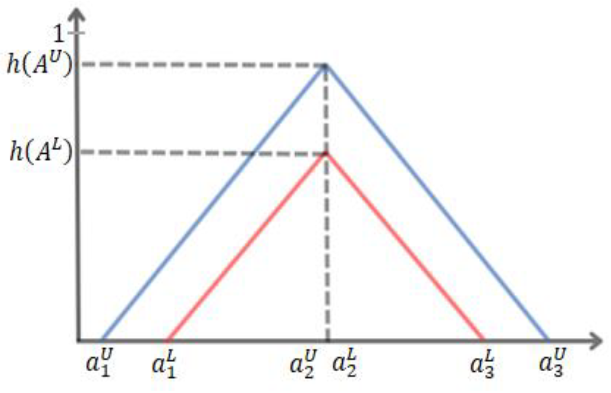
Figure 3.
The QFD process for green supplier selection problem.
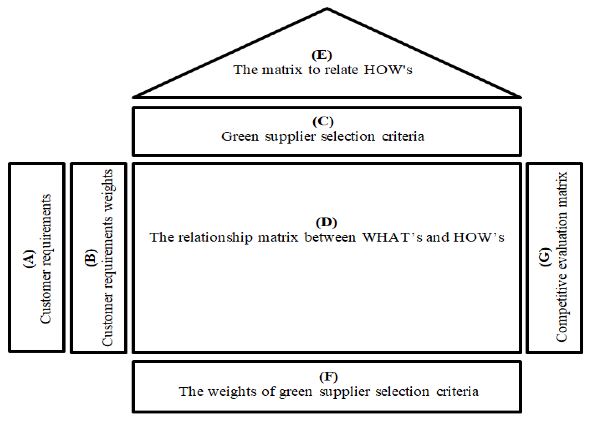
Figure 4.
The DEMATEL causal diagram for CRs.
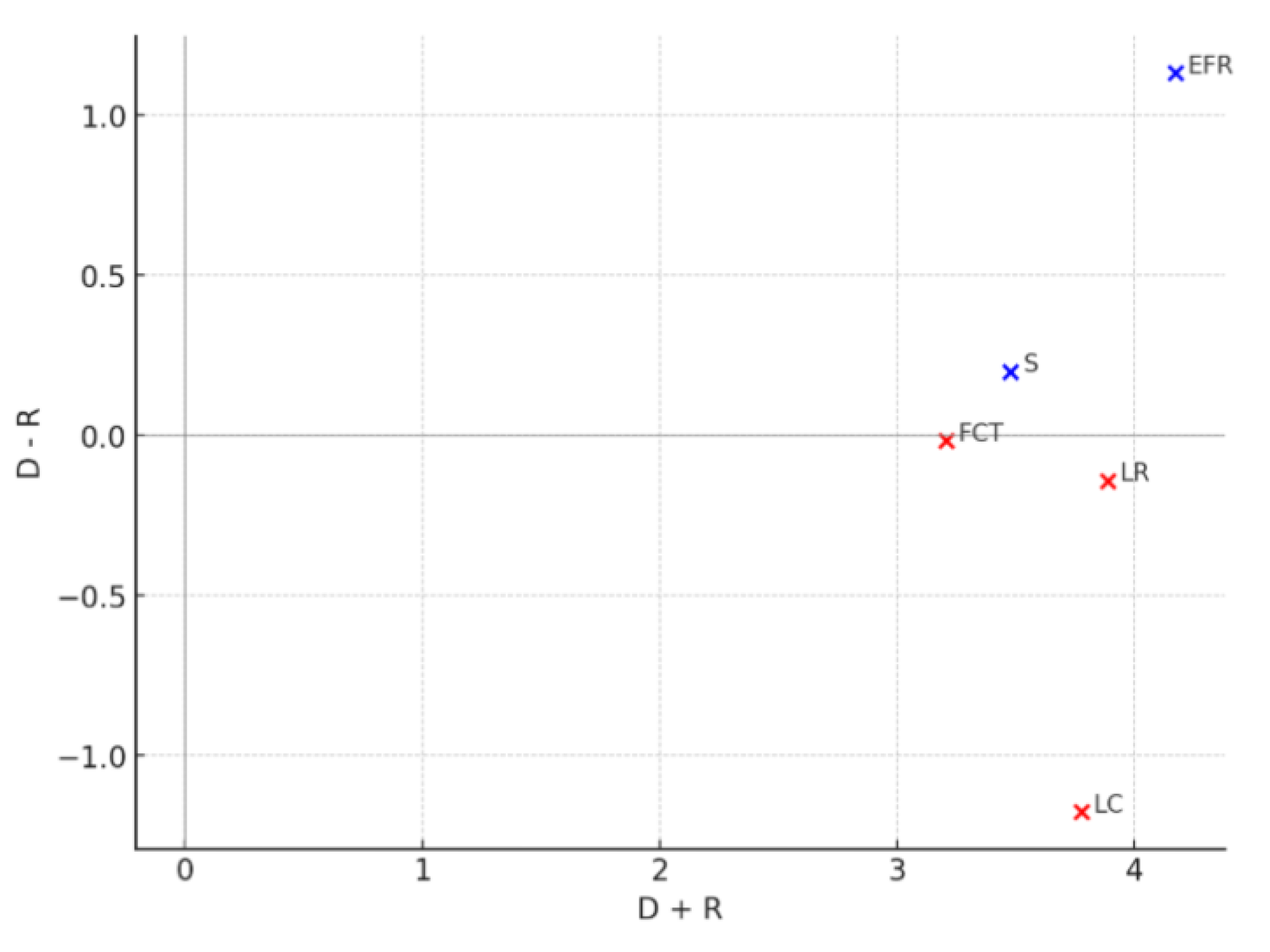
Figure 5.
DEMATEL diagram for the green supplier selection problem.
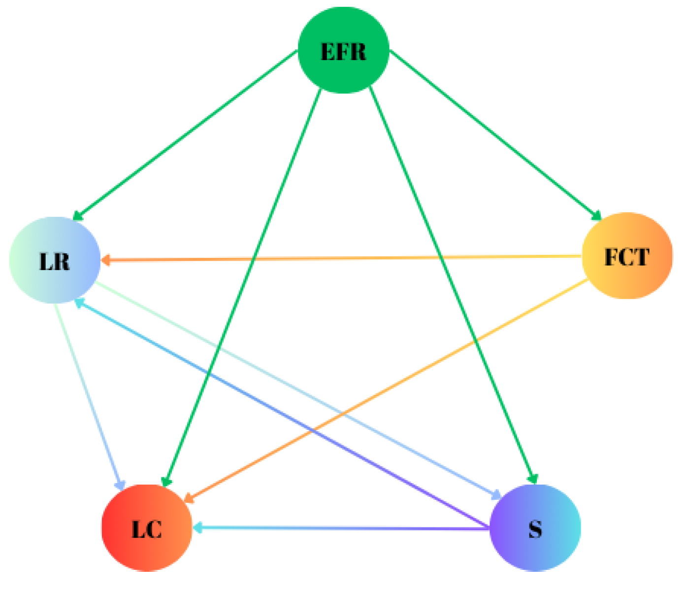
Figure 6.
Weights of Green Supplier Selection Criteria.

Figure 7.
Ranking performance of the alternatives based on the DEMATEL-QFD-IT2 Fuzzy VIKOR method.
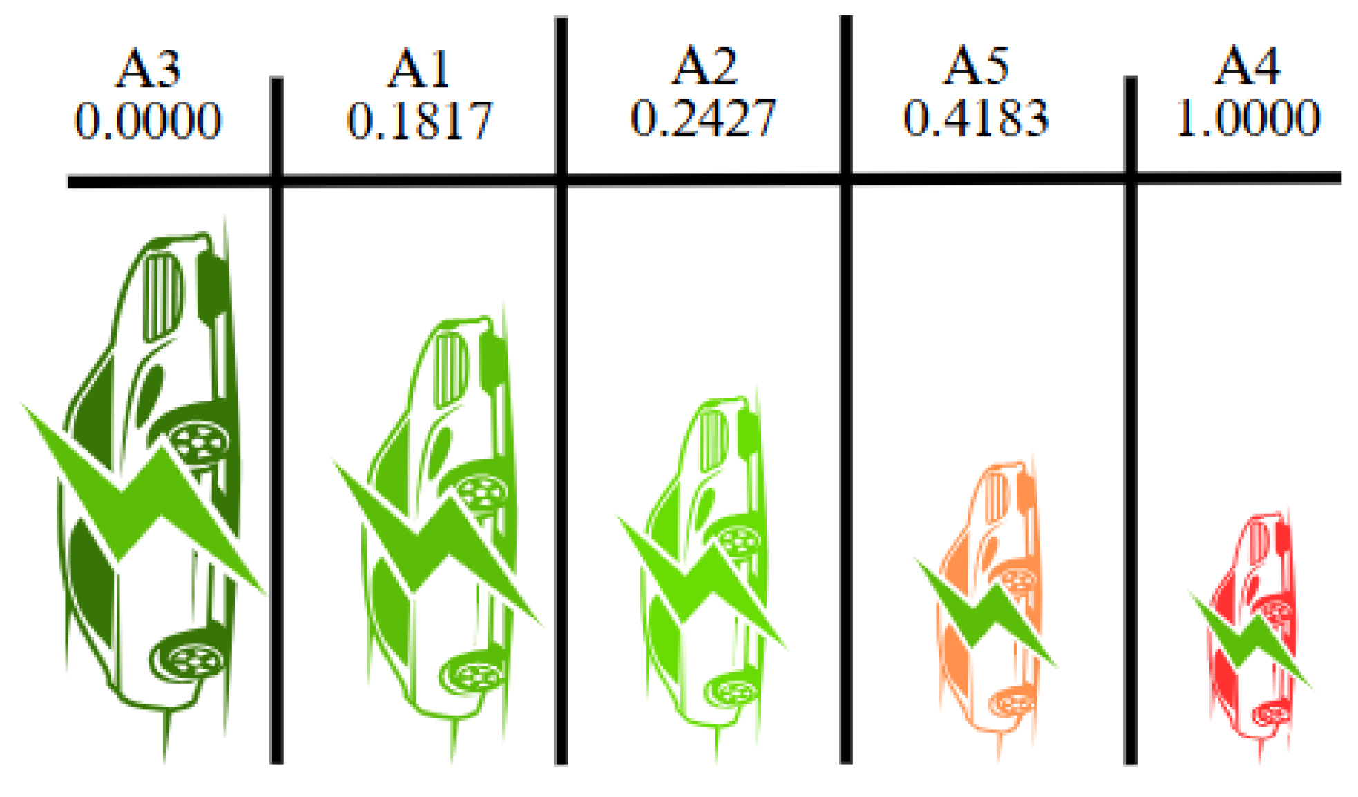

Table 1.
Summary of Previous Research on Electric Vehicles and Battery Selection.
| Author / Authors | Applied Method | Application Area |
| [8] | ORESTE method | Automotive-Battery Supplier Selection |
| [9] | Fuzzy QFD- Multiple regression Method | Automotive - Hybrid electric vehicles |
| [6] | Type-2 Fuzzy TOPSIS, Type-2 Fuzzy Hamming | Energy-Battery industry |
| [10] | Classical VIKOR- Fuzzy VIKOR | Transportation-Energy-Sensors |
| [11] | Fuzzy DEMATEL- LPWBN | Automotive - Electric vehicle - Battery supplier selection |
| [12] | DEMATEL-ISM | Automotive - Electric vehicle selection |
Table 2.
Customer Requirements and Green Supplier Criteria.
| Customer Requirements (Customer Demands) (CRs) | Explanation |
| Long range (LR) | It is the maximum distance that an electric vehicle can travel on a single full charge. |
| Fast charging time (FCT) | It refers to the time required for the battery to reach a specific charge level. |
| Safety (S) | It refers to the level of protection the vehicle and battery provide to the user against physical hazards. |
| Environmental friendliness and recyclability (EFR) | It refers to the minimal environmental impact of the battery's production, use, and disposal processes, as well as the inclusion of recyclable materials. |
| Low cost (LC) | It refers to the minimal impact of the battery on the vehicle's price or ensuring that its total cost remains at an acceptable level. |
| Green Supplier Selection Criteria | Explanation |
| Carbon Footprint (CO₂ Emissions) (CF) | It refers to the total greenhouse gas emissions (especially CO₂) generated throughout the process from raw material extraction to production, transportation, and usage of the battery. Low emissions are crucial for reducing environmental impacts. |
| Waste Management and Recycling Rate (WMRR) | It refers to how much of the battery can be recycled when its lifespan ends and how environmentally friendly this process is. A high recycling rate reduces resource waste and environmental pollution. |
| Use of Toxic and Critical Materials (TCMU) | It refers to the amount and type of materials used in the battery that are harmful to the environment and human health (e.g., cobalt, lead, fluoride electrolytes) or are at risk in terms of sourcing. Reducing the use of such materials is important both environmentally and ethically. |
| Use of Green Energy (GEU) | It refers to whether renewable energy sources (such as solar, wind, etc.) are used in the battery production processes. The use of green energy significantly reduces the environmental impact of the production process. |
| Energy Efficiency and Lifetime Impact (EELI) | It refers to how efficiently the battery provides energy and the total environmental impact throughout its entire life cycle. Long-lasting and highly efficient batteries reduce resource usage and waste generation |
Table 3.
The evaluated alternatives and the characteristics of the alternatives according to the green supplier criteria.
Table 3.
The evaluated alternatives and the characteristics of the alternatives according to the green supplier criteria.
| Abbreviation of the Alternatives | Battery Type / Criteria | Carbon Footprint (CO2 Emissions) | Recycling and Waste Management | Use of Toxic / Critical Materials | Use of Green Energy | Energy Efficiency and Lifetime Impact |
| A1 | NMC (Li-ion) |
High Intensive mining and processing process |
Medium It has existing infrastructure but is costly |
High Contains Cobalt and Nickel |
Low-Medium Typically produced using fossil energy |
Medium-High Good range but limited cycle life |
| A2 | LFP (LiFePO₄) |
Medium Simpler structure, production with lower energy |
High Easy and safe recycling |
Low Does not contain critical materials |
Medium-High Production is increasing with solar energy |
High Long cycle life and stable performance |
| A3 | Solid-State |
Medium-High Its production is complex; however, there is potential for cost reduction |
Medium As an emerging system, it encompasses both advantages and disadvantages |
Low-Medium It may vary depending on the material selection |
High (Objective) It is planned to increase the use of clean energy in production in the future. |
Very High Very long lifespan and high energy density |
| A4 | Li-S (Lithium Sulfur) |
Medium Lightweight material but inefficient production |
Low Sulfur-based structure poses challenges in recycling |
Low Does not contain critical materials |
Low In R&D-focused production, conventional energy is typically used |
Medium High capacity but short lifespan |
| A5 | Sodium-Ion |
Low Abundant resources, low-temperature production |
High Easy recycling due to its simple structure |
Low Does not contain toxic materials |
High Low temperature and production are easy with green energy |
Medium Low energy density, but durable structures are possible |
Table 4.
The initial basic relationship matrix (A).
| CRs | LR | FCT | S | EFR | LC |
| LR | 0 | 1 | 2 | 2 | 3 |
| FCT | 2 | 0 | 1 | 1 | 3 |
| S | 3 | 2 | 0 | 1 | 2 |
| EFR | 3 | 3 | 3 | 0 | 3 |
| LC | 1 | 1 | 1 | 2 | 0 |
Table 5.
The normalized direct relationship matrix (X) for CRs.
| CRs | LR | FCT | S | EFR | LC |
| LR | 0.0000 | 0.0833 | 0.1667 | 0.1667 | 0.2500 |
| FCT | 0.1667 | 0.0000 | 0.0833 | 0.0833 | 0.2500 |
| S | 0.2500 | 0.1667 | 0.0000 | 0.0833 | 0.1667 |
| EFR | 0.2500 | 0.2500 | 0.2500 | 0.0000 | 0.2500 |
| LC | 0.0833 | 0.0833 | 0.0833 | 0.1667 | 0.0000 |
Table 6.
The total impact matrix (T) for CRs. (tij* > 0.3704).
| CRs | LR | FCT | S | EFR | LC |
| LR | 0.2810 | 0.3055 | 0.3752* | 0.3619 | 0.5497* |
| FCT | 0.3732* | 0.1844 | 0.2693 | 0.2668 | 0.5010* |
| S | 0.4791* | 0.3575 | 0.2233 | 0.2926 | 0.4862* |
| EFR | 0.6029* | 0.5221* | 0.5279* | 0.3038 | 0.6952* |
| LC | 0.2782 | 0.2409 | 0.2436 | 0.2941 | 0.2439 |
Table 7.
The calculation of D and R vectors.
| CRs | Dk (Influencing) | Rk (Influenced) |
| LR | 1.8733 | 2.0144 |
| FCT | 1.5947 | 1.6104 |
| S | 1.8387 | 1.6393 |
| EFR | 2.6519 | 1.5192 |
| LC | 1.3007 | 2.4760 |
Table 8.
The total and net impact values for each CRs.
| CRs | D + R | D - R | Group |
| LR | 3.8877 | -0.1411 | Conclusion |
| FCT | 3.2051 | -0.0157 | Conclusion |
| S | 3.4780 | 0.1994 | Reason |
| EFR | 4.1711 | 1.1327 | Reason |
| LC | 3.7767 | -1.1753 | Conclusion |
Table 9.
Weights of the CRs.
| CRs | LR | FCT | S | EFR | LC |
| Ağırlıklar | 0.2099 | 0.1731 | 0.1878 | 0.2252 | 0.2039 |
Table 10.
QFD model for green supplier selection problem.
| HOW’s (CRs) | WHAT’s (Green Supplier Selection Criteria) | Weights of CRs | |||||
| CF | WMRR | TCMU | GEU | EELI | |||
| LR | 3 | 1 | 1 | 1 | 9 | 0.2099 | |
| FCT | 1 | 1 | 1 | 1 | 6 | 0.1731 | |
| S | 3 | 3 | 9 | 1 | 6 | 0.1878 | |
| EFR | 9 | 9 | 3 | 6 | 6 | 0.2252 | |
| LC | 3 | 3 | 6 | 3 | 3 | 0.2039 | |
| Absolute Importance Values | 4.0047 | 3.2093 | 3.9722 | 2.5337 | 6.0174 | ||
| Normalized Criterion Weights | 0.2029 | 0.1626 | 0.2013 | 0.1284 | 0.3049 | ||
Table 11.
The triangular fuzzy numbers that determine the importance levels of the criteria.
| Alternatives | Criteria | ||||
|
CF (Minimize) (0-10) |
WMRR (Maximize) (0-10) |
TCMU (Minimize) (0-10) |
GEU (Maximize) (0-10) |
EELI (Maximize) (0-10) |
|
| A1 | (2, 3.5, 5;1,1) (2.5, 3.5, 4.5;0.8, 0.8) |
(4, 5.5, 7;1,1) (4.4, 5.5, 6.6;0.8, 0.8) |
(1, 2.5, 4;1,1) (1.3, 2.5, 3.7;0.8, 0.8) |
(4, 5, 6;1,1) (4.2, 5, 5.8;0.8, 0.8) |
(5, 6, 7;1,1) (5.2, 6, 6.8;0.8, 0.8) |
| A2 | (5, 6.5, 8;1,1) (5.4, 6.5, 7.6;0.8, 0.8) |
(7, 8.5, 10;1,1) (7.3, 9, 9.7;0.8, 0.8) |
(8, 9, 10;1,1) (8.4, 9, 9.6;0.8, 0.8) |
(5, 7, 8;1,1) (5.6, 7, 7.4;0.8, 0.8) |
(7, 9, 10;1,1) (7.3, 9, 9.7;0.8, 0.8) |
| A3 | (5, 6, 7;1,1) (5.5, 6, 6.5;0.8, 0.8) |
(4.5, 5.5, 6.5;1,1) (5, 5.5, 6;0.8, 0.8) |
(4.5, 6, 7.5;1,1) (5, 6, 7;0.8, 0.8) |
(7, 9, 10;1,1) (7.6, 9, 9.4;0.8, 0.8) |
(8, 9, 10;1,1) (8.3, 9, 9.7;0.8, 0.8) |
| A4 | (5.5, 6.4, 8;1,1) (6, 6.4, 7.5;0.8, 0.8) |
(3, 4, 5.5;1,1) (3.3, 4, 5.2;0.8, 0.8) |
(6, 7.5, 9;1,1) (6.6, 7.5, 8.4;0.8, 0.8) |
(3, 4, 5;1,1) (3.4, 4, 4.6;0.8, 0.8) |
(2, 3.5, 5;1,1) (2.5, 4, 4.5;0.8, 0.8) |
| A5 | (8, 9, 10;1,1) (8.5, 9, 9.5;0.8, 0.8) |
(9, 9.5, 10;1,1) (9.2, 9.5, 9.8;0.8, 0.8) |
(9, 9.5, 10;1,1) (9.3, 9.5, 9.7;0.8, 0.8) |
(9, 9.5, 10;1,1) (9.2, 9.5, 9.8;0.8, 0.8) |
(5, 6, 7;1,1) (5.5, 6, 6.5;0.8, 0.8) |
Table 12.
Best and worst values calculated for each criterion.
| Criterion | Best | |
| CF (Minimize) | (2, 3.5, 5;1,1) (2.5, 3.5, 4.5;0.8, 0.8) |
(8, 9, 10;1,1) (8.5, 9, 9.5;0.8, 0.8) |
| WMRR (Maximize) | (9, 9.5, 10;1,1) (9.2, 9.5, 9.8;0.8, 0.8) |
(3, 4, 5.5;1,1) (3.3, 4, 5.2;0.8, 0.8) |
| TCMU (Minimize) | (1, 2.5, 4;1,1) (1.3, 2.5, 3.7;0.8, 0.8) |
(9, 9.5, 10;1,1) (9.3, 9.5, 9.7;0.8, 0.8) |
| GEU (Maximize) | (9, 9.5, 10;1,1) (9.2, 9.5, 9.8;0.8, 0.8) |
(3, 4, 5;1,1) (3.4, 4, 4.6;0.8, 0.8) |
| EELI (Maximize) | (8, 9, 10;1,1) (8.3, 9, 9.7;0.8, 0.8) |
(2, 3.5, 5;1,1) (2.5, 4, 4.5;0.8, 0.8 |
Table 13.
Interval type-2 fuzzy membership values calculated for the prior and values of each alternative.
Table 13.
Interval type-2 fuzzy membership values calculated for the prior and values of each alternative.
| Alternatives |
CF (Minimize) |
WMRR (Maximize) |
TCMU (Minimize) |
GEU (Maximize) |
EELI (Maximize) |
| A1 | (0, 0, 0;1,1) (0, 0, 0;0.8, 0.8) |
(0.1355, 0.1183, 0.1084;1,1) (0.1323, 0.1183, 0.1131;0.8, 0.8) |
(0, 0, 0;1,1) (0, 0, 0;0.8, 0.8) |
(0.1070, 0.1051, 0.1027;1,1) (0.1107, 0.1051, 0.0988;0.8, 0.8) |
(0.1525, 0.1663, 0.1829;1,1) (0.1630, 0.1829, 0.1700;0.8, 0.8) |
| A2 | (0.1015, 0.1107, 0.1217;1,1) (0.0981, 0.1107, 0.1258;0.8, 0.8) |
(0.0542, 0.0296, 0.0000;1,1) (0.0524, 0.0148, 0.0035;0.8, 0.8) |
(0.1761, 0.1869, 0.2013;1,1) (0.1787, 0.1869, 0.1979;0.8, 0.8) |
(0.0856, 0.0584, 0.0514;1,1) (0.0797, 0.0584, 0.0593;0.8, 0.8) |
(0.0508, 0.0000, 0.0000;1,1) (0.0526, 0.0000, 0.0000;0.8, 0.8) |
| A3 | (0.1015, 0.0922, 0.0812;1,1) (0.1015, 0.0922, 0.0812; 0.8, 0.8) |
(0.1220, 0.1183, 0.1138;1,1) (0.1157, 0.1183, 0.1343;0.8, 0.8) |
(0.0881, 0.1007, 0.1174;1,1) (0.0931, 0.1007, 0.1107;0.8, 0.8) |
(0.0428, 0.0117, 0.0000;1,1) (0.0354, 0.0117, 0.0099;0.8, 0.8) |
(0, 0, 0;1,1) (0, 0, 0;0.8, 0.8) |
| A4 | (0.2367, 0.2213, 0.2029;1,1) (0.2266, 0.2213, 0.2151; 0.8, 0.8) |
(0.1626, 0.1626, 0.1463;1,1) (0.1626, 0.1626, 0.1626;0.8, 0.8) |
(0.1258, 0.1438, 0.1678;1,1) (0.1334, 0.1438, 0.1577;0.8, 0.8) |
(0.1284, 0.1284, 0.1284;1,1) (0.1284, 0.1284, 0.1284;0.8, 0.8) |
(0.3049, 0.3049, 0.3049;1,1) (0.3049, 0.3049, 0.3049;0.8, 0.8) |
| A5 | (0.2029, 0. 2029, 0. 2029;1,1) (0.1961, 0.2029, 0.2110; 0.8, 0.8) |
(0, 0, 0;1,1) (0, 0, 0;0.8, 0.8) |
(0.2013, 0.2013, 0.2013;1,1) (0.2013, 0.2013, 0.2013;0.8, 0.8) |
(0, 0, 0;1,1) (0, 0, 0;0.8, 0.8) |
(0.1525, 0.1663, 0.1839;1,1) (0.1472, 0.1829, 0.1876;0.8, 0.8) |
Table 14.
Interval type-2 fuzzy and values calculated for each alternative.
| Alternatives | (The sum of all criteria) | (he largest criterion value) |
| A1 | (0.3950, 0.3897, 0.3940;1,1) (0.4060, 0.4063, 0.3819;0.8, 0.8) |
(0.1525, 0.1663, 0.1829;1,1) (0.1630, 0.1829, 0.1700;0.8, 0.8) |
| A2 | (0.4682, 0.3856, 0.3744;1,1) (0.4615, 0.3708, 0.3865;0.8, 0.8) |
(0.1761, 0.1869, 0.2013;1,1) (0.1787, 0.1869, 0.1979;0.8, 0.8) |
| A3 | (0.3544, 0.3229, 0.3124;1,1) (0.3457, 0.3229, 0.3361;0.8, 0.8) |
(0.1220, 0.1183, 0.1174;1,1) (0.1157, 0.1183, 0.1343;0.8, 0.8) |
| A4 | (0.9584, 0.9610, 0.9503;1,1) (0.9559, 0.9610, 0.9684;0.8, 0.8) |
(0.3049, 0.3049, 0.3049;1,1) (0.3049, 0.3049, 0.3049;0.8, 0.8) |
| A5 | (0.5567, 0.5705, 0.5881;1,1) (0.5446, 0.5871, 0.5999;0.8, 0.8) |
(0.2029, 0.2029, 0.2029;1,1) (0.2013, 0.2029, 0.2110;0.8, 0.8) |
Table 15.
Fuzzy VIKOR index () values calculated for the alternative.
| Alternative | VIKOR Index () |
| A1 | (0.1170, 0.1810, 0.2386;1, 1) (0.1744, 0.2384, 0.1408;0.8, 0.8) |
| A2 | (0.2421, 0.2329, 0.2723;1, 1) (0.2614, 0.2213, 0.2263;0.8, 0.8) |
| A3 | (0.0000, 0.0000, 0.00000;1, 1) (0.0000, 0.0000, 0.0000;0.8, 0.8) |
| A4 | (1.0000, 1.0000, 1.00000;1, 1) (1.0000, 1.0000, 1.0000;0.8, 0.8) |
| A5 | (0.3886, 0.4207, 0.4441;1, 1) (0.3892, 0.4337, 0.4334;0.8, 0.8) |
| has been taken | |
Table 16.
Defuzzified (crips) values calculated for each alternative.
| Alternative | |
| A1 | 0.1817 |
| A2 | 0.2427 |
| A3 | 0.0000 |
| A4 | 1.0000 |
| A5 | 0.4183 |
Table 17.
Selection and ranking performance of the alternatives.
| Alternatives | A3 | A1 | A2 | A5 | A4 |
| Values of Alternatives Calculated Using the DEMATEL-QFD-IT2 F-VIKOR Method | 0.0000 | 0.1817 | 0.2427 | 0.4183 | 1.0000 |
| Ranking Performance of Alternatives | 1 | 2 | 3 | 4 | 5 |
Disclaimer/Publisher’s Note: The statements, opinions and data contained in all publications are solely those of the individual author(s) and contributor(s) and not of MDPI and/or the editor(s). MDPI and/or the editor(s) disclaim responsibility for any injury to people or property resulting from any ideas, methods, instructions or products referred to in the content. |
© 2025 by the authors. Licensee MDPI, Basel, Switzerland. This article is an open access article distributed under the terms and conditions of the Creative Commons Attribution (CC BY) license (http://creativecommons.org/licenses/by/4.0/).
Copyright: This open access article is published under a Creative Commons CC BY 4.0 license, which permit the free download, distribution, and reuse, provided that the author and preprint are cited in any reuse.


