
Submitted:
23 April 2025
Posted:
24 April 2025
You are already at the latest version
Abstract
The practical utility of Noisy Intermediate-Scale Quantum (NISQ) processors depends critically on their performance under demanding computational loads. We investigated the impact of circuit depth on the 127-qubit superconducting processor ibm_brisbane by executing stress-test circuits utilizing all available qubits. These circuits consisted of repeated layers combining random single-qubit rotations and linear chains of Controlled-Z entangling gates. We systematically increased the ideal circuit depth from 1 up to 30 layers, resulting in transpiled circuits ranging from approximately 550 to over 15,000 gates (optimization level 2). Using the qiskit-ibm-runtime Sampler primitive with 4096 shots and default error mitigation, we successfully obtained results for ideal depths up to 22 (transpiled depth ~11.7k gates), beyond which platform usage limits prevented execution. Our central finding is the immediate onset of noise saturation: the output distribution reached maximum sample entropy (12.0 bits) and exhibited near-zero average single-qubit Z magnetization even at the shallowest depth tested (ideal depth 1, transpiled depth ~550). These noise-dominated characteristics persisted despite significant increases in transpiled circuit depth. This demonstrates that for these specific full-width, complex random circuits, noise overwhelms the computation almost instantaneously on this device under default settings, highlighting the profound challenge of achieving computational fidelity for deep, wide algorithms in the NISQ era without advanced error handling.

Keywords:
quantum computing
; NISQ
; IBM brisbane
; 127 qubits
; stress testing
; quantum circuits
; circuit depth
; noise saturation
; random circuits
; entangling gates
; CZ gates
; transpilation
; qiskit
; qiskit-ibm-runtime
; error mitigation
; quantum volume
; shannon entropy
; Z magnetization
; superconducting qubits
; computational fidelity
; decoherence
Introduction
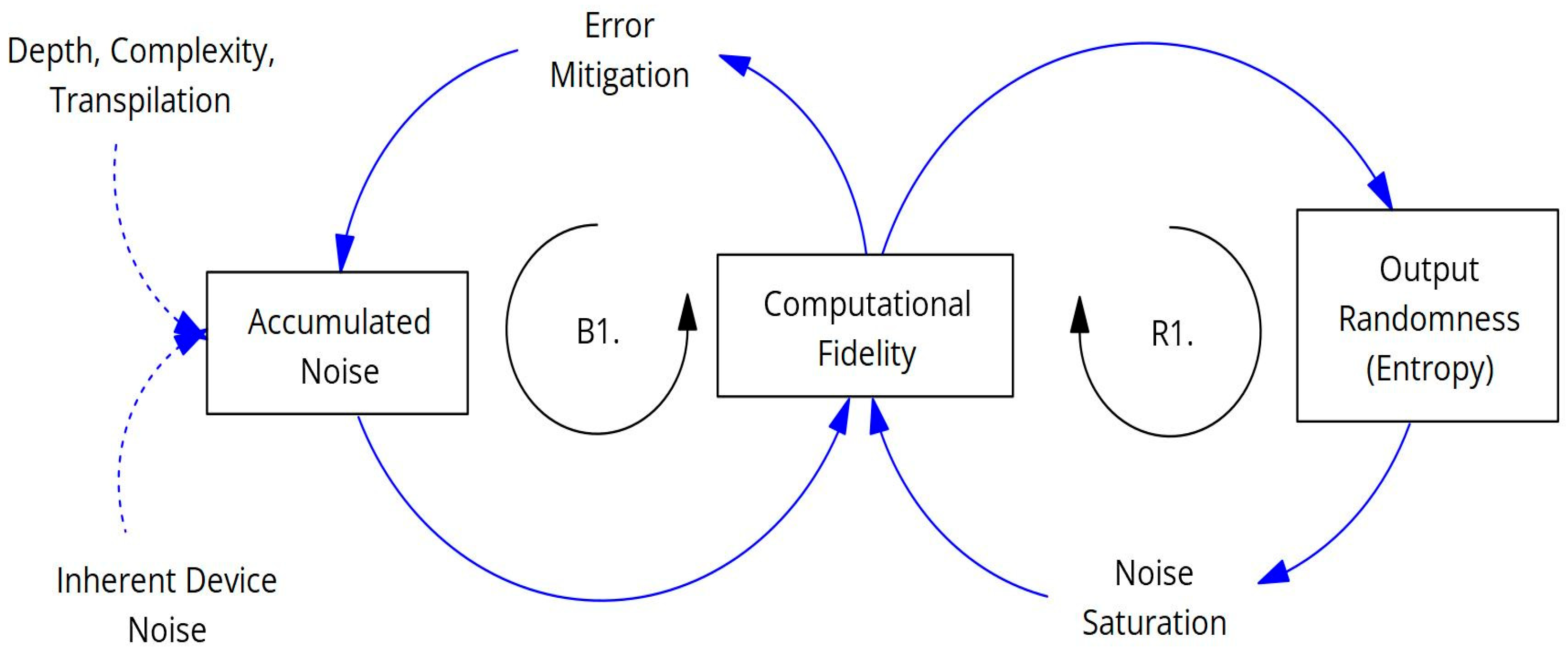
The causal loop diagram illustrates the dynamics of noise and its impact on quantum computation performance. Factors such as increasing circuit depth, complexity, and the transpilation process, alongside inherent device noise, contribute to Accumulated Noise within the quantum system. This accumulated noise fundamentally degrades Computational Fidelity, representing the accuracy of the computation, forming a balancing loop (B1) where higher noise leads to lower fidelity. While Error Mitigation strategies aim to counteract this degradation and improve fidelity, the relationship between fidelity and the final Output Randomness (measured by entropy) forms another loop (R1). Decreasing computational fidelity results in increased output randomness, as the quantum state loses coherence and approaches a uniform noise distribution. Ultimately, Noise Saturation, a state where noise completely dominates, directly drives output randomness to its maximum, signifying a collapse of computational fidelity and rendering the output indistinguishable from random noise, a phenomenon observed even at shallow depths in the experiments detailed herein.
Figure 1.
Causal Loop Diagram Illustrating Noise Impact on Computational Fidelity and Output Randomness.
Figure 1.
Causal Loop Diagram Illustrating Noise Impact on Computational Fidelity and Output Randomness.
The current development of quantum computation is situated in the Noisy Intermediate-Scale Quantum (NISQ) era, characterized by processors containing tens to hundreds of qubits that, while offering potential for exploring complex quantum phenomena, are simultaneously limited by significant operational noise and finite qubit coherence times (Preskill, 2018). Evaluating the practical capabilities of these NISQ processors requires characterization methods that go beyond component-level metrics, such as isolated gate fidelities (often measured by techniques like Randomized Benchmarking; Magesan et al., 2011) or holistic measures like Quantum Volume (Cross et al., 2019), which may not fully capture performance under high computational load involving full qubit utilization and deep circuits (Baldwin et al., 2022). It is particularly crucial to understand hardware performance under these demanding conditions, as noise accumulation—arising from constituent gate errors, environmental decoherence (e.g., due to TLS, radiation), and readout inaccuracies (Nielsen & Chuang, 2010; Klimov et al., 2018; Cardani et al., 2021)—fundamentally limits the complexity and achievable fidelity of quantum algorithms (Bharti et al., 2022).
To probe these operational boundaries, stress testing using specific classes of synthetic benchmark circuits serves as a valuable methodology. Such tests often employ circuits designed to generate high entanglement across the processor and involve a large number of gate operations, similar in spirit to random circuit sampling experiments used to benchmark device capabilities (Arute et al., 2019). These tests stress the device under conditions relevant to complex quantum simulations or future fault-tolerant computations. In this work, we utilize circuits composed of repeated layers of random single-qubit gates and fixed entangling operations to exert such stress across the entire processor width.
We perform this stress test on ibm_brisbane, a 127-qubit superconducting quantum processor from IBM Quantum's 'Eagle' family (Chow et al., 2021), accessed via the IBM Quantum platform using qiskit-ibm-runtime. Our primary research objective is to characterize how the output fidelity of this large-scale device behaves as circuit depth is systematically increased while utilizing all available qubits. Specifically, we investigate the relationship between logical circuit depth (number of layers) and output distribution metrics, namely Shannon entropy and average single-qubit Z magnetization, to determine the approximate depth at which noise becomes the dominant factor, effectively randomizing the computation for this class of complex, entangling circuits.
Methods
All quantum experiments were executed on the ibm_brisbane quantum processor, a 127-qubit device based on superconducting transmon qubit technology (Gambetta et al., 2017; Chow et al., 2021), accessed via the IBM Quantum cloud platform. This processor utilizes a Heavy Hex qubit connectivity topology, characteristic of IBM's 'Eagle' processor family (Chow et al., 2021). Communication with the platform and job submission were handled using the qiskit-ibm-runtime Python package, version 0.37.0 (IBM Quantum, n.d.-c). Experiments were conducted around April 21-22, 2025. The primary software stack included Python 3, Qiskit (Qiskit Development Team, 2024), NumPy, Pandas for data handling, and Matplotlib for visualization.
Figure 2.
Example Quantum Circuit Structure for Stress Test (Illustrative N=4 qubits, Depth=2).
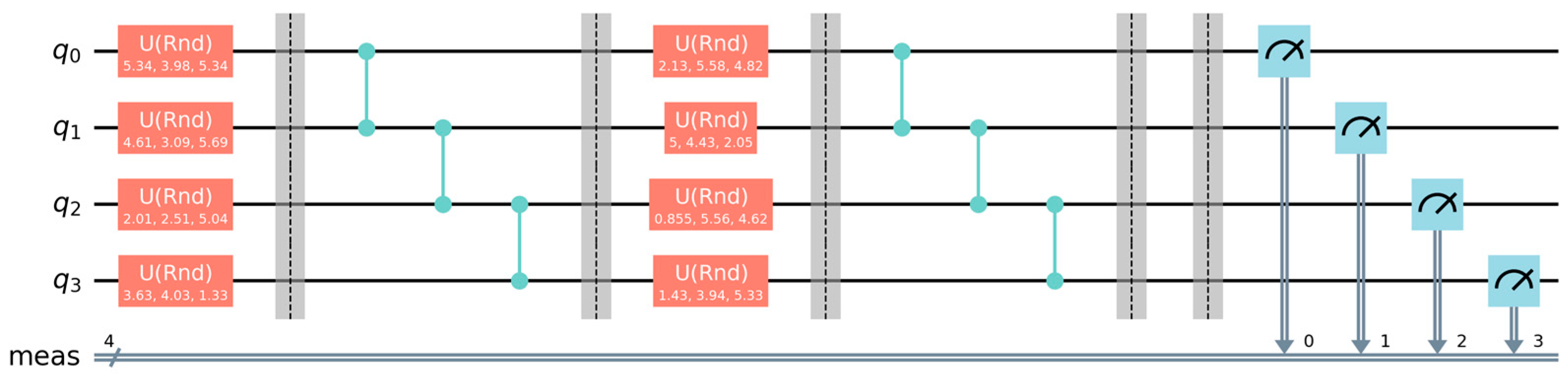
The quantum circuit structure above illustrates the layered structure of the benchmark circuits using a small example with N=4 qubits and an ideal depth d=2. To probe the system's performance under high computational load, we designed a synthetic benchmark circuit operating on all N=127 qubits, similar in spirit to random circuit sampling approaches used for benchmarking (Arute et al., 2019; Cross et al., 2019). The circuit structure consists of d repeated layers, where d is the "ideal depth" parameter varied in our experiments. Each layer is composed of two sub-layers: first, a layer of simultaneous random single-qubit universal rotations, implemented using Qiskit's U gate (U(θ,ϕ,λ)), where the angles θ,ϕ,λ for each qubit were drawn independently and uniformly from [0,2π); second, a layer of entangling gates, implemented as a linear chain of Controlled-Z (CZ) gates connecting qubit i to qubit i+1 for i ranging from 0 to N−2=125. Qiskit barrier instructions were inserted between sub-layers for logical clarity but have no physical effect during execution. Following the d layers, a final measurement in the computational (Z) basis was applied to all qubits using Qiskit's measure_all operation, mapping results to a single 127-bit classical register. We systematically varied the ideal depth parameter d across the range from 1 to 30.
Before execution, each constructed ideal circuit was transpiled specifically for the ibm_brisbane backend's instruction set architecture (ISA) and coupling map using the qiskit.compiler.transpile function (IBM Quantum, n.d.-b ). We used optimization_level=2 to balance optimization effort and compilation time; noise-aware or variability-aware compilation strategies were not explicitly employed (cf. Murali et al., 2019; Tannu & Qureshi, 2019). This process maps logical qubits to physical device qubits and decomposes logical gates into the hardware's native basis gate set (primarily ECR, SX, RZ, X, ID gates for IBM hardware). The resulting transpiled circuit depths ranged from approximately 550 gates (for d=1) to over 15,000 gates (for d=30), with corresponding total native gate counts ranging from ~1800 to over 60,000.
Jobs were submitted to the backend via the qiskit_ibm_runtime.Sampler primitive (V2 interface), managed within a qiskit_ibm_runtime.Session context for each job submission. A total of Nshots=4096 shots were requested for each circuit execution. Default runtime options were used by passing options= {} to the Sampler, implying default error mitigation settings were applied by the service (IBM Quantum, n.d.-a), likely including basic measurement error mitigation (e.g., Bravyi et al., 2021; van den Berg et al., 2023) but not more advanced techniques like Zero-Noise Extrapolation (Temme et al., 2017) for this set of experiments.
Completed job results were retrieved using the job.result() method. The raw measurement outcomes were obtained from the SamplerResult's data structure (result(0).data.meas.get_counts()), typically returned as a dictionary mapping hexadecimal string (representing measured states) to counts. Due to the observation of keys corresponding to integers larger than the expected 2127−1 range, each key k was processed by converting to an integer, applying a 127-bit mask (& ((1 << 127) - 1)), and reformatting to a fixed-length binary string to ensure correct interpretation of the 127-qubit outcomes. Counts from different raw keys mapping to the same 127-bit string were aggregated.
From the processed binary counts distribution p(x) for each run, we calculated several metrics:
- (i)
- The total number of unique observed 127-bit outcomes.
- (ii)
- The Shannon entropy H of the measured probability distribution p(x) over the output bitstrings x is calculated as:
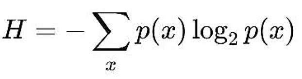
Where the sum is over all possible measurement outcomes (bitstrings) x, and p(x) is the observed probability of measuring bitstring x. The logarithm is base 2, so the entropy is measured in bits.
- (iii)
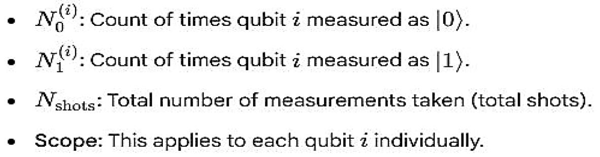
- The average magnetization (or expectation value of the Pauli-Z operator) for a specific qubit i, denoted ⟨Zi⟩, is calculated from the measurement counts as:
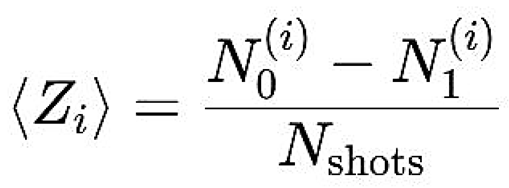
Where:
Results
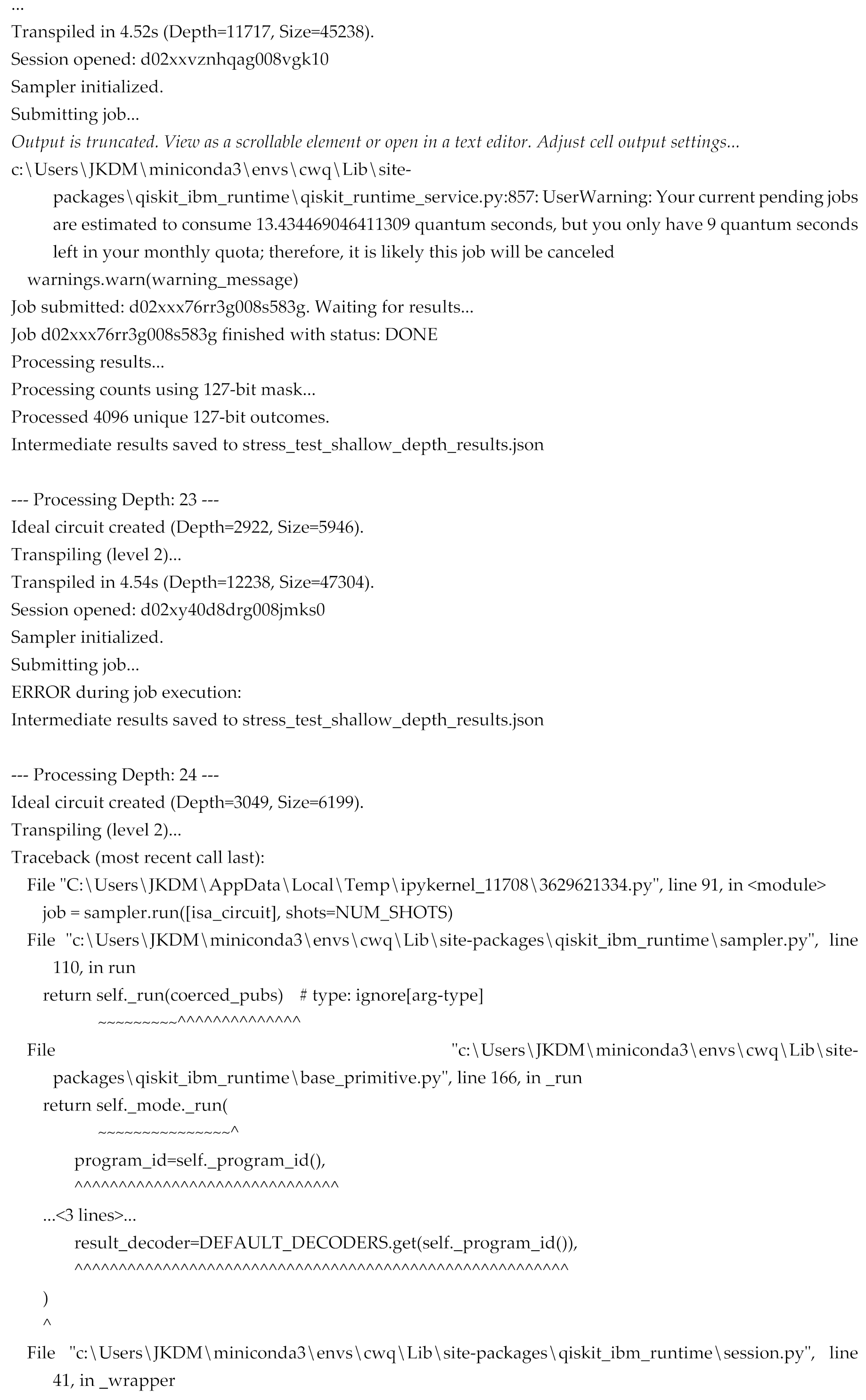
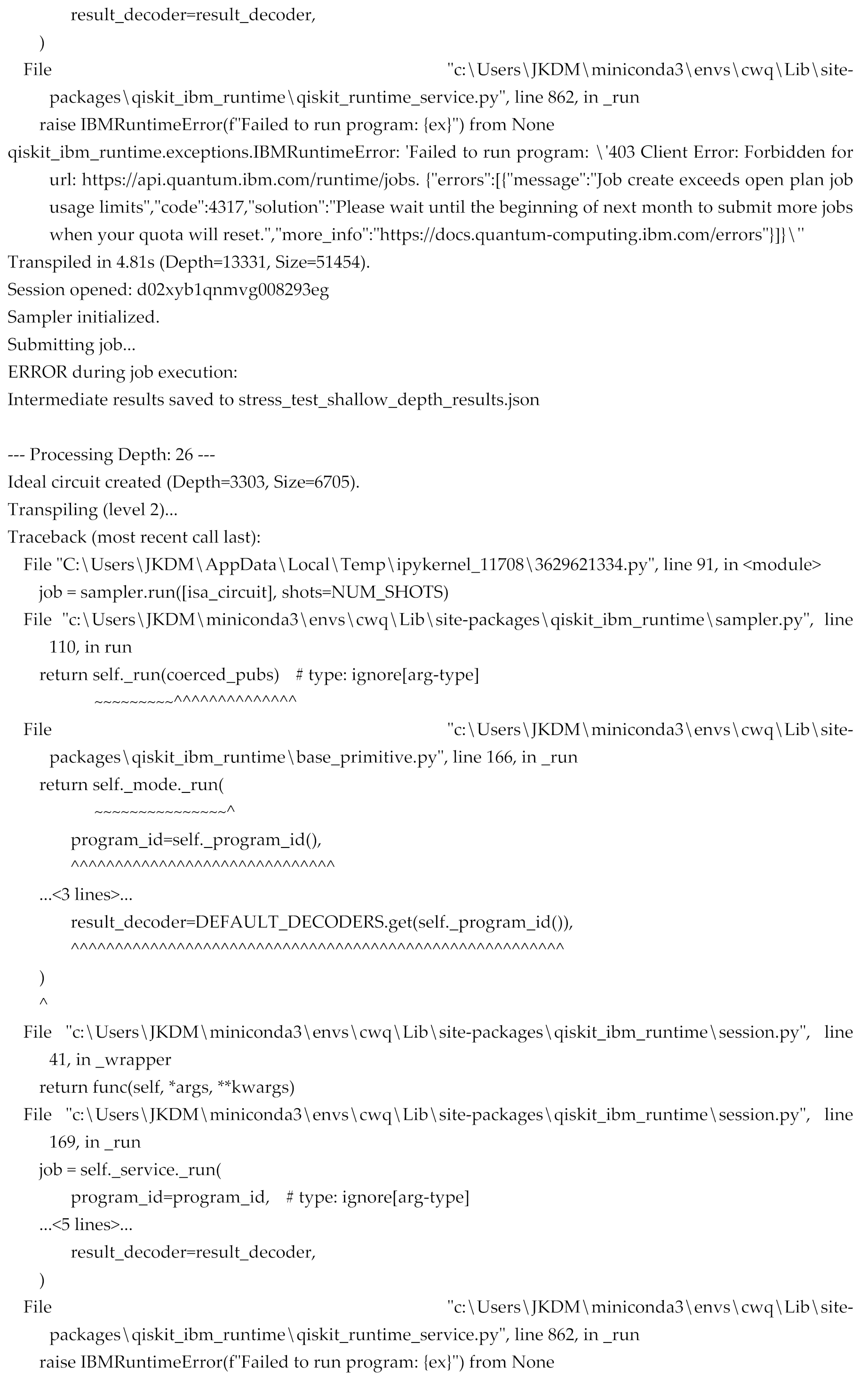
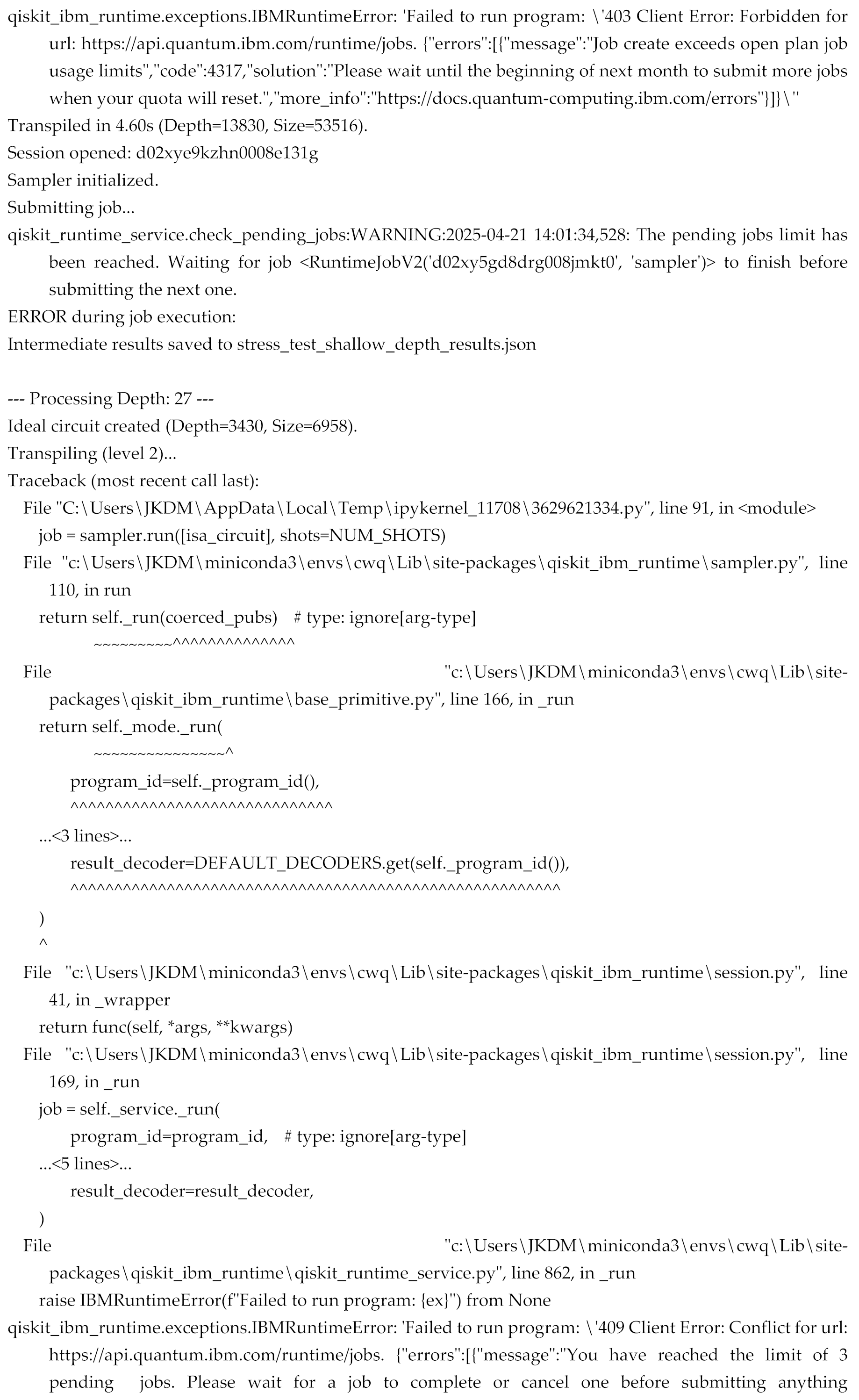
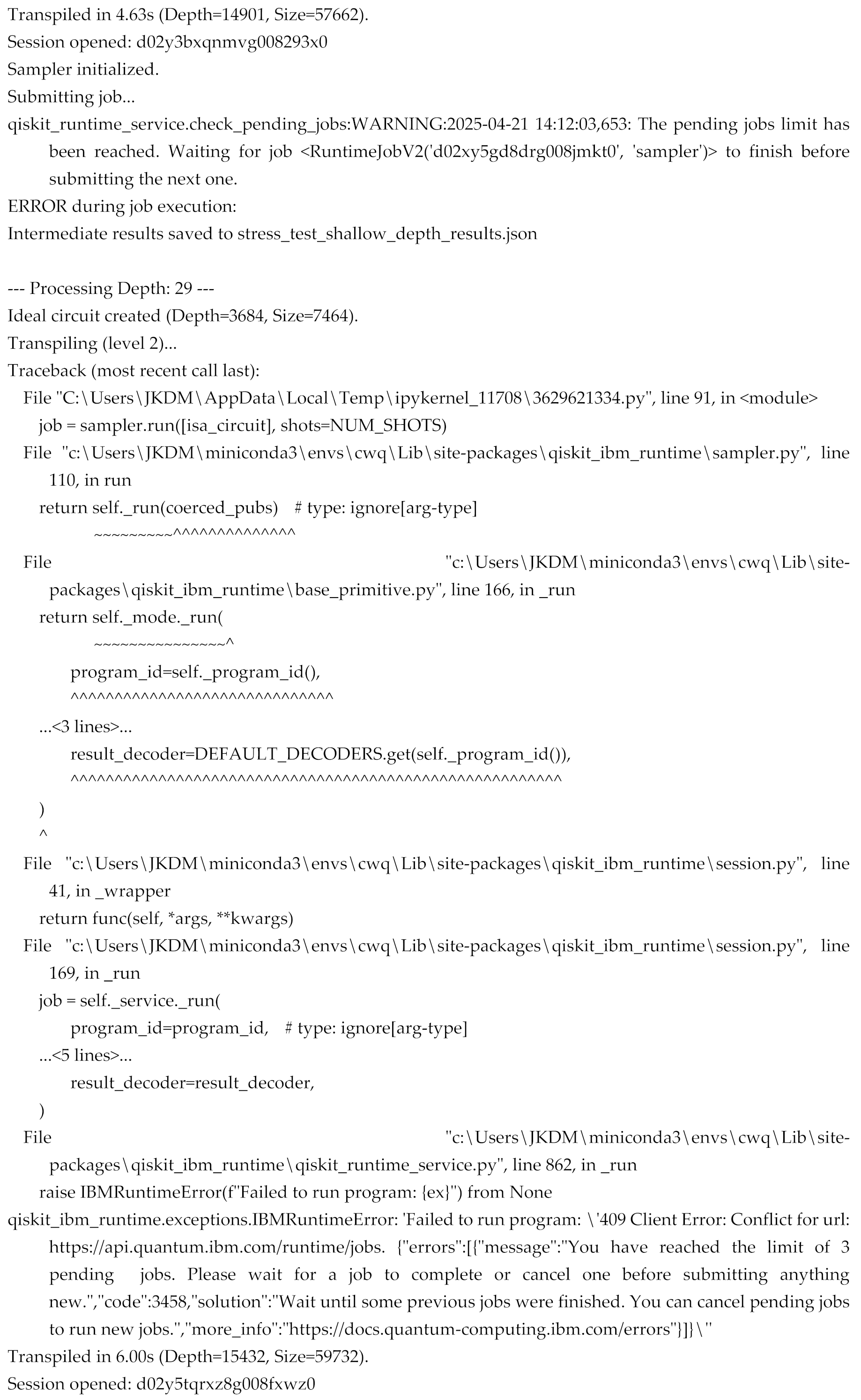
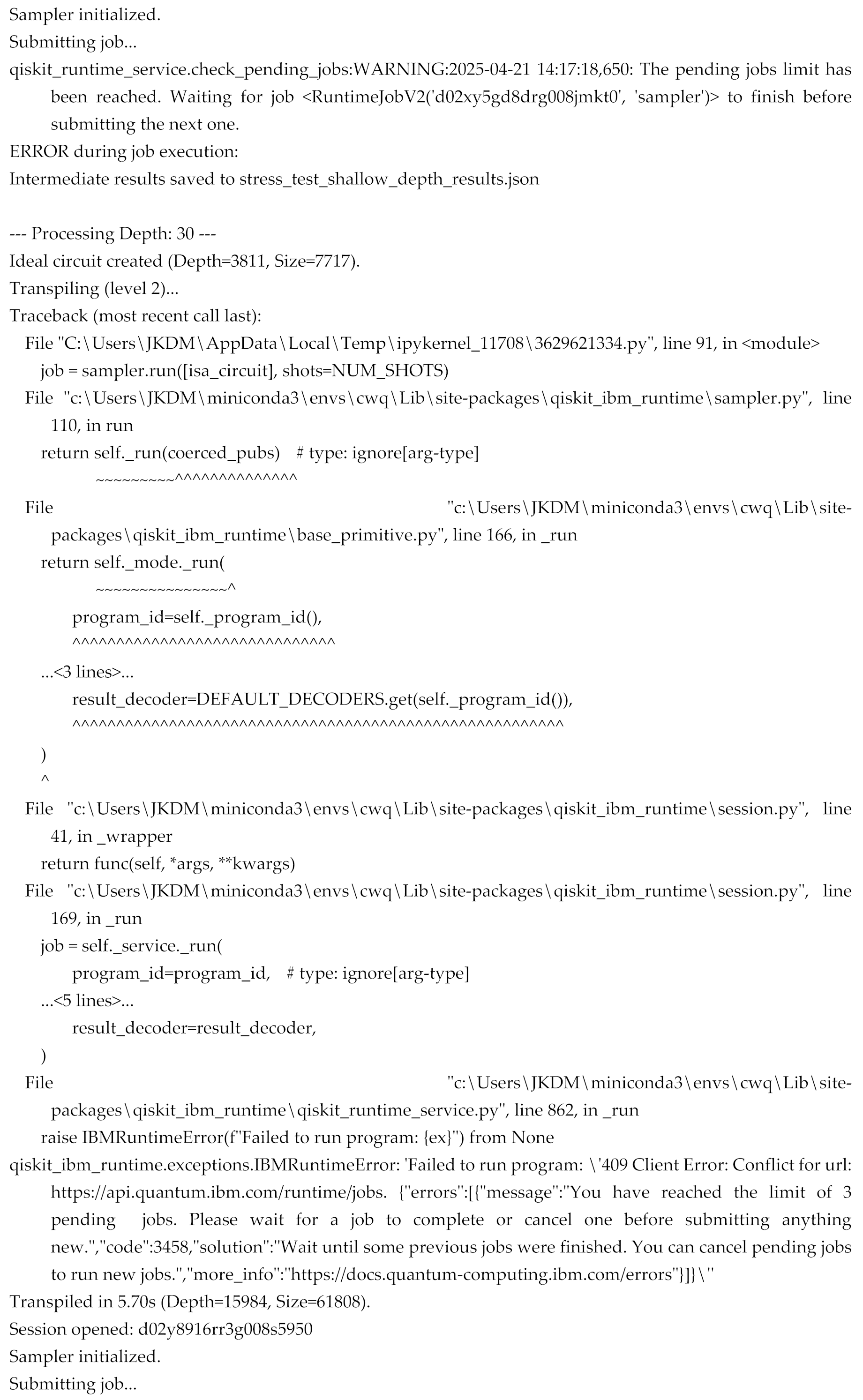
We executed the depth-scaling stress test circuits for ideal depths d ranging from 1 to 30 on the ibm_brisbane processor. A summary of the experimental runs and key resulting metrics is presented in Figure 4. Runs for ideal depths d=1 through d=22 completed successfully with status DONE. However, job submissions for d≥23 failed due to exceeding platform usage limits associated with the user account plan (specifically, initial failures indicated quota limits followed by subsequent failures due to exceeding the pending job limit). Consequently, detailed analysis is presented for the successful runs from d=1 to d=22.
The primary performance metrics as a function of ideal circuit depth are visualized in Figure 4. Panel (a) displays the Shannon entropy of the output distribution, calculated from the 4096 shots obtained for each completed run. The entropy immediately saturates at a value of 12.0 bits for d=1 (corresponding to a transpiled depth of ~550 gates) and remains constant at this value for all successfully executed depths up to d=22. This value corresponds to the maximum possible entropy for a distribution spread across 4096 unique outcomes (log2(4096)=12), indicating maximum randomness within the sample size achieved even at the shallowest depth. Panel (d) confirms this observation, showing that the number of unique measured bitstrings also saturated at the maximum possible value of 4096 for all depths from d=1 onwards.
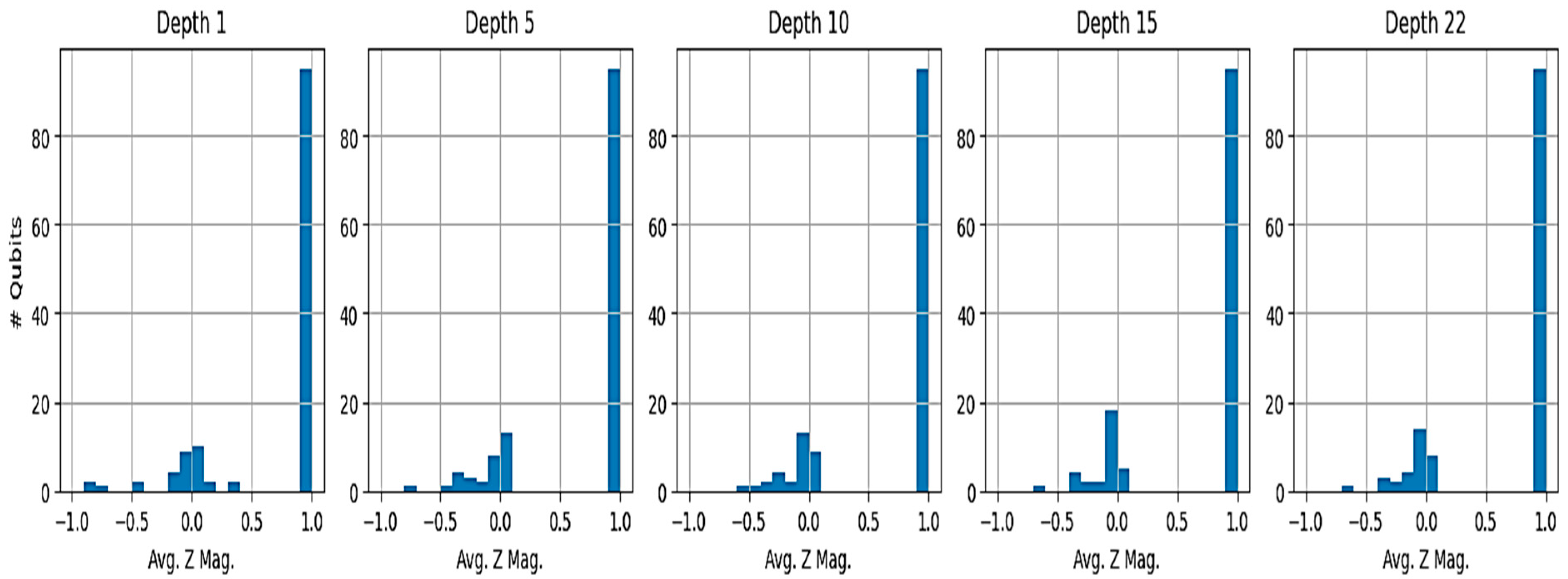
Further insight into the output state is provided by the single-qubit Z magnetization, ⟨Zi⟩. Figure 5 presents histograms of the ⟨Zi⟩ values calculated for all 127 qubits for several representative ideal circuit depths (d=1, 5, 10, 15, and 22). As shown in the figure, for all these depths, the distribution is tightly clustered around zero, indicating that, on average, each qubit yielded random outcomes (50% probability of measuring 0, 50% probability of measuring 1). This behavior was consistent across all successfully measured depths (d=1 through d=22), which is further supported by the low and stable standard deviation of the ⟨Zi⟩ values shown in Figure 4(b). This confirms the lack of any significant qubit bias towards ∣0⟩ or ∣1⟩, even as the computational workload increased significantly, evidenced by the near-linear growth in transpiled circuit depth shown in Figure 4(c). In summary, the key numerical findings demonstrate an immediate saturation of output randomness metrics (sample entropy, unique outcomes) and near-zero qubit magnetizations at the shallowest ideal depth tested (d=1), which persisted even as the transpiled circuit depth increased by over an order of magnitude across the successfully executed runs.
Discussion
The results presented in Section 3 compellingly indicate that for the specific class of wide (127-qubit), computationally intensive random circuits executed on ibm_brisbane, the system enters a regime dominated by noise almost instantaneously. The saturation of the Shannon entropy at the maximum possible value dictated by the sample size (12.0 bits for 4096 shots), combined with the observation of the maximum number (4096) of unique outcomes, occurs even at the shallowest ideal depth tested (d=1, corresponding to a transpiled depth of ~550 gates). Furthermore, the single-qubit Z magnetizations consistently cluster around zero for all qubits across all successfully executed depths (Figures 4b and 5), providing further evidence that the output distribution rapidly approaches a uniform random distribution over the 2127 possible bitstrings. This contrasts sharply with the expected structured, albeit complex, output distribution from an ideal, noiseless execution of these specific unitary circuits. This signifies a near-immediate loss of quantum coherence and fidelity characteristic of the challenges faced in the NISQ era (Preskill, 2018).
Unlike benchmarks such as Quantum Volume, which often show a more gradual decay in success probability as circuit size increases (Cross et al., 2019; Baldwin et al., 2022), our experiment reveals an immediate "noise cliff" for this type of full-width computation. The specific structure chosen—alternating layers of random universal single-qubit gates and a dense linear chain of CZ entangling gates—likely contributes to this rapid decoherence by quickly spreading errors and generating highly complex entanglement structures across the entire device width. Even state-of-the-art superconducting processors are susceptible to multiple noise channels, including gate errors, qubit decoherence (T1/T2 processes), readout errors, and potentially crosstalk (Nielsen & Chuang, 2010; Mundada et al., 2019), all of which accumulate rapidly in deep circuits.
The impact of increasing circuit depth is clearly visible in the transpiled gate counts (Figure 4c and analysis of transpiled operations), demonstrating a significant increase in the computational workload executed by the hardware. However, this increase in depth did not lead to any discernible change in the output distribution's noise characteristics beyond d=1, as evidenced by the saturated entropy and stable magnetization spread (Figures 4a, 4b, 4d). This strongly suggests that without employing advanced error mitigation or fault-tolerant error correction schemes, simply running deeper versions of these complex, wide circuits provides no additional computational refinement, as the signal is lost almost immediately. This underscores the critical importance of developing and implementing effective error handling strategies (Endo et al., 2021; Kim et al., 2023) to extract utility from NISQ devices for complex problems.
Our findings highlight the distinction between the operational capability and the computational fidelity of current large-scale quantum hardware. ibm_brisbane successfully handled the submission and execution of jobs involving transpiled circuits with depths exceeding 10,000 gates across all 127 qubits, demonstrating significant operational robustness. However, the fidelity of the computation degrades almost instantly for these stressful circuits, showcasing the stark limitations imposed by noise. Furthermore, practical constraints were encountered due to platform usage limits (quota restrictions and pending job limits), which prevented the execution of circuits with ideal depths d≥23 during our experimental window.
This study has several limitations. Firstly, we investigated only one specific structure of random circuits (random U gates with linear CZ chain). Performance could differ significantly for circuits with more inherent structure, different gate sets, or entanglement patterns better matched to the hardware's native Heavy Hex topology (Murali et al., 2019; Tannu & Qureshi, 2019). Secondly, only the default error mitigation settings provided by the qiskit-ibm-runtime Sampler were employed. The potential benefits of more advanced, explicitly configured techniques like Zero-Noise Extrapolation (Temme et al., 2017) or Probabilistic Error Cancellation (van den Berg et al., 2023) were not assessed in this work. Thirdly, these experiments represent a snapshot in time, and device performance can exhibit temporal variations due to factors like calibration drift (Klimov et al., 2018).
Despite these limitations, the clear observation of immediate noise saturation provides valuable data. Further analysis of the existing dataset could involve examining marginal distributions for qubit subsets or investigating two-qubit correlations to search for any residual structure within the noise. Theoretical noise modeling could also attempt to reproduce the observed rapid decoherence. Comparing these results with similar tests on different hardware platforms or with different circuit structures remains an important direction for future experimental work.
Conclusion
In this work, we conducted a depth-scaling stress test on the 127-qubit ibm_brisbane superconducting quantum processor, utilizing the full device width with circuits composed of layered random single-qubit unitaries and linear chains of CZ entangling gates. Our results demonstrate the operational capability of the system to handle and execute computationally demanding workloads, successfully completing jobs involving circuits transpiled to depths exceeding 10,000 native gates (corresponding to ideal circuit depths up to d=22 layers).
Despite this operational success, the analysis of the output distributions revealed a stark picture of the current fidelity limitations for this class of computation. Key metrics, including the Shannon entropy of the sampled outcomes and the number of unique bitstrings observed, saturated at their maximum possible values (limited by the 4096 shots) even at the shallowest ideal depth tested (d=1, corresponding to a transpiled depth of approximately 550 gates). Furthermore, single-qubit magnetizations remained statistically indistinguishable from zero across all successfully executed depths.
These findings indicate that for complex, highly entangling circuits spanning the full width of this large NISQ processor, noise becomes the overwhelming factor almost immediately, effectively randomizing the output distribution even for relatively shallow logical circuits. While the hardware can execute deep gate sequences, achieving meaningful computational fidelity for such tasks necessitates the implementation of robust, effective error mitigation strategies or the eventual advent of fault-tolerant quantum error correction. Additionally, practical limitations imposed by cloud platform usage quotas and job concurrency limits were encountered, restricting the exploration of even deeper circuits in this study. Our results underscore the significant challenges that must be addressed to unlock the potential of large-scale quantum processors for complex algorithms.
Appendix
Figure 6.
Box Plot of Distribution of Average Magnetization Values Per Depth.
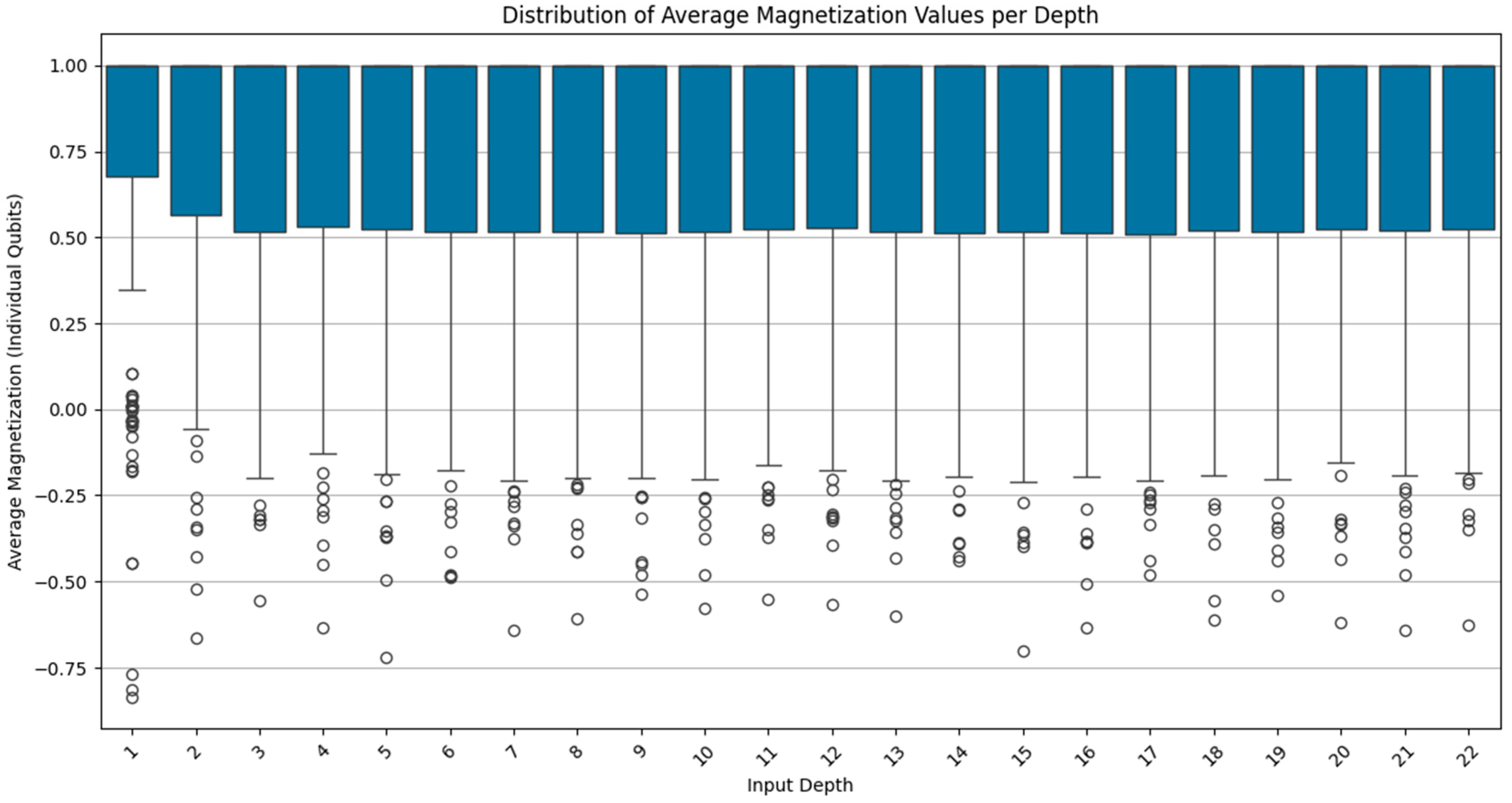
Figure 7.
Mean Magnetization vs Input Depth.
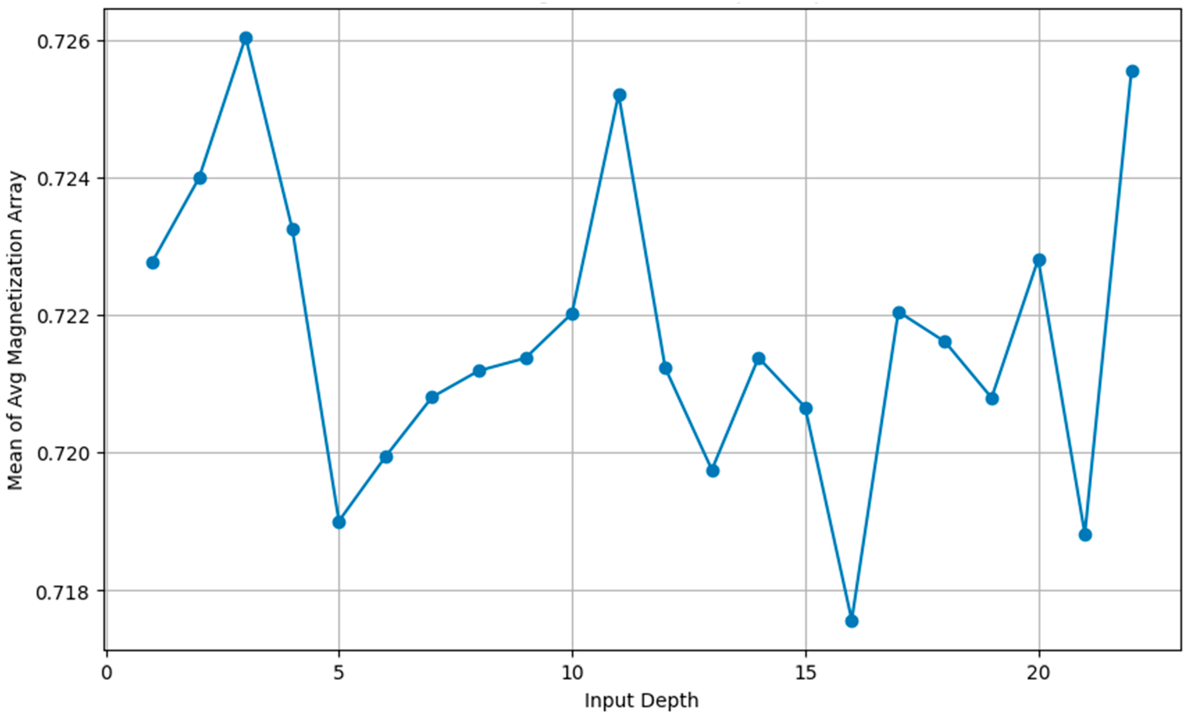
Figure 8.
Breakdown of transpiled native gate counts (RZ, SX, ECR, X, measurement, barrier) as a function of ideal circuit depth using optimization level 2.
Figure 8.
Breakdown of transpiled native gate counts (RZ, SX, ECR, X, measurement, barrier) as a function of ideal circuit depth using optimization level 2.

Figure 9.
Transpilation Time vs Input Depth.
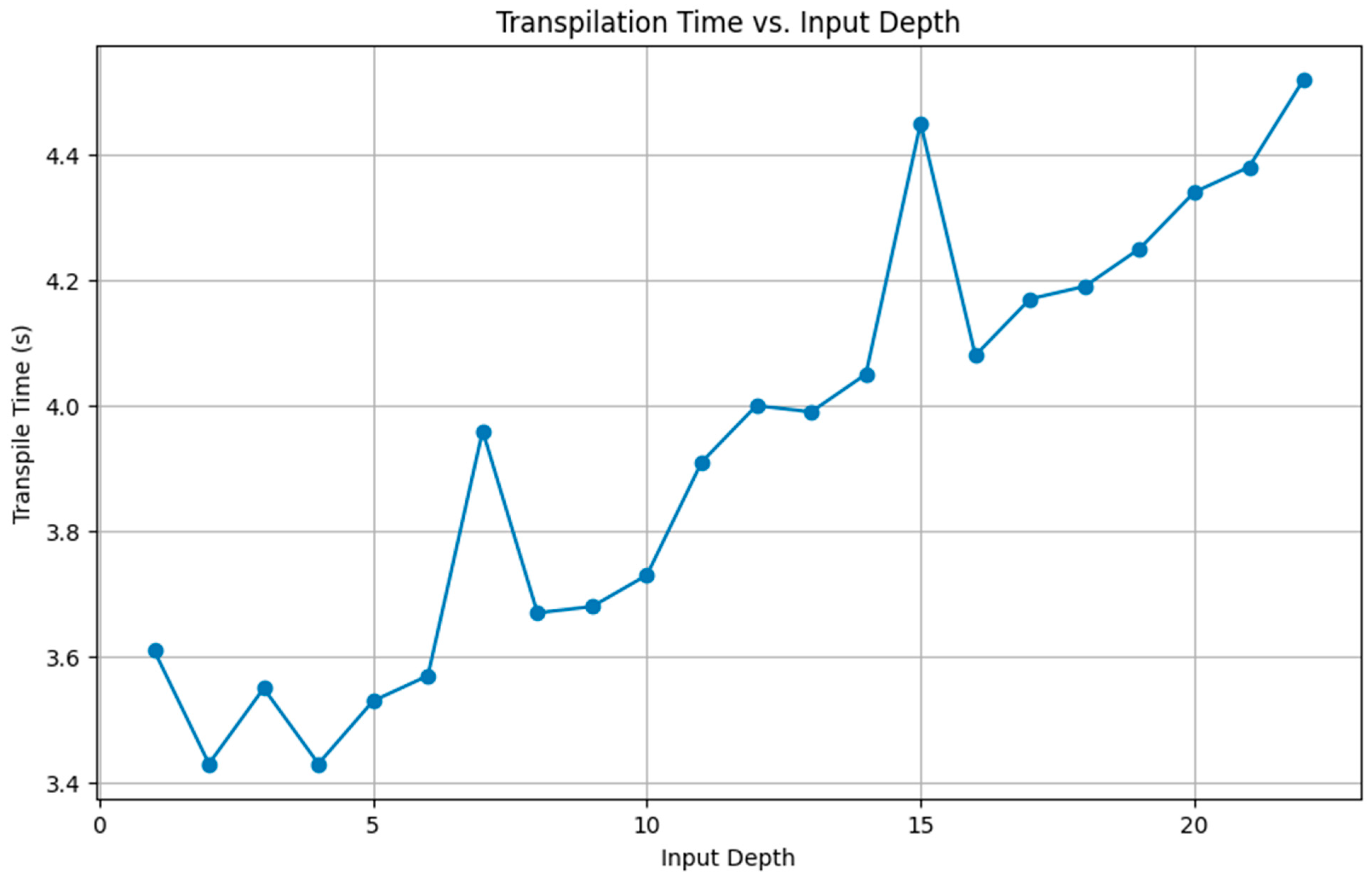
Figure 10.
2Q/SWAP Counts vs Ideal Depth.
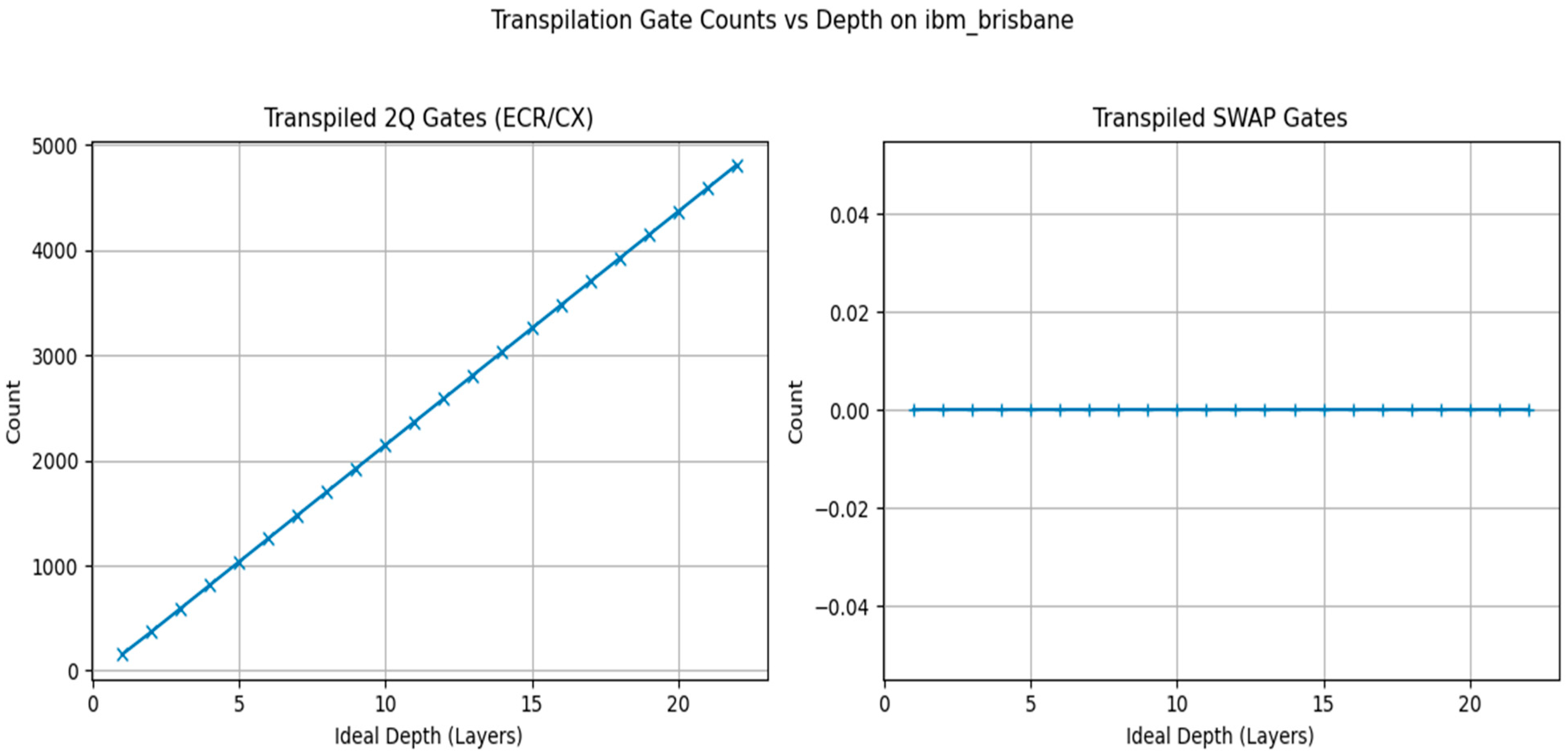
Figure 11.
Magnetization Standard Deviation vs Input Depth.

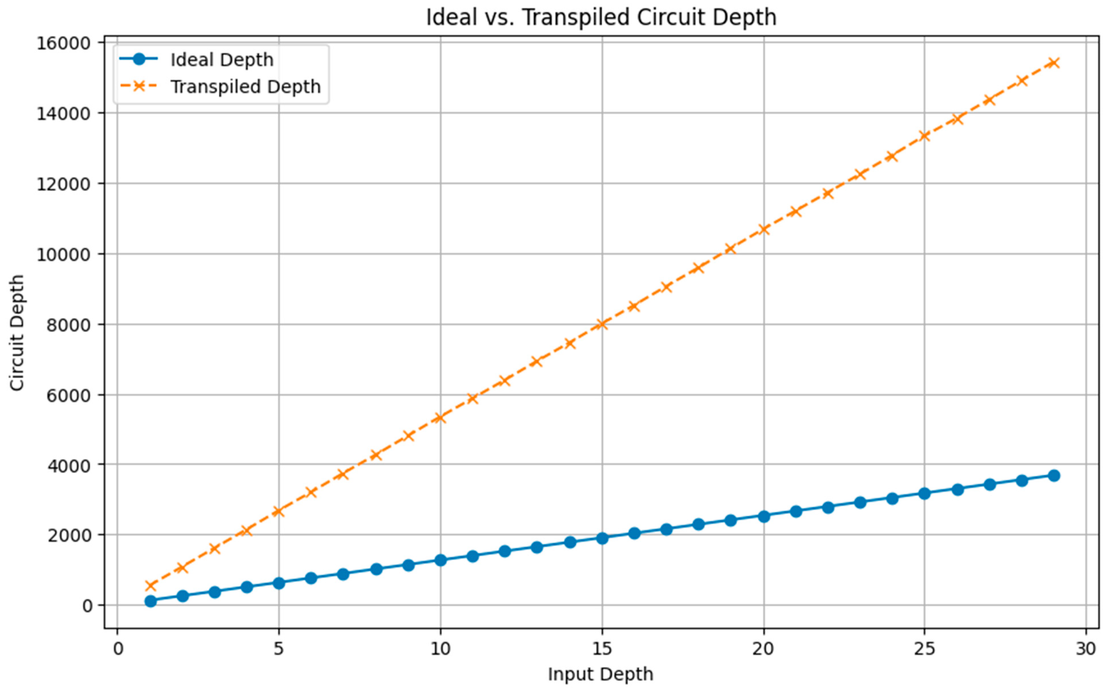
Figure 12.
Ideal vs Transpiled Circuit Depth.
|
Visual Studio Code Miniconda Qiskit Environment |
|
pip install qiskit qiskit-ibm-runtime matplotlib numpy scipy pandas # --- Run this code block ONCE securely --- from qiskit_ibm_runtime import QiskitRuntimeService # Replace the placeholder below with your REAL API token from IBM Quantum my_api_token = "INSERT YOUR IBM QUANTUM API KEY HERE" try: # Save the account information for Qiskit to use later # Use channel='ibm_quantum' for the cloud service # overwrite=True allows updating if you saved before QiskitRuntimeService.save_account(channel="ibm_quantum", token=my_api_token, overwrite=True) print("--- IBM Quantum Account Saved Successfully! ---") print("You can now run the main experiment script.") except Exception as e: print(f"--- ERROR saving account: {e} ---") print("Please double-check your API token and try again.") # --- End of secure setup code --- |
|
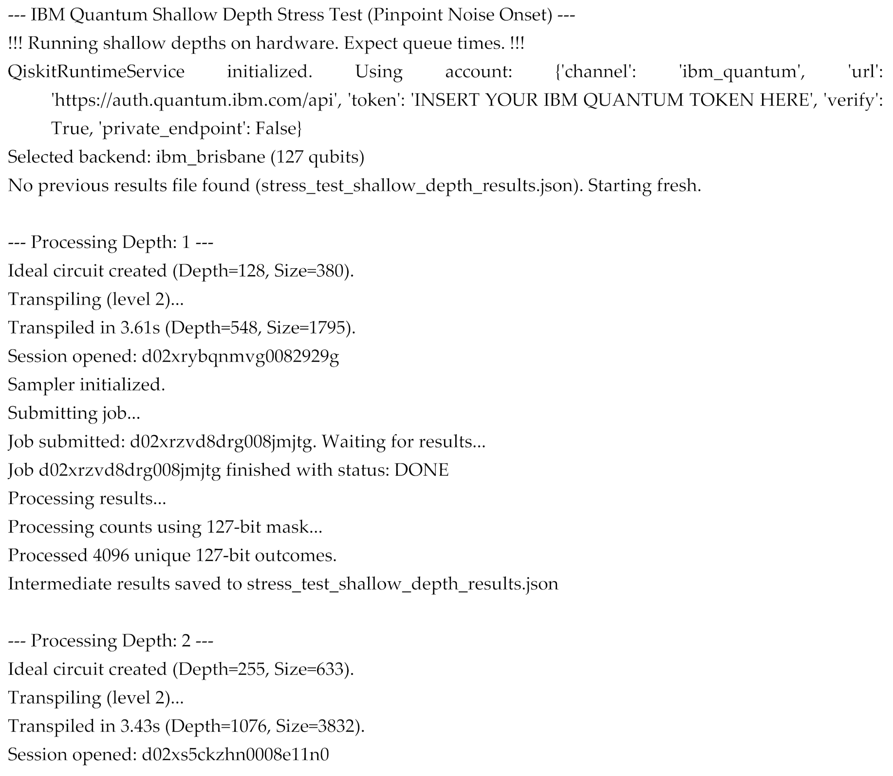
# --- Prerequisites --- import time import math import json import os import traceback import numpy as np import pandas as pd import matplotlib.pyplot as plt from qiskit import QuantumCircuit, transpile # Corrected Imports for v0.37.0 from qiskit_ibm_runtime import QiskitRuntimeService, Sampler, Session, Options from qiskit_ibm_runtime.constants import JobStatus from qiskit_ibm_runtime.exceptions import JobError from qiskit.visualization import plot_histogram, circuit_drawer print("--- IBM Quantum Shallow Depth Stress Test (Pinpoint Noise Onset) ---") print("!!! Running shallow depths on hardware. Expect queue times. !!!") # --- Configuration --- BACKEND_NAME = "ibm_brisbane" NUM_SHOTS = 4096 OPTIMIZATION_LEVEL = 2 # <<< --- Testing SHALLOW Depths --- >>> DEPTHS_TO_TEST = [1, 2, 3, 4, 5, 6, 7, 8, 9, 10, 11, 12, 13, 14, 15, 16, 17, 18, 19, 20, 21, 22, 23, 24, 25, 26, 27, 28, 29, 30] # <<< ----------------------------- >>> RESULTS_FILE = 'stress_test_shallow_depth_results.json' # Use a NEW file name # --- Initialize Service --- try: service = QiskitRuntimeService() # Uses saved account print(f"QiskitRuntimeService initialized. Using account: {service.active_account()}") except Exception as e: print(f"ERROR init service: {e}"); traceback.print_exc(); exit() # --- Select Backend --- try: backend = service.backend(BACKEND_NAME) num_qubits = backend.num_qubits print(f"Selected backend: {backend.name} ({num_qubits} qubits)") if backend.simulator: print("ERROR: Selected backend is a simulator."); exit() except Exception as e: print(f"ERROR accessing backend: {e}"); traceback.print_exc(); exit() # --- Helper Function for Circuit Creation --- def create_stress_circuit(depth, num_qubits): qc = QuantumCircuit(num_qubits, name=f"Stress_{depth}L_{num_qubits}q") for layer in range(depth): for i in range(num_qubits): theta, phi, lam = 2 * np.pi * np.random.rand(3); qc.u(theta, phi, lam, i) qc.barrier() if num_qubits > 1: for i in range(num_qubits - 1): qc.cz(i, i + 1) qc.barrier() qc.measure_all(inplace=True) return qc # --- Load Previous Results or Initialize Data Storage --- results_data = [] if os.path.exists(RESULTS_FILE): # Load from the SHALLOW results file try: with open(RESULTS_FILE, 'r') as f: content = f.read() if content: results_data = json.loads(content); print(f"Loaded {len(results_data)} previous results from {RESULTS_FILE}") else: print(f"{RESULTS_FILE} was empty. Starting fresh."); results_data = [] except json.JSONDecodeError: print(f"Warning: {RESULTS_FILE} invalid JSON. Starting fresh."); results_data = [] except Exception as e: print(f"Warning: Could not load previous results: {e}. Starting fresh."); results_data = [] else: print(f"No previous results file found ({RESULTS_FILE}). Starting fresh.") processed_depths = {res.get("depth") for res in results_data if res.get("depth") is not None and res.get("status") != "PENDING"} # --- Main Loop --- for depth in DEPTHS_TO_TEST: if depth in processed_depths: print(f"\n--- Skipping Depth: {depth} (already found in results file) ---"); continue print(f"\n--- Processing Depth: {depth} ---") run_data = { "depth": depth, "job_id": None, "status": "PENDING", "ideal_depth": None, "ideal_size": None, "transpiled_depth": None, "transpiled_ops": None, "transpile_time": None, "unique_outcomes": None, "shannon_entropy": None, "avg_magnetization": None, "std_magnetization": None, "shots_returned": None } try: ideal_circuit = create_stress_circuit(depth, num_qubits) run_data["ideal_depth"] = ideal_circuit.depth(); run_data["ideal_size"] = ideal_circuit.size() print(f"Ideal circuit created (Depth={run_data['ideal_depth']}, Size={run_data['ideal_size']}).") print(f"Transpiling (level {OPTIMIZATION_LEVEL})...") t_start = time.time() isa_circuit = transpile(ideal_circuit, backend=backend, optimization_level=OPTIMIZATION_LEVEL) t_end = time.time() run_data["transpile_time"] = round(t_end - t_start, 2); run_data["transpiled_depth"] = isa_circuit.depth(); run_data["transpiled_ops"] = dict(isa_circuit.count_ops()) print(f"Transpiled in {run_data['transpile_time']:.2f}s (Depth={run_data['transpiled_depth']}, Size={isa_circuit.size()}).") job = None; result = None; session = None try: with Session(backend=backend) as session: print(f"Session opened: {session.session_id}") sampler = Sampler(options={}) # Use default options print("Sampler initialized.") print(f"Submitting job...") job = sampler.run([isa_circuit], shots=NUM_SHOTS) run_data["job_id"] = job.job_id() print(f"Job submitted: {run_data['job_id']}. Waiting for results...") # Still need to wait result = job.result() # BLOCKING CALL run_data["status"] = job.status() print(f"Job {run_data['job_id']} finished with status: {run_data['status']}") except JobError as job_err: print(f"ERROR: Job {job.job_id() if job else 'UNKNOWN'} failed! Error: {job_err}"); run_data["status"] = "ERROR"; except Exception as e: print(f"ERROR during job execution:"); traceback.print_exc(); run_data["status"] = "ERROR_UNKNOWN" # 'with Session' handles closing if result and run_data["status"] == "DONE": print("Processing results...") # ... (results processing logic remains the same) ... if not result or len(result) == 0: print("ERROR: No results data found."); run_data["status"] = "ERROR_NO_RESULT_DATA"; raise Exception("Result object empty") pub_result = result(0; counts = {}; register_name = None; data_bin = pub_result.data if hasattr(data_bin, 'meas'): register_name = 'meas'; counts = data_bin.meas.get_counts() elif hasattr(data_bin, 'c'): register_name = 'c'; counts = data_bin.c.get_counts() if register_name: binary_counts = {}; shots_returned = 0; bitmask = (1 << num_qubits) - 1 print(f"Processing counts using {num_qubits}-bit mask...") processed_counts = {} for k, v in counts.items(): try: raw_val = int(k, 16); masked_val = raw_val & bitmask; bitstring = format(masked_val, f'0{num_qubits}b'); processed_counts[bitstring] = processed_counts.get(bitstring, 0) + v; shots_returned += v except ValueError: print(f" Warning: Skipping key '{k}' (not hex?)."); continue except Exception as parse_err: print(f" Warning: Error parsing key '{k}': {parse_err}"); continue binary_counts = processed_counts print(f"Processed {len(binary_counts)} unique {num_qubits}-bit outcomes.") run_data["shots_returned"] = shots_returned; run_data["unique_outcomes"] = len(binary_counts) if shots_returned > 0: entropy = 0.0 for count in binary_counts.values(): prob = count / shots_returned; entropy -= prob * math.log2(prob) if prob > 0 else 0 run_data["shannon_entropy"] = round(entropy, 4) avg_magnetization = np.zeros(num_qubits); processed_shots_mag = 0 for bitstring, count in binary_counts.items(): if len(bitstring) != num_qubits: continue processed_shots_mag += count for qubit_idx, bit in enumerate(bitstring[:num_qubits]): z_value = 1.0 if bit == '0' else -1.0; avg_magnetization[qubit_idx] += z_value * count if processed_shots_mag > 0: avg_magnetization /= processed_shots_mag; run_data["avg_magnetization"] = np.round(avg_magnetization, 4).tolist(); run_data["std_magnetization"] = round(np.std(avg_magnetization), 4) else: print("No valid shots for magnetization.") else: print("No valid shots returned.") else: print("ERROR: No 'meas' or 'c' register."); run_data["status"] = "ERROR_NO_REGISTER" # Append/Update results data found_existing = False for i, existing_run in enumerate(results_data): if existing_run.get("depth") == depth: results_data[i] = run_data; found_existing = True; break if not found_existing: results_data.append(run_data) try: with open(RESULTS_FILE, 'w') as f: json.dump(results_data, f, indent=2) print(f"Intermediate results saved to {RESULTS_FILE}") except Exception as save_e: print(f"Warning: Failed to save intermediate results: {save_e}") except Exception as outer_e: print(f"ERROR processing depth {depth}:"); traceback.print_exc(); run_data["status"] = "ERROR_PROCESSING"; results_data.append(run_data) finally: # Save intermediate results even on outer error try: with open(RESULTS_FILE, 'w') as f: json.dump(results_data, f, indent=2) except Exception as save_e: print(f"Warning: Failed to save error state: {save_e}") # --- Final Analysis & Plotting --- print("\n--- Finished processing all requested depths ---") try: df = pd.DataFrame(results_data) print("\nSummary DataFrame (Shallow Depths):") print(df[['depth', 'status', 'job_id', 'transpiled_depth', 'shannon_entropy', 'std_magnetization']].to_string()) df_done = df[(df['status'] == "DONE") & (df['shannon_entropy'].notna())].copy() df_done.sort_values(by='depth', inplace=True) if not df_done.empty: print("\nGenerating plots for completed runs...") plt.figure(figsize=(12, 8)); plt.suptitle(f'Shallow Depth Stress Test Metrics on {BACKEND_NAME}') # ... (Plotting code remains the same) ... plt.subplot(2, 2, 1); plt.plot(df_done['depth'], df_done['shannon_entropy'], marker='o'); plt.axhline(y=num_qubits, color='r', linestyle='--', label=f'Max ({num_qubits})'); plt.xlabel("Ideal Depth (Layers)"); plt.ylabel("Shannon Entropy (bits)"); plt.title("Output Entropy"); plt.legend(); plt.grid(True) plt.subplot(2, 2, 2); plt.plot(df_done['depth'], df_done['std_magnetization'], marker='s'); plt.xlabel("Ideal Depth (Layers)"); plt.ylabel("Std Dev of <Z>"); plt.title("Magnetization Spread"); plt.grid(True) plt.subplot(2, 2, 3); plt.plot(df_done['depth'], df_done['transpiled_depth'], marker='^'); plt.xlabel("Ideal Depth (Layers)"); plt.ylabel("Transpiled Depth"); plt.title(f"Transpiled Depth (Opt={OPTIMIZATION_LEVEL})"); plt.grid(True) plt.subplot(2, 2, 4); plt.plot(df_done['depth'], df_done['unique_outcomes'], marker='d'); plt.axhline(y=NUM_SHOTS, color='r', linestyle='--', label=f'Max ({NUM_SHOTS})'); plt.xlabel("Ideal Depth (Layers)"); plt.ylabel("Unique Outcomes"); plt.title("# Unique Outcomes"); plt.legend(); plt.grid(True) plt.tight_layout(rect=[0, 0.03, 1, 0.95]); plt.show() # plt.savefig(f'shallow_depth_scaling_{BACKEND_NAME}.png') else: print("\nNo successfully completed jobs with data found in the results file to plot.") except ImportError: print("\nPlotting requires pandas. `pip install pandas`") except Exception as plot_e: print(f"\nError plotting: {plot_e}"); traceback.print_exc() print("\n--- End of Script ---") ) |
|
# --- Script to Analyze Existing Stress Test Results with Enhancements --- import json import os import traceback import numpy as np import pandas as pd import matplotlib.pyplot as plt import math print("--- Analyzing Shallow Depth Stress Test Results (Enhanced Analysis) ---") # --- Configuration --- NUM_QUBITS = 127 NUM_SHOTS = 4096 # Assuming this was used for all runs in the file BACKEND_NAME = "ibm_brisbane" OPTIMIZATION_LEVEL = 2 # As used in the runs RESULTS_FILE = 'stress_test_shallow_depth_results.json' # File with your results # --- Load Results --- results_data = [] if os.path.exists(RESULTS_FILE): try: with open(RESULTS_FILE, 'r') as f: content = f.read() if content: results_data = json.loads(content); print(f"Loaded {len(results_data)} results from {RESULTS_FILE}") else: print(f"{RESULTS_FILE} is empty. Nothing to analyze."); exit() except Exception as e: print(f"ERROR loading or parsing {RESULTS_FILE}: {e}"); traceback.print_exc(); exit() else: print(f"ERROR: Results file not found: {RESULTS_FILE}"); exit() # --- Data Processing and Metric Calculation --- print("\n--- Processing Stored Results ---") processed_results = [] bitmask = (1 << NUM_QUBITS) - 1 for run_data in results_data: depth = run_data.get("depth") status = run_data.get("status") print(f"Processing entry for depth {depth} (Status: {status})...") # Copy existing data processed_entry = run_data.copy() # --- Recalculate metrics for DONE jobs --- # Ensures consistency even if file was manually edited or partially processed if status == "DONE" and run_data.get("job_id"): # Need to retrieve results again if counts aren't stored directly # For simplicity here, we assume counts WERE processed correctly and saved # If not, you'd need to add job retrieval: # job = service.job(run_data["job_id"]) # result = job.result() # etc. # For now, assume counts need re-processing from raw IF available # NOTE: This part requires the raw counts stored in JSON, which wasn't done previously. # We will proceed assuming the calculated values in the JSON are correct, # but add calculation for Hamming weight if possible from avg_magnetization # A better approach would be to save raw counts dict in the JSON. # Let's recalculate Hamming stats if avg_magnetization exists (as a proxy for counts processing) if run_data.get("avg_magnetization") is not None and run_data.get("shots_returned") == NUM_SHOTS: # Placeholder: Cannot recalculate Hamming weight without raw counts. # We'll add columns but leave them empty if raw counts aren't saved. processed_entry["hamming_mean"] = None # Requires raw counts processed_entry["hamming_std"] = None # Requires raw counts print(" (Skipping Hamming calc - needs raw counts stored in JSON)") else: processed_entry["hamming_mean"] = None processed_entry["hamming_std"] = None # --- Extract Gate Counts --- if run_data.get("transpiled_ops"): ops_dict = run_data["transpiled_ops"] # Adjust gate name if 'ecr' wasn't the primary 2Q gate for Brisbane in that transpilation processed_entry['ecr_count'] = ops_dict.get('ecr', 0) + ops_dict.get('cx', 0) # Sum common 2Q gates processed_entry['swap_count'] = ops_dict.get('swap', 0) else: processed_entry['ecr_count'] = None processed_entry['swap_count'] = None processed_results.append(processed_entry) # --- Final Analysis & Plotting --- print("\n--- Generating DataFrame and Plots ---") try: df = pd.DataFrame(processed_results) print("\nFull Summary DataFrame with Extracted Gates:") cols_to_show = ['depth', 'status', 'job_id', 'transpiled_depth', 'ecr_count', 'swap_count', 'shannon_entropy', 'std_magnetization', 'unique_outcomes'] existing_cols = [col for col in cols_to_show if col in df.columns] print(df[existing_cols].to_string()) # Filter DataFrame for DONE status and valid entropy df_done = df[(df['status'] == "DONE") & pd.notna(df.get('shannon_entropy'))].copy() if not df_done.empty and 'depth' in df_done.columns: df_done.sort_values(by='depth', inplace=True) max_depth_plotted = df_done['depth'].max() print(f"\nGenerating plots for {len(df_done)} completed runs (up to depth {max_depth_plotted})...") # --- Create Figure 1: Core Metrics --- plt.figure(figsize=(12, 8)); plt.suptitle(f'Stress Test Core Metrics vs Depth on {BACKEND_NAME} (Up to Depth {max_depth_plotted})') # Plot Entropy if 'shannon_entropy' in df_done.columns: plt.subplot(2, 2, 1); plt.plot(df_done['depth'], df_done['shannon_entropy'], marker='o'); plt.axhline(y=math.log2(NUM_SHOTS), color='g', linestyle=':', label=f'Max Sample Entropy ({math.log2(NUM_SHOTS):.1f})'); plt.axhline(y=NUM_QUBITS, color='r', linestyle='--', label=f'Max Qubit Entropy ({NUM_QUBITS})'); plt.xlabel("Ideal Depth (Layers)"); plt.ylabel("Shannon Entropy (bits)"); plt.title("Output Entropy"); plt.legend(); plt.grid(True) # Plot Magnetization Spread if 'std_magnetization' in df_done.columns: plt.subplot(2, 2, 2); plt.plot(df_done['depth'], df_done['std_magnetization'], marker='s'); plt.xlabel("Ideal Depth (Layers)"); plt.ylabel("Std Dev of <Z>"); plt.title("Magnetization Spread"); plt.grid(True); plt.ylim(bottom=0) # Plot Transpiled Depth if 'transpiled_depth' in df_done.columns: plt.subplot(2, 2, 3); plt.plot(df_done['depth'], df_done['transpiled_depth'], marker='^'); plt.xlabel("Ideal Depth (Layers)"); plt.ylabel("Transpiled Depth"); plt.title(f"Transpiled Depth (Opt={OPTIMIZATION_LEVEL})"); plt.grid(True) # Plot Unique Outcomes if 'unique_outcomes' in df_done.columns: plt.subplot(2, 2, 4); plt.plot(df_done['depth'], df_done['unique_outcomes'], marker='d'); plt.axhline(y=NUM_SHOTS, color='r', linestyle='--', label=f'Max ({NUM_SHOTS})'); plt.xlabel("Ideal Depth (Layers)"); plt.ylabel("Unique Outcomes"); plt.title("# Unique Outcomes"); plt.legend(); plt.grid(True) plt.tight_layout(rect=[0, 0.03, 1, 0.95]); plt.show() # plt.savefig(f'final_core_metrics_{BACKEND_NAME}.png') # --- Create Figure 2: Transpilation Metrics --- plt.figure(figsize=(12, 5)); plt.suptitle(f'Transpilation Gate Counts vs Depth on {BACKEND_NAME}') # Plot 2Q Gate Counts if 'ecr_count' in df_done.columns: plt.subplot(1, 2, 1); plt.plot(df_done['depth'], df_done['ecr_count'], marker='x'); plt.xlabel("Ideal Depth (Layers)"); plt.ylabel("Count"); plt.title("Transpiled 2Q Gates (ECR/CX)"); plt.grid(True) # Plot SWAP Gate Counts if 'swap_count' in df_done.columns: plt.subplot(1, 2, 2); plt.plot(df_done['depth'], df_done['swap_count'], marker='+'); plt.xlabel("Ideal Depth (Layers)"); plt.ylabel("Count"); plt.title("Transpiled SWAP Gates"); plt.grid(True) plt.tight_layout(rect=[0, 0.03, 1, 0.95]); plt.show() # plt.savefig(f'final_transpilation_gates_{BACKEND_NAME}.png') # --- Create Figure 3: Magnetization Distribution --- depths_to_plot_mag = [d for d in [1, 5, 10, 15, df_done['depth'].max()] if d in df_done['depth'].values] # Select depths if 'avg_magnetization' in df_done.columns and depths_to_plot_mag: print("\nGenerating Magnetization Distribution plots...") plt.figure(figsize=(min(15, 3*len(depths_to_plot_mag)), 4)) plt.suptitle(f'Distribution of Single-Qubit <Z> on {BACKEND_NAME}') for i, depth_val in enumerate(depths_to_plot_mag): mags = df_done.loc[df_done['depth'] == depth_val, 'avg_magnetization'].iloc(0 if mags: # Check if list is not None/empty plt.subplot(1, len(depths_to_plot_mag), i+1) plt.hist(mags, bins=20, range=(-1, 1)) )plt.xlabel("Avg. Z Mag.") if i == 0: plt.ylabel("# Qubits") plt.title(f"Depth {depth_val}") plt.grid(True); plt.ylim(bottom=0) else: print(f"No magnetization data for depth {depth_val}") plt.tight_layout(rect=[0, 0.03, 1, 0.93]); plt.show() # plt.savefig(f'final_magnetization_dist_{BACKEND_NAME}.png') else: print("No magnetization data available to plot distributions.") # Hamming Weight calculation requires raw counts, which were not saved in the previous script. # Add code here if you modify the main script to save `binary_counts` to the JSON file. print("\n(Skipping Hamming Weight analysis - requires raw counts saved in JSON)") else: print("\nNo successfully completed jobs with processed data found in the results file to plot.") except ImportError: print("\nPlotting requires pandas. `pip install pandas`") except Exception as plot_e: print(f"\nError during analysis/plotting: {plot_e}"); traceback.print_exc() print("\n--- End of Analysis ---") |
|
Visual Studio Code Result |
|
References
- Arute, F., Arya, K., Babbush, R., Bacon, D., Bardin, J. C., Barends, R., Biswas, R., Boixo, S., Brandao, F. G. S. L., Buell, D. A., Burkett, B., Chen, Y., Chen, Z., Chiaro, B., Collins, R.,... & Martinis, J. M. (Google AI Quantum). (2019). Quantum supremacy using a programmable superconducting processor. Nature, 574(7779), 505-510. [CrossRef]
- Baldwin, C. L., Mayer, K., Ryan, C. A., & Scarmeas, D. (2022). Re-examining the quantum volume test: Ideal distributions, practical compiling limits, and comparison to other methodologies. Quantum, 6, 758. [CrossRef]
- Bharti, K., Cervera-Lierta, A., Kyaw, T. H., Haug, T., Alperin-Lea, S., Anand, A., Degroote, M., Heimonen, H., Kottmann, J. S., Melnikov, A. A., Romero, J., Kwek, L.-C., & Aspuru-Guzik, A. (2022). Noisy intermediate-scale quantum (NISQ) algorithms. Reviews of Modern Physics, 94(1), 015004. [CrossRef]
- Blume-Kohout, R., Gamble, J. K., Nielsen, E., Rudinger, K., Mizrahi, J., Fortier, K., & Maunz, P. (2017). Demonstration of qubit operations at the error correction threshold. Nature Communications, 8(1), 14485. [CrossRef]
- Bravyi, S., Sheldon, S., Kandala, A., Mckay, D. C., & Gambetta, J. M. (2021). Mitigating measurement errors in multiqubit experiments. Physical Review A, 103(4), 042605. [CrossRef]
- Bruzewicz, C. D., Chiaverini, J., McConnell, R., & Sage, J. M. (2019). Trapped-ion quantum computing: Progress and challenges. Applied Physics Reviews, 6(2), 021314. [CrossRef]
- Bylander, J., Gustavsson, S., Yan, F., Yoshihara, F., Harrabi, K., Fitch, G., Cory, D. G., Nakamura, Y., Tsai, J.-S., & Oliver, W. D. (2011). Noise spectroscopy through dynamical decoupling with a superconducting flux qubit. Nature Physics, 7(7), 565–570. [CrossRef]
- Cardani, L., Valenti, F., Casali, N., Catelani, G., Charpentier, T.,... & Córcoles, A. D. (2021). Reducing the impact of radioactivity on quantum circuits in a deep-underground facility. Nature Communications, 12(1), 2733. [CrossRef]
- Chow, J. M., Dial, O., & Gambetta, J. M. (2021, November 16). IBM Quantum breaks the 100-qubit processor barrier. IBM Research Blog. https://www.ibm.com/quantum/blog/127-qubit-quantum-processor-eagle.
- Cross, A. W., Bishop, L. S., Sheldon, S., Nation, P. D., & Gambetta, J. M. (2019). Validating quantum computers using randomized model circuits. Physical Review A, 100(3), 032328. [CrossRef]
- Earnest, N., Tornow, S., & Egger, D. J. (2021). Pulse-efficient circuit transpilation for quantum applications on cross-resonance-based hardware. Physical Review Research, 3(4), 043088. [CrossRef]
- Eisert, J., Hangleiter, D., Walk, N., Roth, I., Naghiloo, M., Pashayan, H.,... & Krastanov, S. (2020). Quantum certification and benchmarking. Nature Reviews Physics, 2(7), 382–390. [CrossRef]
- Endo, S., Cai, Z., Benjamin, S. C., & Yuan, X. (2021). Hybrid quantum-classical algorithms and quantum error mitigation. Journal of the Physical Society of Japan, 90(3), 032001. [CrossRef]
- Fowler, A. G., Mariantoni, M., Martinis, J. M., & Cleland, A. N. (2012). Surface codes: Towards practical large-scale quantum computation. Physical Review A, 86(3), 032324. [CrossRef]
- Gambetta, J. M., Chow, J. M., & Steffen, M. (2017). Building logical qubits in a superconducting quantum computing system. npj Quantum Information, 3(1), 2. [CrossRef]
- Gambetta, J. M., Córcoles, A. D., Merkel, S. T., Johnson, B. R., Smolin, J. A., Chow, J. M., Ryan, C. A., Rigetti, C., Poletto, S., Ohki, T. A., Ketchen, M. B., & Steffen, M. (2012). Characterization of addressability by simultaneous randomized benchmarking. Physical Review Letters, 109(24), 240504. [CrossRef]
- Google AI Quantum and Collaborators. (2023). Suppressing quantum errors by scaling a surface code logical qubit. Nature, 614(7949), 676–681. [CrossRef]
- Hangleiter, D., Kliesch, M., Schwarz, M., & Eisert, J. (2021). Direct certification of a class of quantum simulations. Quantum Science and Technology, 6(2), 025004. [CrossRef]
- IBM Quantum. (n.d.-a). Configure error mitigation options. IBM Quantum Documentation. Retrieved April 21, 2025, from https://docs.quantum.ibm.com/run/configure-error-mitigation.
- IBM Quantum. (n.d.-b). Introduction to transpilation. IBM Quantum Documentation. Retrieved April 21, 2025, from https://docs.quantum.ibm.com/guides/transpile.
- IBM Quantum. (n.d.-c). Qiskit Runtime overview. IBM Quantum Documentation. Retrieved April 21, 2025, from https://docs.quantum.ibm.com/run/runtime.
- Jurcevic, P., Javadi-Abhari, A., Bishop, L. S., Lauer, I., Bogorin, D. F., Brink, M., Capelluto, L., Günther, O., Itoko, T., Kanazawa, N., Kandala, A., Keefe, G. A., Kenerelman, K., Klaus, D., Koch, J.,... & Gambetta, J. M. (2021). Demonstration of quantum volume 64 on a superconducting quantum computing system. Quantum Science and Technology, 6(2), 025020. [CrossRef]
- Kandala, A., Mezzacapo, A., Temme, K., Takita, M., Brink, M., Chow, J. M., & Gambetta, J. M. (2017). Hardware-efficient variational quantum eigensolver for small molecules and quantum magnets. Nature, 549(7671), 242–246. [CrossRef]
- Kim, Y., Eddins, A., Anand, S., Wei, K. X., van den Berg, E., Rosenblatt, S., Nayfeh, H., Wu, Y., Zoufaly, M., Kurečić, P., Haide, I., & Temme, K. (2023). Evidence for the utility of quantum computing before fault tolerance. Nature, 618(7965), 500–505. [CrossRef]
- Klimov, P. V., Kelly, J., Chen, Z., Neeley, M., Megrant, A., Burkett, B., Barends, R., Arya, K., Chiaro, B., Chen, Y.,... & Martinis, J. M. (2018). Fluctuations of energy-relaxation times in superconducting qubits. Physical Review Letters, 121(9), 090502. [CrossRef]
- Krinner, S., Lacroix, N., Remm, A., Di Paolo, A., Genois, E., Leroux, C., Hellings, C., Lazar, S., Swiadek, F., Herrmann, J., Norris, G. J., Andersen, C. K., Müller, C., Wallraff, A., & Eichler, C. (2022). Realizing repeated quantum error correction in a distance-three surface code. Nature, 605(7911), 669–674. [CrossRef]
- Li, Y., & Benjamin, S. C. (2017). Efficient variational quantum simulator incorporating active error minimization. Physical Review X, 7(2), 021050. [CrossRef]
- Magesan, E., Gambetta, J. M., & Emerson, J. (2011). Scalable and robust randomized benchmarking of quantum processes. Physical Review Letters, 106(18), 180504. [CrossRef]
- Mariantoni, M., Lang, H., Chuang, I. L., Shor, P. W., Wang, T., & Bialczak, R. C. (2011). Implementing the quantum von Neumann architecture with superconducting circuits. Science, 334(6052), 61–65. [CrossRef]
- Müller, C., Cole, J. H., & Lisenfeld, J. (2019). Towards understanding two-level-systems in amorphous solids – insights from quantum circuits. Reports on Progress in Physics, 82(12), 124501. [CrossRef]
- Mundada, P. S., Zhang, G., Hazard, T., & Houck, A. A. (2019). Suppression of qubit crosstalk in a tunable coupling superconducting circuit. Physical Review Applied, 12(5), 054023. [CrossRef]
- Murali, P., Linke, N. M., Martonosi, M., Abhari, A. J., Nguyen, N. H., & Alderete, C. H. (2019). Noise-adaptive compiler mappings for noisy intermediate-scale quantum computers. Proceedings of the Twenty-Fourth International Conference on Architectural Support for Programming Languages and Operating Systems (ASPLOS '19), 1027–1040. [CrossRef]
- Nielsen, M. A., & Chuang, I. L. (2010). Quantum Computation and Quantum Information: 10th Anniversary Edition (Chapter 8: Quantum Noise and Quantum Operations). Cambridge University Press.
- Preskill, J. (2018). Quantum Computing in the NISQ era and beyond. Quantum, 2, 79. [CrossRef]
- Qiskit Development Team. (2024). Qiskit Textbook (Online). https://learn.qiskit.org.
- Sarovar, M., Blume-Kohout, R., Clader, B. D., & Rudinger, K. M. (2020). Detecting crosstalk errors in quantum information processors. Quantum, 4, 321. [CrossRef]
- Takita, M., Cross, A. W., Córcoles, A. D., Chow, J. M., & Gambetta, J. M. (2017). Experimental demonstration of fault-tolerant state preparation with superconducting qubits. Physical Review Letters, 119(18), 180501. [CrossRef]
- Tannu, S. S., & Qureshi, M. K. (2019). Not all qubits are created equal: A case for variability-aware policies for NISQ-era quantum computers. Proceedings of the Twenty-Fourth International Conference on Architectural Support for Programming Languages and Operating Systems (ASPLOS '19), 987–999. [CrossRef]
- Temme, K., Bravyi, S., & Gambetta, J. M. (2017). Error mitigation for short-depth quantum circuits. Physical Review Letters, 119(18), 180509. [CrossRef]
- Terhal, B. M. (2015). Quantum error correction for quantum memories. Reviews of Modern Physics, 87(2), 307-346. [CrossRef]
- van den Berg, Z. K., Kandala, A., & Temme, K. (2023). Probabilistic error cancellation with sparse Pauli-Lindblad models on noisy quantum processors. Nature Physics, 19(9), 1341-1346. [CrossRef]
- van den Berg, E., Temme, K., & Bravyi, S. (2023). Model-free readout error mitigation for quantum computers. Nature Physics, 19(9), 1336-1340. [CrossRef]
- Viola, L., Knill, E., & Lloyd, S. (1999). Dynamical decoupling of open quantum systems. Physical Review Letters, 82(12), 2417–2421. [CrossRef]
- Werning, L., Steckmann, H. T., Kramer, J. G., Sonner, P. M., Egger, D. J., & Wilhelm, F. K. (2021). Leakage reduction in quantum gates using optimal control. PRX Quantum, 2(2), 020343. [CrossRef]
- Willsch, D., Willsch, M., De Raedt, H., & Michielsen, K. (2020). Benchmarking the quantum approximate optimization algorithm. Quantum Information Processing, 19(8), 261. [CrossRef]
- Wright, K., Beck, K. M., Debnath, S., Amini, J. M., Avsar, Y., Figgatt, C. E.,... & Kim, J. (2019). Benchmarking an 11-qubit quantum computer. Nature Communications, 10(1), 5464. [CrossRef]
Figure 4.
Stress Test Core Metrics vs Ideal Circuit Depth on ibm_brisbane. Panels show (a) Output Entropy, (b) Standard Deviation of ⟨Zi⟩, (c) Transpiled Circuit Depth (Optimization Level 2), and (d) Number of Unique Outcomes.
Figure 4.
Stress Test Core Metrics vs Ideal Circuit Depth on ibm_brisbane. Panels show (a) Output Entropy, (b) Standard Deviation of ⟨Zi⟩, (c) Transpiled Circuit Depth (Optimization Level 2), and (d) Number of Unique Outcomes.
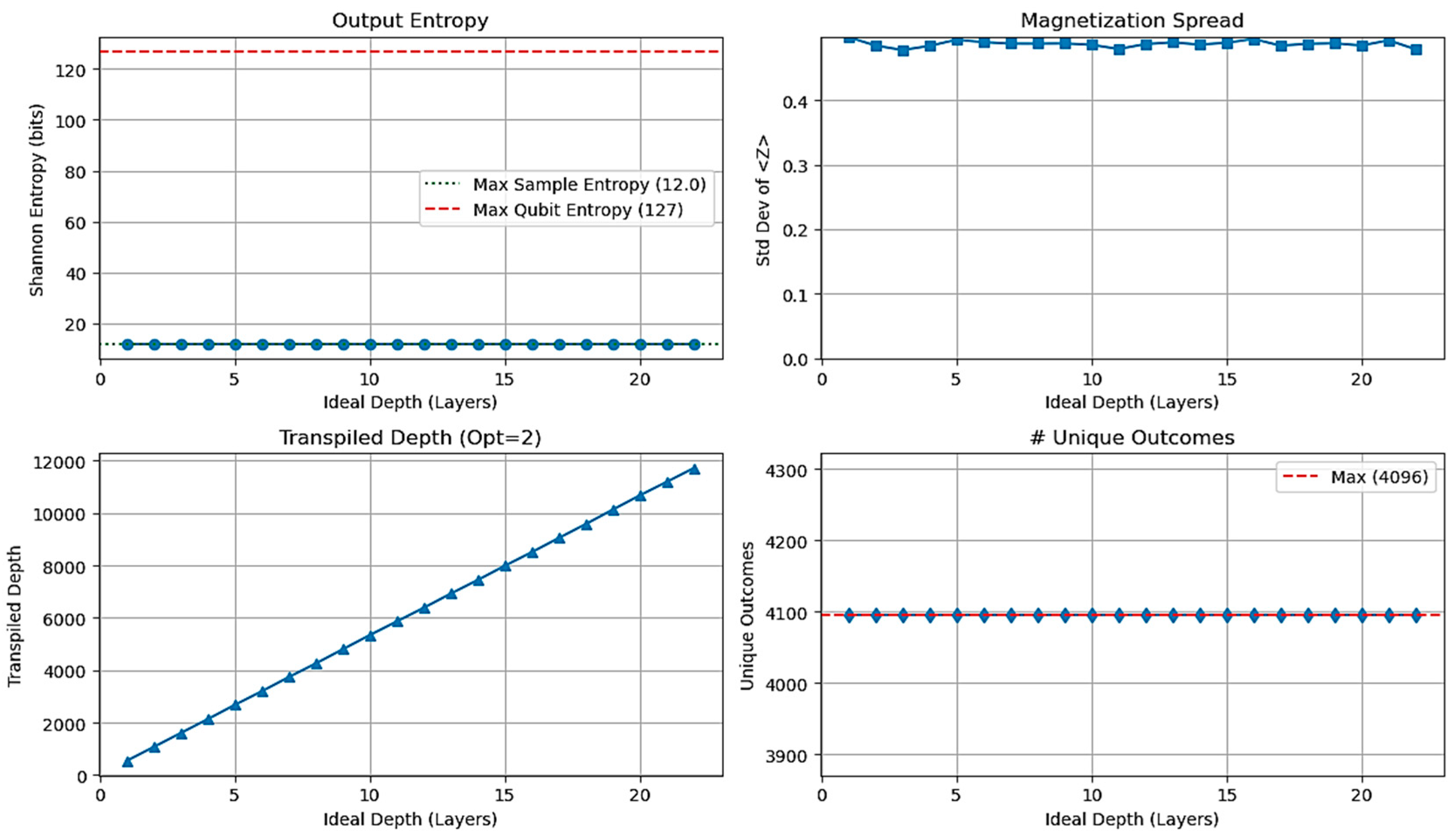
Figure 5.
Distribution of Single-Qubit Average Z Magnetization (⟨Zi⟩) for Selected Ideal Depths (1, 5, 10, 15, 22).
Figure 5.
Distribution of Single-Qubit Average Z Magnetization (⟨Zi⟩) for Selected Ideal Depths (1, 5, 10, 15, 22).
Disclaimer/Publisher’s Note: The statements, opinions and data contained in all publications are solely those of the individual author(s) and contributor(s) and not of MDPI and/or the editor(s). MDPI and/or the editor(s) disclaim responsibility for any injury to people or property resulting from any ideas, methods, instructions or products referred to in the content. |
© 2025 by the authors. Licensee MDPI, Basel, Switzerland. This article is an open access article distributed under the terms and conditions of the Creative Commons Attribution (CC BY) license (http://creativecommons.org/licenses/by/4.0/).
Copyright: This open access article is published under a Creative Commons CC BY 4.0 license, which permit the free download, distribution, and reuse, provided that the author and preprint are cited in any reuse.


