
Submitted:
15 April 2025
Posted:
16 April 2025
You are already at the latest version
Abstract
A novel approach to cosmic inflation within the framework of a non-commutative Riemannian foliated quantum gravity, built upon a reverse Faddeev–Jackiw symplectic spacetime deformation of the conventional Poisson algebra, is investigated. Friedmann-type dynamical equations, analitycally continued to a complex non-commutative framework, incorporate a modified energy-momentum Riemann tensor and a non-commutative matter-energy potential, highlighting the emergence of quantum gravity topological fluctuation effects on the expansion dynamics of the universe. In this realm, the coupling of UV and IR scales play a central role, providing a natural topological mechanism for inflation and recursal evidences for the generation of relic gravitational waves. These predictions align with a self-consistent description of the transition between the primordial mirror-universe deceleration and present-universe acceleration phases as predict by the Riemann foliated quantum gravity, offering potential connections to observational cosmology.
Keywords:
Quantum Gravity
; Branch Cut Cosmology
; Inflation
1. Introduction
A gauge field theory defined over a spacetime endowed with a noncommutative algebraic-geometric structure represents a relevant generalization of the standard structure of local quantum field theory, insofar as it explicitly emphasizes highly nontrivial and relevant physical aspects related to nonlocality.
A non-commutative geometry represents an extension of the conceptions that underlie standard geometry with respect to manifolds, metrics, and fiber bundles, insofar as the coordinates of space and time, which conventionally correspond to c-numbers, are replaced by operational fields.
A standard commutative geometry is replaced by a non-commutative Poisson-type symplectic algebraic structure of operators of the form
where the operators act in turn as generators of the algebraic structure, and where represents generalizations of structure constants for the ordinary Lie algebra.
In previous formulations [1,2], the path towards the non-commutative formulation was preceded by a commutative approach, based on the commutative projectable Hořava-Lifshitz gravity, which comprises an extension of general gravity that contemplates higher orders of the Ricci curvature scalar. The Einstein–Hilbert action, equipped with a Lorentzian signature () metric, corresponds to an integral in the four-dimensional spacetime manifold M, which produces Einstein field equations by means of the stationary action principle. The Einstein-Hilbert action is defined as
where represents the (negative) determinant of the Lorentzian spacetime metric tensor matrix; in this expression, R demotes the Ricci scalar curvature, G is the gravitational constant and c is the speed of light in vacuum.
The line element of the BCQG quantum gravity, resulting from the complexification of the FLRW metric [3,4,5,6], in tune with the ADM foliation [7], may be expressed as [8,9,10]
where , is a normalization constant, is the lapse function, represents the foliated scale factor as the result of the analytically continuation of the metric to the complex plane, and is the metric of the unit 3-sphere:
The commutative BCQG action depends on the branching scalar curvature of the universe, ,- an analytically continued counterpart of the Ricici scalar curvature R -, and on its covariant derivatives, , in different orders [1,2,11,12]:
The extrinsic curvature is given as
where represents the ADM shift vector and is the 3-dimensional covariant derivative. With the variable change , with , assuming the gauge , we obtain
where K represents the trace of .
2. Non-Commutative BCQG: Triad-Extended Formulation
Recently, based on an extended Faddeev–Jackiw deformation of the conventional Poisson algebra, we have developed an extension of Riemannian foliated branch-cut quantum gravity in a non-commutative symplectic spacetime domain (BCQG) [1,2]. This formulation allows to investigate non-commutativity effects as drivers of the cosmic expansion of the universe by means of a symplectic topological manifold spacetime structure that provides an isomorphic scenario composed of a triad of canonically conjugate scalar complex fields comprising complementary quantum dualities. The resulting extended manifold encompasses the canonical BCQG cosmic scale factor, , and its complementary quantum counterparts, outlined in the perfect Hermann Weyl fluid domain [13,14], . In addition, the extended manifold comprises an inflaton-type complex scalar field, , inspired by the original inflation model [15,16], resulting in the super-Hamiltonian (for the details, see [1,2]):
In this scenario, as emphasized earlier, the variables , and compose a triad of dual-conjugate complementary canonical quantum fields that shape an underlying non-commutative space-time structure. The running coupling constants in turn depict the primordial matter-energy configuration contributions of radiation (), baryon matter (), curvature (), quintessence (), cosmological constant dark energy (, and stiff matter () (for the details see [17,18] and references therein). Moreover, canonical quantization procedures applied to the Hamiltonian (7), allow the variables , and along with their corresponding conjugate momenta , , and to be treated as operators:
Combining equations (7) and (8) we obtain the following expression for the super-Hamiltonian:
In this formulation, chaotic inflation is modeled by the potential [15]
while for non-chaotic inflation, by the Fubini potential [19]
An important aspect to be punctuated is that, despite the adoption of an unconventional reverse mapping path for the Faddeev–Jackiw symplectic deformation of the conventional Poisson algebra, — which spawns a triad of commutative variables —, the above equation (7) embodies the effects of the reconfiguration of the originally commutative super-Hamiltonian by the imposition of a non-commutative symplectic algebra. The resulting super-Hamiltonian equation, although dependent on commutative variables, represented by , and , accentuates this reconfiguration by the imposition of a structural formal composition that inserts new dynamical components into the original formalism, modulated by the non-commutative algebraic Poisson-like parameters , , , . Unlike a conventional Faddeev–Jackiw transformation, this procedure allows us to identify, in a comprehensible way, the striking result of non-commutative algebraic transformations when compared to the standard commutative formulation. Indeed, the resulting formal structure latently demonstrates the impact of the non-commutative structure in comparison to the standard commutative formulation, providing a kind of evolutionary logical guide to deepen our understanding of the effects inherent to such a transformation on the cosmic acceleration of the universe.
3. BCQG Friedmann’s-Type Equations and Hubble Rate
The line element of the BCQG quantum gravity, resulting from the complexification of the Friedman-Lemaitre-Robertson-Walker (FLRW) metric [3,4,5,6], in line with the Arnowitt-Deser-Misner (ADM) foliation [7] and the Riemannian foliation [1,2], is defined as [8,9,10]
In this expression, denotes analytical continuation to the complex plane, where r and t represent real and complex space-time parameters, respectively, and k denotes the spatial curvature of the multiverse, corresponding to negative curvature (), flat (), or positively curved spatial hypersurfaces (). represents the foliated scale factor, and denotes the lapse function. The gauge invariance of the action in general relativity yields a Hamiltonian constraint that requires a gauge-fixing condition on the lapse function (see [20]). We extend the gauge-fixing constraints further to the algebraic structure of the BCQG action.
In 1922 and 1924, Friemann demonstrated that Einstein’s field equations with a cosmological constant allow not only a static solution, but also dynamic solutions that describe an expanding or collapsing universe [3,21]. Friedmann then derived the equations that bear his name, also known as the Friedmann-Lemaître equations, which form the basis of modern cosmology.
As the outcome of the composition of the multiverse proposal developed by [22] of a hypothetical set of multiple universes, existing in parallel and the technique of analytical continuation in complex analysis applied to the FLRW metric [3,4,5,6], a new set of Friedmann-type equations for a complexified version of the CDM model () results (for a review on this topic see [8,9,10]):
In this expression, represents the BCQG cosmological constant. In addition to the steps mentioned above, the resulting equations (13) include a relevant feature of the adopted canonical transformation taken in [1,2], which can be summarized as the `freedom of choice of the canonical variables,’ leading to the replacement . It is important to note that this replacement does not correspond to a simple substitution of variables. In view of the canonical transformations adopted in Refs. [1,2], the triad of variables resulting from these transformations, , , and acquire dual and complementary quantum properties, altering their fundamental intrinsic character. This differentiates particularly the variable from the scale factor insofar as the triad of variables , , and , due to the non-commutative symplectic transformation, share a kind of `quantum identity-entaglement.’
The closed set of Friedmann-type equations (13) relate the BCQG complex cosmic scale factor, , the energy density, , and the pressure, , for a flat, an open and a closed universe () (for comparison with the standard treatment, see [23]). The unique feature of this representation materializes in the restricted superposition of multiverses that lead to a single multileaf universe in the imaginary domain with a branch-cutting type connection around a branching point, while in the real domain the multiverses are disconnected. In this sense, the only domain that allows for a plausible physical connected interpretation and allows causality to be achieved is the imaginary domain. The corresponding analytically continued energy-stress conservation law in the BCQG universe is given as
The complex scale factors , allows to define the analytically continued BSQG Hubble rate as
From this expression,
defines the analytically continued deceleration parameter which provides a relationship between the density of the branch-cut universe and the critical density (), i.e., the density corresponding to for the radiation- and matter-dominated eras [8,9,10]). The analytically continued Ricci scalar, , where defines the analytically continued Ricci curvature tensor, becomes
Following similar technical procedures (see [8]), we arrive at the following complex conjugated Friedmann’s-type equations:
and
Similarly to the previous procedures, the corresponding complex conjugated expression for the energy-stress conservation law corresponding to the mirror contracting universe evolution phase is given by
Similar procedures allow to obtain complex conjugate analytically continued expressions for the Hubble rate, deceleration parameter, as well as complex and complex conjugated expressions for the analytically continued Ricci scalar and the Ricci curvature.
The set of Friedmann-type complex equations allows the description of the past-present-future evolution of the universe, in which the different Riemann sheets represent space-temporal separations between the different instants of time. In this sense, although the evolution of the universe is outlined in the form of an helix, the different instants of time correspond to Riemann sheets that are progressively under construction, thus differentiating the branch-cut model from the Block Universe [24], and therefore presenting some similarity to the Evolutionary Block Universe [24,25].
At this point, it is important to reaffirm that these equations are not a simply direct generalization of the conventional Friedmann equations based on the real FLRW single-pole metric, nor a simple parametrization of the original general relativity form factor . Due to the non-linearity of the Einstein equations, such a direct generalization would not be formally consistent. The present formulation as stated earlier is the outcome of complexifying the FLRW metric and is a result of the solution of a Riemann sum of equations associated to infinitely many poles (in tune with Hawking’s assumption of infinite number of primordial universes that occurred simultaneously) arranged along a line in the complex plane with infinitesimal residues (for the details see [8,9,10]).
4. Dynamical Equations
The following study is based on the quantum version of Hamilton’s mechanics. The dynamics of the non-commutative system is described through Hamiltonian equations of motion, highlighting its unique geometric interpretation and phase-space conception. More specifically, in Hamiltonian mechanics, the evolution of a physical system with time can be interpreted geometrically as a flow in phase space. Assuming phase-space coordinates (), the n-dimensional Euler-Lagrange equations
gives rise to Hamilton’s equations in 2n-dimensions
In what follows, we analyze the role of the non-commutative algebraic structure in the early time-accelerated expansion of the universe, more precisely in the inflation period. With this objective in mind, we develop Hamilton’s dynamical equations for the quantum duality triad of fields , , and .
4.1. First-order Hamilton dynamical equations
Hamilton’s equations (22) constitute a system of first-order derivatives on time-dynamical equations. In the following, however, using the mathematical concepts of explicit and implicit derivatives, we derive second-order Hamilton’s dynamical equations for the super-Hamiltonian of the system. In what follows, although the original first-order derivatives of variables , , and constitute implicit derivatives, in the following steps, we adopt as an approximation an explicit conformal time dependence on variables , , and ; thus, all known solutions are of the separation of variables type, where time and space dependence are treated separately.
From expressions (7) and (22), the following dynamical equations for , , result (with , , ):
For the corresponding canonical momenta, we obtain the following Hamilton equations
When deriving equation (27), the potential describes chaotic inflation and in order to derive equation (), we consider the non-chaotic inflation case (see equations (10) and (11)). In non-chaotic inflation, the original version of the proposal, inflation is driven by a scalar field (inflaton) perched on a plateau of the potential energy diagram. If the plateau is flat enough, such a state may be stable enough for successful inflation. In the chaotic inflation scenario, the inflaton potential does not have a local minimum or smooth plateau [15,16].
In what follows, we consider the implicit time derivative of the canonical conjugate momentum and furthermore the gauge , so that this relation can be written in the form
4.2. Second-order Hamilton dynamical equations
The derivatives , and remain with their original implicit time dependence, but an explicit time dependence is materialized through the adopted previous approximation. Equation (30) combined with (26) may be recast in the form
In what follows we model the potential that describes the primordial matter-energy configuration considering the cases of chaotic and non-chaotic inflation.
Combining the previous equations with expression (26), the potential , in case of chaotic inflation, may be cast as:
Following a similar procedure, in case of non-chaotic inflation we obtain
4.3. Solutions
Figure 1 and Figure 2 show 3D graphs and contour graphs for the real and imaginary parts of the potential defined in Equation (32), for chaotic inflation simulation, adopting a fine-tuning parameterization to make contact with the literature and previous calculations. Figure 3 and Figure 4 show the corresponding results for the nonchaotic inflation simulation.
The behavior of the solutions shown in Figure 1, Figure 2, Figure 3, and Figure 4 highlights the intricate outcome related to the reconfiguration of primordial cosmic matter as a result of the non-commutative algebraic symplectic quantum structure. These results align once again with previous predictions of BCQG, suggesting as previously emphasized that the current universe did not originate from nothing, as assumed in the standard inflationary model [15], or through a quantum loop event, as indicated by Rovelli [26]. Instead, the present results are consistent with the conception that the origin of the universe occurred in a phase prior to the current expansion phase. The color palette of the contour diagrams indicates, as highlighted previously, the intensities of the interactions associated with the potential , configuring, through lighter colors, effects of higher intensity of the potential while, for darker colors, effects of lesser intensity. The white band in the most central part of the figures indicates a succession of entangled poles, typical of the singular behavior of a meromorphic function, arranged in a straight line. In that case, the embedded solutions of a quantum jump constitute holomorphic functions on the cut plane.
Figure 5 shows sample solutions of equation (31) for , assuming the naturalness condition, with the potential (32) restricted to the contribution of the fields and . In the left image, the figure shows an Argand-type representation of real and imaginary numerical sample solutions of the scale factor . In the right image, the figure shows plots of sample individual solutions of as a function of , with the boundary conditions , where the blue lines correspond to the real part, while the orange lines correspond to imaginary solutions. It is important to remember that for each unit of dimension in the real number domain ℜ, this dimension is doubled in the real-imaginary domain (). Therefore, two-dimensional plots of the scale factor as a function of would correspond to four-dimensional (in general, intrincate) graphs in the complex plane. The Argand-type diagram allows us to translate each point of the graph on the right in order to plot, in two dimensions, the behavior of the real and imaginary parts of , creating entangled and convoluted figures that, in short, represent the effects of the potential on the reconfiguration of the cosmic primordial matter and energy content. The diagram allows us to examine the zeros of the function and the configurations of the different components. The results reveal in this case that the sector corresponding to negative values of the corresponding real and imaginary parts matches a combination of effects commonly identified in standard quantum mechanics as convolution and entanglement. Although requiring more in-depth studies, this behavior allows us to intuit the dramatic effect of non-commutative algebra on the structure of solutions involving the cosmic scale factor. And these effects are revealed in the behavior of the scale factor that undergoes bumps and an exponential growth in its amplitude that can be identified with increasing acceleration of the cosmic space-time structure as a result of the noncommutative algebraic subjacent symplectic environment.
Figure 6 shows sample solutions of equation (31) for , assuming once again the naturalness condition and the complete structure of the potential (32), more specifically taking into account the contribution of fields and . Moreover, considering the term models chaotic inflation. In the left image, the figure shows the sample solution family for equation (31). The figure shows an Argand-type structure corresponding to the distribution of real and imaginary numerical sample solutions of the wave function . In the right image, the figure shows plots of sample individual solutions for as a function of , with bounary conditions , where the blue lines correspond to the real part, and the orange lines to imaginary solutions. The results presented in Figure 6 for the scale factor of the foliated BCQG analytically continued, , present significant correlations with the corresponding results shown in Figure 5. In the present case, however, both the behavior of the Argand type representation, on the left, and the evolutionary behavior of as a function of , in the figure on the right, present some distinctions. Among these distinctions, the less intricate behavior of the Argand-type diagram stands out, as well as the succession of bumps and cyclical growths of the amplitudes of the scale factor as a function of . This behavior suggests a competing / turbulent behavior of compared to , possibly associated with a phase difference resulting from the super-Hamiltonian formulation of the system. Despite this, the formulation still describes a scenario of accelerated evolution of the BCQG universe, albeit at less intense levels. These distinctions can be summarized in objective terms that in the first case, the universe may experience a milder phase of acceleration in its early moments of expansion, it abruptly may undergo a drastic acceleration, characterized by an evolutionary curve associated to the scale factor that approaches an angle of ninety degrees with the horizontal axis, almost parallel to the vertical axis. These results align with one of the main propositions of this work, which aims to realize the mechanisms that drive the accelerated expansion of the universe. In the second case, despite the cyclical bumps followed by cyclical increases in the amplitude of , the accelerated evolutionary process is still present, but at a slower pace.
Figure 7 show sample solutions of equation (31) for , assuming the naturalness condition, with the complete structure of the potential (32), more specifically with the contribution of the and fields and with the term modeling non-chaotic inflation. The figure on the left shows once again an Argand-type diagram corresponding to the distribution of real and imaginary numerical sample family solutions of the wave function . The figure on the right shows the plots of individual sample solutions, with boundary conditions , where the blue lines correspond to the real part, while the orange lines correspond to imaginary solutions. The analysis of the previous case applies to the present case, but with greater intensity with regard to the amplitudes of .
Regarding the inducement for the accelerating expansion of the universe, BCQG results do not rule out a priori, the contribution of other factors and the propositions of traditional models, such as Einstein’s cosmological constant or the concept of dark energy, or attribute this acceleration to an intrinsic property of spacetime or a new form of energy. As previously highlighted [1] BCQG suggests a more fundamental origin, shaped on a non-commutative spacetime geometry of a foliated quantum gravity environment, which leads to a late-time accelerated growth of the cosmic scale factor, offering a compelling alternative to other driver candidates, as dark energy, for instance.
The plots of the configuration of matter and energy in the early universe, shaped by the potential materialize imprints associated with the noncommutative symmetrical quantum structure of spacetime, implying a nonsymmetrical redistribution of matter and energy which captures, in our conception, the short- and long-range spacetime scales. Additionally, we emphasize once again that the transition region between the mirror universe and its present counterpart could serve as a source of matter/particles and energy seeds, whose non-commutative structure drives the acceleration of the universe. This conception is in line with our results involving the cosmic contraction and expansion accelerate phases of the analytically continued foliated quantum universe in the non-commutative domain, materialized in the behavior of the wave functions and . On the other hand, according to the BCQG proposition, the nonhomogeneous (heterogeneous) distribution of primordial matter and energy and its implications in terms of the expansion dynamics of the universe can be visualized in the color palette configurations of the effective potential in the noncommutative formulation of the BCQG. The intensity of this potential, which is reflected in the accelerated evolution of the wave function and the scale factor of the universe, is intrinsically linked to the spectrum of the color-palette configurations. In the 3D colored graphical representations of these potentials, once again, lighter colors identify regions of higher intensity, whereas darker colors represent regions of lower intensity. The palettes also allow us to visualize the symmetry breaking of these color combinations, which reflects the heterogeneity of the distribution of matter and energy in the primordial universe.
5. BCQG Cosmological Parameters
Focusing our analysis on the contribution of the field to the BCQG super-Hamiltonian, momentarily excluding the contributions of the fields and , for comparison purposes, integration of the equation (31) results in the following first order time derivative equation:
with
Figure 8 and Figure 9 show on the left 3D plots of the potential defined in Equation (35) and on the right the corresponding 2D contour plots. In the plot of Figure 8, a combination of parameters that obey the naturalness condition for long-range and fine-tuning for short-range values of , with , was assumed, together with and . In the plot of Figure 9 the following fine-tuning set of parameters was assumed: ; ; ; ; ; ; .
The images reveal that the noncommutative algebraic symplectic structure generates a peculiar type of space-time deformation as a result of the jump transition between the mirror universe and the present universe. The boundary conditions, in turn, are in tune with the Bekenstein criterion, allowing the transition of solutions through a quantum topological jump. However, the images additionally reveal a surprising result, since the non-commutative algebraic symplectic structure can generate, through a certain combination of fine-tuning parameters, a peculiar type of space-time deformation. Although at this stage of the study this analysis still lacks a formal treatment, the results indicate that this deformation materializes, among other aspects, the overcoming of the alignment of the infinitely countable number of poles arranged in a straight line in the transition region. Most surprisingly, this transition is apparently associated with a kind of space-time torsion, with its `shear center’ located at the temporal transition point between the mirror universe and its present counterpart. This result is remarkable in that it offers an alternative to the quantum topological jump, manifested in a torsion-type transition between the mirror universe and its present counterpart. In line with this conjecture, we could consider this alternative, if confirmed in future studies, of a kind of `space-time deformation memory attractor’, allowing the universe to recover its `initial’ shape in the conformational region around the transition where the torsion-shear process occurs. This conjecture, although far from presenting conceptual or observational elements of corroboration to date, provides an additional attractive conjectural element: the possibility of global-level deformations of the mirror universe driving the acceleration of the present universe. In fact, such a hypothesis is not new and is supported in the literature (see, for example, [27]).
As an alternative formulation, assuming the condition that allows the variable separation of the super-Hamiltonian (7) in terms of , , and , after applying the corresponding Hamilton’s condition, we obtain the following expression for the potential
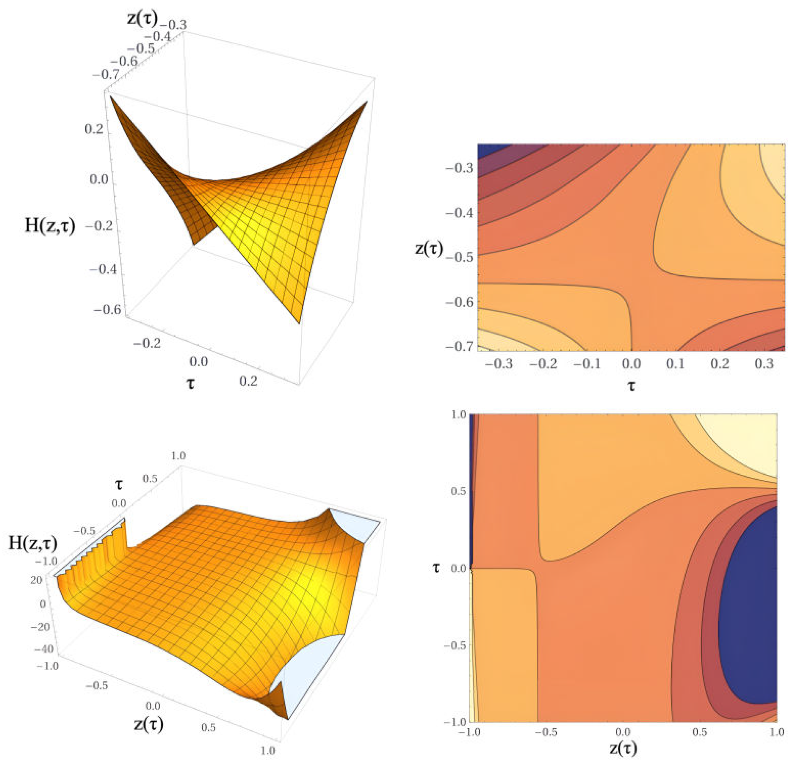
Figure 10 shows on the left 3D graphs of the potential defined in Equation (36) and on the right the corresponding 2D contour plots for and a combination of parameters that obey the naturalness condition for long-range and fine-tuning for short-range values of , with . The results for the additional values of fine-tuning parameters lead to very similar figures.
The image in figure (Figure 10) reveal that the mutative symplectic algebraic structure can generate, through a certain combination of parameters, a peculiar type of space-time deformation that materializes, among other aspects, in the overcoming of the alignment of the infinitely countable number of poles arranged in a straight line, identified by the white band in the color palette of the contour plots, replacing it by a smooth transition in the form of a space-time twist, with its shear center located at the temporal transition point between the mirror universe and its current counterpart. This result, like the previous cases, offers an alternative to the quantum topological jump, manifested in a smooth transition between the mirror universe and its current counterpart as well as a kind of `space-time deformation memory attractor’, allowing the universe to recover its `initial’ shape in the conformation region around the transition of the shear center of the twist in good agreement with the proposal of Vasak et al. [27]. The boundary conditions, in turn, similarly to the previous cases, are in tune with the Bekenstein criterion, allowing the transition of quantum solutions from the scale factor through a quantum topological jump.
5.1. Solutions - recursive approach
We adopt a recursive approach to find a consistent solution to equation (34), despite its formal complexity. Assuming a nonempty recursion loop, we solve equation (34) by integrating both sides of the equation, treating the scale factor with an implicit time dependence on the left-hand side of this equation, while the right-hand side has an explicit time dependence on and . This assumption allows to find a solution by means of a recursion procedure which refers to a function calling itself directly or even indirectly. Of course, we may invoke a kind of test or verification that the condition `empty loop’ is fulfilled as a condition that the function should (may) call itself. The family of sample solutions of equation (34) shown in Figure 11 reveals the impact of the non-commutative symplectic structure on the behavior of the BCQG scale factor. Among the distinct curves that describe the evolution of as a function of , those that reveal an accelerated growth of the scale factor stand out. These results are in line with the BCQG proposal of identifying the non-commutative symplectic structure as the driver of the acceleration of the universe.
5.2. BCQG Hubble parameter (Hubble rate)
Combining equations (34) and (35), the BCQG Hubble parameter (Hubble rate) becomes
Figure (Figure 12) shows the behavior of the Hubble parameter for a particular fine-tuning set of parameters. The standard way of determining the Hubble constant involves gauging precise distances to galaxies using standard candles, for which the apparent brightness can be compared to the `true’ luminosity. In contrast, by analyzing temperature fluctuations in the cosmic microwave background (CMB), cosmological models allow the current rate of expansion of the universe to be determined. Among the enigmas of current cosmology, the so-called `Hubble tension’ attracts attention: the current expansion rate of the universe is faster than expected, either based on the cosmological initial conditions or on our current understanding of the evolution of the universe. At the moment we seek to understand the outcome for the Hubbler rate given in equation (37), since these questions may guide our future prospects for BCQG. The BCQG proposal, in its current stage of formal development, can contribute little to dispel the Hubble tension. This is because the BCQG describes an evolutionary cosmos at a stage much earlier than the recombination era, the period of emission of the first light in the universe. When we examine the results presented in figure (Figure 12), the behavior of the Hubble rate presents very unique characteristics. And since we are using a parameterization based on a fine-tuning perspective, in order to make contact with current observations and current theoretical proposals, instead of adopting the naturalness conception, these unique characteristics are certainly affected and even shaped by the choices of the running coupling constants. Nevertheless, we can identify in the images in the figure (Figure 12) intricate aspects in the behavior of , which demonstrate, in view of the previous results, the intrinsic nature of the foliated quantum formulation, therefore going beyond the simple choice of the formulation parameters. The Hubble constant, technically, corresponds to the reciprocal of time. Thus, during the period in which Planck time predominates, the value of the Hubble constant is extremely high. Our calculations for are in line with these expectations, as can be seen in Figure 12. The results also show great formal consistency insofar as the time dependence in the scale factor, despite a dimensionless quantity, corresponds to an implicit time dependence, not an explicit dependence. Thus, insofar as the scale factor corresponds to a dimensionless variable, in turn has an inverse dependence on time comprising in the region of study values of the order of Fermi inverse time scale. The results reveal a wide spectrum of values of , ranging from , in the region that encompasses the transition phase between the mirror universe and the current one, to , to , for time values corresponding to the interval to . Using the scale transformation parameter km/ Mpc , taking the previous time-range, the spectrum of values for the Hubble parameter scans large values ranging from km to km .
5.3. BCQG redshift cosmological parameter
In simple terms, the expansion of the universe stretches the wavelength of electromagnetic radiation traveling through space, generating the phenomenon known as `cosmological redshift’, so that for larger values of the redshift, the greater the distances that the light has traveled.
Assuming for simplicity , where corresponds to the present time age of the universe, the following BCQG scale factor and the cosmological redshift parameter relation then holds
and a recursive approach, from equation (34) combined with (35), the following equation results
with defined as
Figure 13 shows the behavior of the solution of equation (39). Taking a step back in the definition of the BCQG cosmological redshift, may be expressed as
where and represents the present time and primordial time universe radius.
The results indicate two surprising aspects. The first aspect refers to an extremely large universe radius in the transition region between the two universes, rapidly expanding to higher values. The second aspect indicates a persisting tension between blueshift and redshift, implying a decrease in wavelength and an increase in frequency and energy, or a negative redshift.
Assuming a shell model for the primordial mirror universe, a background light source due to the uncountable physical processes related to the violent contraction phase will produce a redshift shadow of the contraction phase. Then the opposite process would occur in the expansion phase. However, what we see in the left image Figure 13 is a combination in the contraction and expansion phases of positive and negative values of , which characterize a combination of the red-shift and blue-shift processes, despite the overpowering predominance of the former. The image on the right of Figure 13, showing the slope field curves, indicates that the negative values exhibit residual behavior while the negative values decrease from the contraction phase to the contraction phase, while the behavior in the expansion phase is reversed. Therefore, the contraction phase is characterized by the rapid decrease of the BCQG redshift cosmological parameter, while the expansion phase is characterized by the rapid growth of .
5.4. Redshift dependence of the BCQG Hubble parameter
Combining equations (37) and (38) the following relation holds for the BCQG Hubble parameter as a function of the BCQG redshift cosmological parameter:
The top left image above of Figure 14 reveals, during a small window of primordial time, the behavior of , near the transition between the two phases of the universe, where the blue shift behavior stands out. The top right image above shows the corresponding contour plot. The images below Figure 14 correspond to the behavior of in a litle more extended time window. The upper left image also reveals, once again, although devoid of a theoretical basis so far, a behavior typical of the presence of a torsion. This topic, taking into account the Einstein–Hilbert action as a paradigmatic starting point, must assume the presence of an asymmetric affine connection rather than the symmetric connection of the Levi–Civita type, where spacetime is subjected to a torsion in addition to curvature, and then the metric and the torsion are varied independently.
6. Final Remarks and Conclusion
The BCQG framework stands out as a significant generalization of the standard Friedmann equations, as it addresses the gaps in conventional inflationary models and introduces a richer mathematical structure to study the evolution of the universe. The UV/IR interplay, a defining feature of noncommutative systems, proves to be a compelling mechanism for elucidating inflationary dynamics while overcoming key shortcomings of classical models. Moreover, the incorporation of quantum gravity effects into the cosmological equations lends theoretical robustness to the proposed framework.
The results of the wave function present unique and consistent characteristics and similarities. The evolutionary behavior for both solutions indicates a cyclical and rapidly expanding Universe, with the amplitudes of both wave functions, and , systematically increasing in contrast to the systematic reduction of the corresponding Planck time intervals, a compelling indication of cosmic acceleration in the inflationary period.
To our knowledge, this is the first time that solutions of a wave equation of an inflaton field are known, in the context of quantum gravity, evidencing related and complementary behavior of the inflaton field and the cosmic scale factor. These results further indicate that the conventional inflation model, although historically introduced in an ad hoc manner, includes crucial elements that characterize the cosmic acceleration drive.
This behavior indicates a growing disruptive evolution increase in the branched-gravitation expansion phase, prior to the BCQG transition region characterized by the overcoming of the primordial singularity, as predicted in the standard model, and prior to the wave-contraction phase.
Furthermore, when we consider the dynamical equations involving the cosmic scale factor, the presence of the inflaton field in the present formulation of BCQG adheres consistently to the reconfiguration of spacetime as a result of a non-commutative symplectic algebraic structure, contributing in a unique manner for cosmic acceleration.
The branched transition region can be outlined according to three different perspectives: (i) a classical view of a kind of ‘transition topological portal’, (ii) a quantum view region that contemplates a topological quantum leap, and (iii) a mixed conception in which both previous conceptions intersect consistently, shaped according to the Bekenstein criterion (see [1]). The topologically foliated branch cut quantum structural representation of the transition region involving the contraction and expansion phases resembles a topological spacetime shortcut, as a kind of foliated wormhole structure. Theoretical implications of the existence of topological shortcuts in spacetime imply a challenge to our understanding of fundamental physical principles such as causality or still open topics such as the origin of primordial cosmological material seeds. Accordingly, the standard inflation model conception of the creation of the present Universe from nothing, as a result of virtual vacuum fluctuations, falls apart. Our results indicate that the present Universe might have its origin in an earlier phase through a possible distant space-time shortcut. We may conjecture if this tiny correction would be, in principle, detectable by homodyne-type measurements, — a method of extracting information encoded as modulation of the phase and/or frequency of an oscillating signal, a gravitational wave for instance. Additionally, we may even conjecture that this tiny correction would be detectable after long propagation lengths for a wide range of throat radii and distances to the shortcut, even if the detection takes place very far away from the throat, where the spacetime is very close to a flat geometry.
In conclusion, our study establishes the BCQG framework as a promising alternative to standard inflationary models, providing new insights into the dynamics of the early universe. The modified Friedmann equations derived in this context illuminate the role of non-commutative geometry in driving cosmic inflation and predict observable phenomena such as relic gravitational waves, which could serve as experimental probes for validating the theory.
Future research could focus on aligning these predictions with current astrophysical observations, exploring numerical simulations to validate the predictions of the framework, and expanding the theoretical model to include additional interactions or higher-order corrections. Our work lays a solid foundation for the integration of foliated non-commutative quantum gravity into cosmology and presents innovative avenues for understanding the origins and evolution of the universe.
Author Contributions
Conceptualization, C.A.Z.V.; methodology, C.A.Z.V. and B.A.L.B. and P.O.H and J.A.deF.P. and D.H. and F.W. and M.M. and R.R.; software, C.A.Z.V. and B.A.L.B. and M.R. and M.M.; validation, C.A.Z.V. and B.A.L.B. and D.H. and P.O.H. and J.A.deF.P. and F.W. and R.R.; formal analysis, C.A.Z.V. and B.A.L.B. and P.O.H. and J.A.deF.P. and D.H. and F.W. and R.R.; investigation, C.A.Z.V. and B.A.L.B. and P.O.H. and J.A.deF.P. and M.R. and M.M. and F.W. and R.R.; resources, C.A.Z.V.; data curation, C.A.Z.V. and B.A.L.B.; writing—original draft preparation, C.A.Z.V.; writing—review and editing, C.A.Z.V. and B.A.L.B. and P.O.H. and J.A.deF.P. and D.H. and M.R. and M.M. and F.W.; visualization, C.A.Z.V. and B.A.L.B.; supervision, C.A.Z.V.; project administration, C.A.Z.V.; funding acquisition (no funding acquisition). All authors have read and agreed to the published version of the manuscript..
Acknowledgments
P.O.H. acknowledges financial support from PAPIIT-DGAPA (IN116824). F.W. is supported by the U.S. National Science Foundation under Grant PHY-2012152.
References
- Zen Vasconcellos, C.A.; Hess, P.O.; de Freitas Pacheco, J.; Weber, F.; Bodmann, B.; Hadjimichef, D.; Naysinger, G.; Netz-Marzola, M.; Razeira, M. The Accelerating Universe in a Noncommutative Analytically Continued Foliated Quantum Gravity. Classical and Quantum Gravity 2024.
- Zen Vasconcellos, C.A.; Hess, P.O.; de Freitas Pacheco, J.; Weber, F.; Bodmann, B.; Hadjimichef, D.; Naysinger, G.; Netz-Marzola, M.; Razeira, M. Cosmic inflation in an extended non-commutative foliated quantum gravity: the wave function of the universe. Submitted to Universe 2025.
- Friedman, A. Über die Krümmung des Raumes. Zeitschrift für Physik 1922, 10, 377–386. [Google Scholar] [CrossRef]
- Lemaître, G. Un Univers homogène de masse constante et de rayon croissant rendant compte de la vitesse radiale des nébuleuses extra-galactiques. Annales de la Société Scientifique de Bruxelles 1927, A47, 49. [Google Scholar]
- Robertson, H.P. Kinematics and World-Structure. Astrophysical Journal 1935, 82, 248–301. [Google Scholar] [CrossRef]
- Walker, A.G. On Milne’s Theory of World-Structure. Proceedings of the London Mathematical Society 1937, 42, 90. [Google Scholar] [CrossRef]
- Arnowitt, R.; Deser, S.; Misner, C.W. The dynamics of general relativity (republication). General Relativity and Gravitation 2008, 40, 1997–2027. [Google Scholar] [CrossRef]
- Zen Vasconcellos, C.A.; Hadjimichef, D.; Razeira, M.; Volkmer, G.; Bodmann, B. Pushing the Limits of General Relativity Beyond the Big Bang Singularity. Astron. Nachr. 2019, 340, 857–865. [Google Scholar] [CrossRef]
- Zen Vasconcellos, C.A.; Hess, P.O.; Hadjimichef, D.; Bodmann, B.; Razeira, M.; Volkmer, G.L. Pushing the Limits of Time Beyond the Big Bang Singularity: The branch cut universe. Astron. Nachr. 2021, 342(5), 765–775. [Google Scholar] [CrossRef]
- Zen Vasconcellos, C.A.; Hess, P.O.; Hadjimichef, D.; Bodmann, B.; Razeira, M.; Volkmer, G.L. Pushing the Limits of Time Beyond the Big Bang Singularity: Scenarios for the branch-cut Universe. Astron. Nachr. 2021, 342(5), 776–787. [Google Scholar] [CrossRef]
- Bodmann, B.; Zen Vasconcellos, C.A.; Hess, P.O.; de Freitas Pacheco, J.A.; Hadjimichef, D.; Razeira, M.; Degrazia, G.A. A Wheeler–DeWitt Quantum Approach to the Branch-Cut Gravitation with Ordering Parameters. Universe 2023, 9(6), 278. [Google Scholar] [CrossRef]
- Bodmann, B.; Hadjimichef, D.; Hess, P.O.; de Freitas Pacheco, J.; Weber, F.; Razeira, M.; Degrazia, G.A.; Marzola, M.; Zen Vasconcellos, C.A. A Wheeler-DeWitt Non-commutative Quantum Approach to the Branch-cut Gravity. Universe 2023, 9(10), 428. [Google Scholar] [CrossRef]
- Weyl, H. Reine Infinitesimalgeometrie. Math. Zeit. 1918, 2, 384. [Google Scholar] [CrossRef]
- Weyl, H. Über die Definitionen der mathematischen Grundbegriffe. Mathematisch-naturwissenschaftliche Blatter 1910, 7, 93–95. [Google Scholar]
- Guth, A.H. Inflationary universe: A possible solution to the horizon and flatness problems. Phys. Rev. 1981, D23, 347–356. [Google Scholar] [CrossRef]
- Guth, A.H. Carnegie Observatories Astrophysics Series, Vol. 2: Measuring and Modeling the Universe; W. L. Freedman (ed.); Cambridge Univ. Press: London, UK, 2004. [Google Scholar]
- Bertolami, O.; Zarro, C.A.D. Hořava-Lifshitz quantum cosmology. Phys. Rev. D 2011, 84, 044042. [Google Scholar] [CrossRef]
- Maeda, K.I.; Misonoh, Y.; Kobayashi, T. Oscillating Bianchi IX Universe in Hořava-Lifshitz Gravity. Phys. Rev. D 2010, 82, 064024. [Google Scholar] [CrossRef]
- de Alfaro, V.; Fubini, S.; Furlan, G. Conformal invariance in quantum mechanics. Nuovo Cimento A 1976, 34, 569. [Google Scholar] [CrossRef]
- Feinberg, J.; Peleg, Y. Self-adjoint Wheeler-DeWitt operators, the problem of time, and the wave function of the Universe. Phys.Rev. D 1995, 52, 1988. [Google Scholar] [CrossRef]
- Friedman, A. Über die Möglichkeit einer Welt mit konstanter negativer Krümmung des Raumes. Zeitschrift für Physik 1924, 21, 326–332. [Google Scholar] [CrossRef]
- Hawking, S.W.; Hertog, T.J. A smooth exit from eternal inflation? High Energ. Phys. 2018, 04, 147. [Google Scholar] [CrossRef]
- Adler, R.; Bazin, M.; Schiffer, M. Introduction to General Relativity; McGraw-Hill: New York, USA, 1965. [Google Scholar]
- Ellis, G.F.R. The arrow of time and the nature of spacetime. Studies in History and Philosophy of Science Part B: Studies in History and Philosophy of Modern Physics 2013, 44 (3), 242–262.
- Ellis, G.F.R. Time really exists! The evolving block universe. euresis journal 2014, 7, 1–16. [Google Scholar]
- Rovelli, C. The strange equation of quantum gravity. Class. Quantum Grav. 2015, 32, 124005. [Google Scholar] [CrossRef]
- van de Venn, A.; Vasak, D.; Kirsch, J.; Struckmeier, J. Torsional dark energy in quadratic gauge gravity. Eur. Phys. J. C 2023, 83, 288. [Google Scholar] [CrossRef]
Figure 1.
On the left, 3D plot for the real parts of the potential defined in equation (32), for chaotic inflation simulation. On the right, the corresponding contour plot. Assuming a fine-tuning set of the cosmological initial, the corresponding parameters are: ; ; ; ; ; ; ; .
Figure 1.
On the left, 3D plot for the real parts of the potential defined in equation (32), for chaotic inflation simulation. On the right, the corresponding contour plot. Assuming a fine-tuning set of the cosmological initial, the corresponding parameters are: ; ; ; ; ; ; ; .
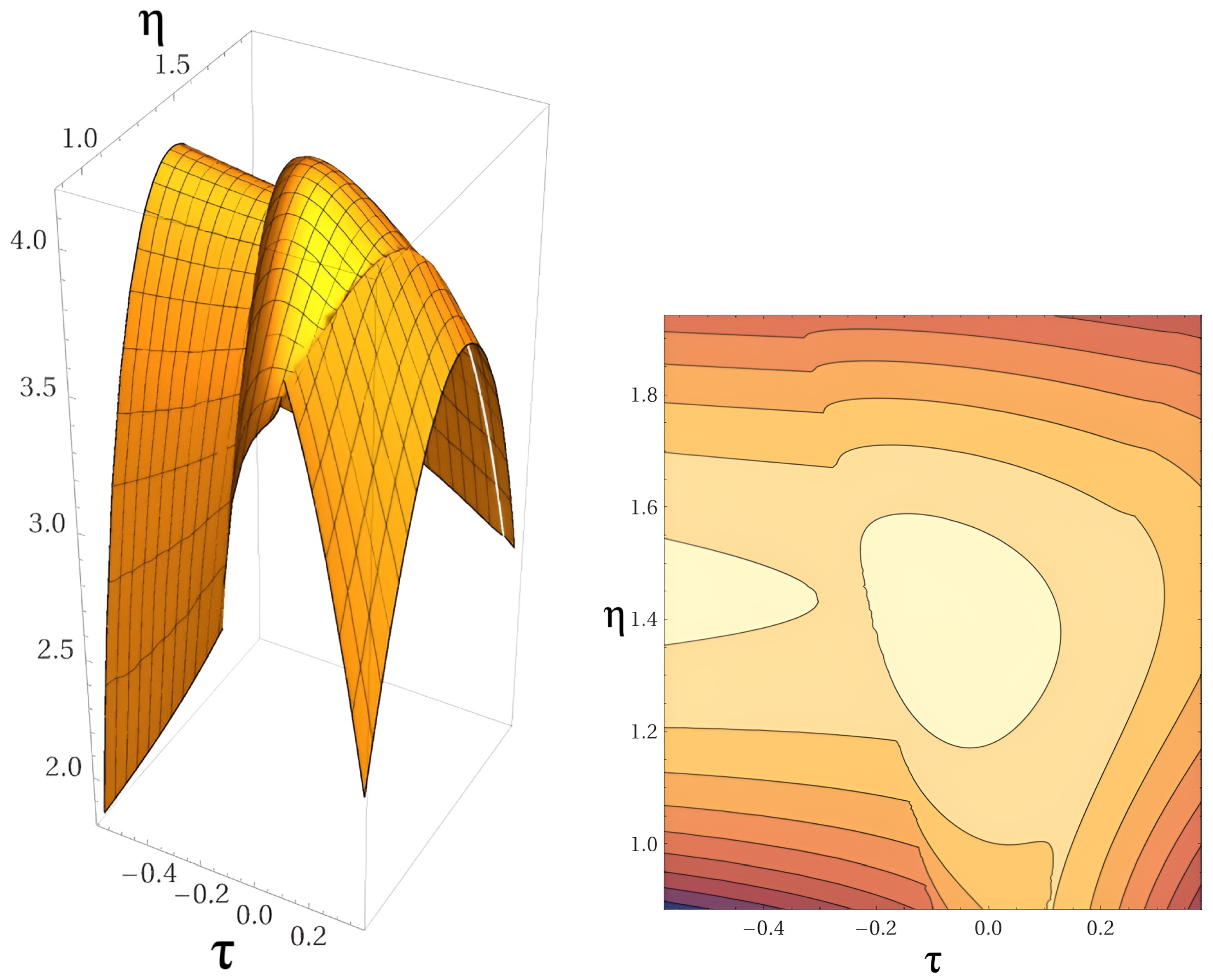
Figure 2.
On the left, 3D plot for the imaginary part of the potential defined in equation (32), for chaotic inflation simulation. On the right, the corresponding contour plot. Assuming a fine-tuning set of the cosmological initial, the corresponding parameters are: ; ; ; ; ; ; ; .
Figure 2.
On the left, 3D plot for the imaginary part of the potential defined in equation (32), for chaotic inflation simulation. On the right, the corresponding contour plot. Assuming a fine-tuning set of the cosmological initial, the corresponding parameters are: ; ; ; ; ; ; ; .
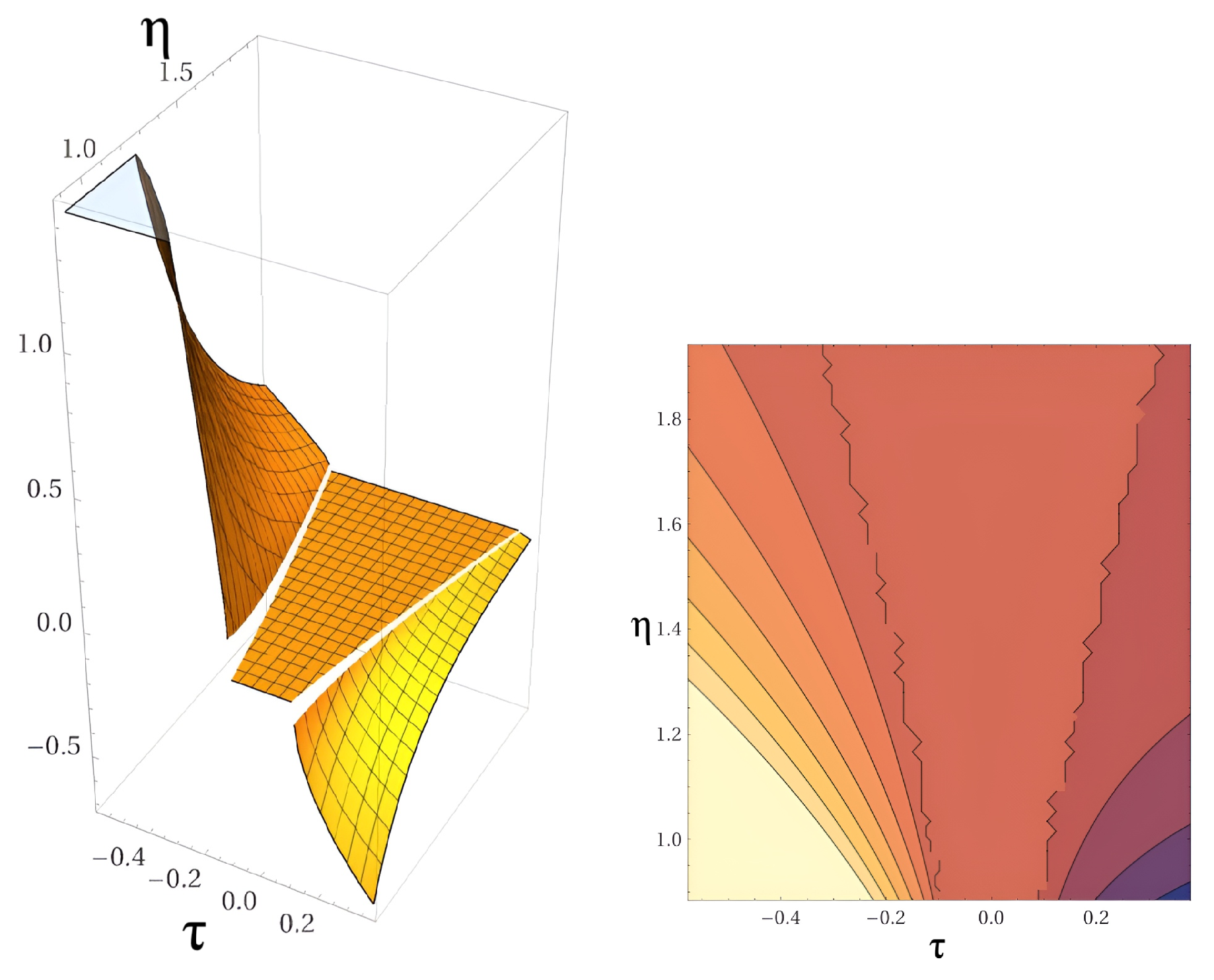
Figure 3.
On the left, 3D plot for the real part of the potential defined in equation (33), for non-chaotic inflation simulation. On the right, the corresponding contour plot. The parameters are: ; ; ; ; ; ; ; .
Figure 3.
On the left, 3D plot for the real part of the potential defined in equation (33), for non-chaotic inflation simulation. On the right, the corresponding contour plot. The parameters are: ; ; ; ; ; ; ; .
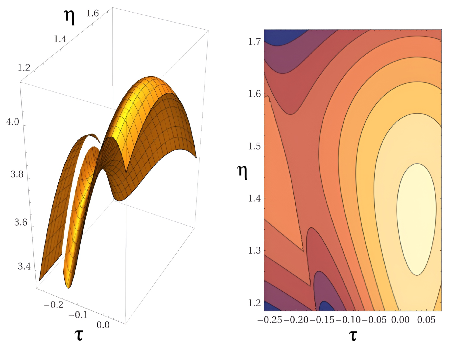
Figure 4.
On the left, 3D plots for the imaginary part of the potential defined in equation (33), for non-chaotic inflation simulation. On the right, the corresponding contour plot. The parameters are: ; ; ; ; ; ; ; .
Figure 4.
On the left, 3D plots for the imaginary part of the potential defined in equation (33), for non-chaotic inflation simulation. On the right, the corresponding contour plot. The parameters are: ; ; ; ; ; ; ; .
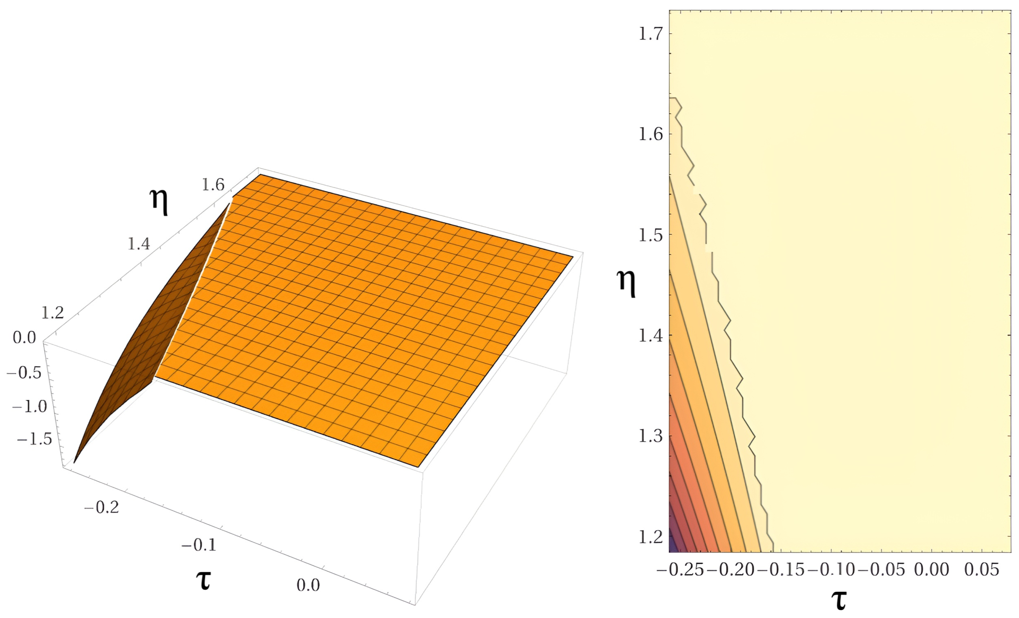
Figure 5.
Sample solutions of equation (31) for , assuming the naturalness condition, with the potential (32) restricted to the contribution of the field. On the left, corresponding to sample family solutions, the figure shows a cross-section structure corresponding to the distribution of real and imaginary numerical sample solutions of the wave-function . On the right, the figure shows plots of sample individual solutions, with , where the blue lines correspond to the real part while orange lines to imaginary solutions.
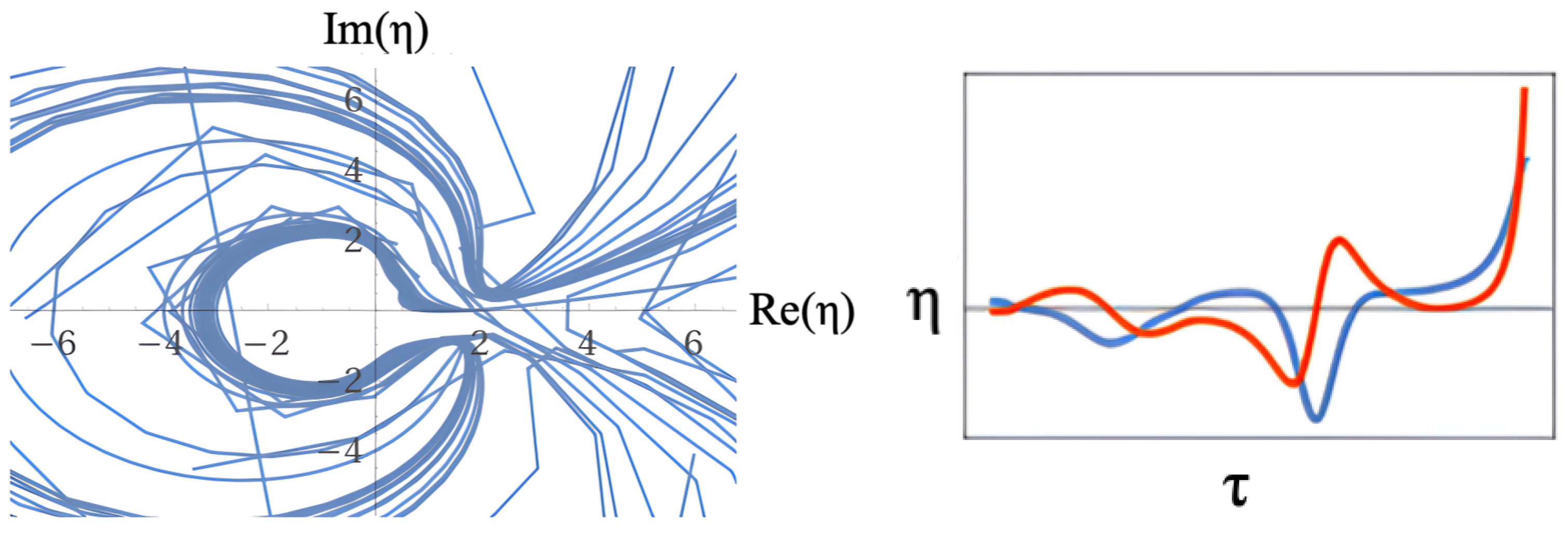
Figure 6.
Sample solutions of equation (31) for , assuming the naturalness condition, with the complete structure of the potential (32), more specifically with the contribution of the and fields and with the term modeling chaotic inflation. On the left, sample solution family. The figure shows an Argand-type structure corresponding to the distribution of real and imaginary numerical sample solutions of the wave-function . On the right, plots of sample individual solutions, with , where the blue lines correspond to the real part while orange lines to imaginary solutions.
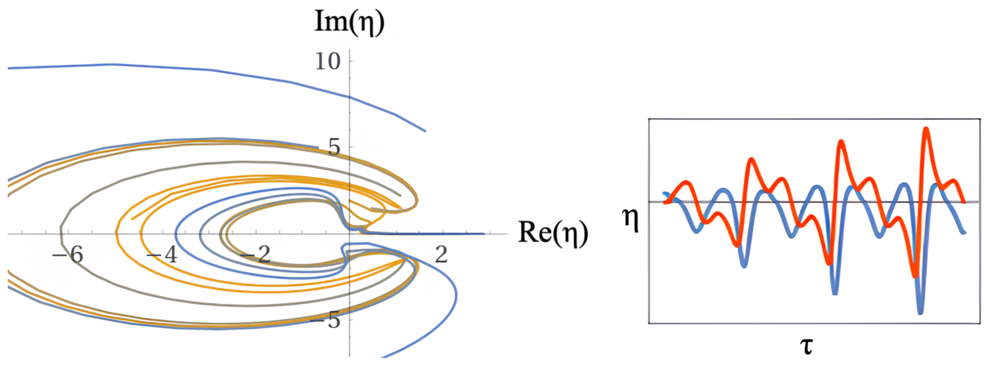
Figure 7.
Sample solutions of equation (31) for , assuming the naturalness condition, with the complete structure of the potential (32), more specifically with the contribution of the and fields and with the term modeling non-chaotic inflation. On the left, sample solution family. The figure shows an Argand-type structure corresponding to the distribution of real and imaginary numerical sample solutions of the wave-function . On the right, plots of sample individual solutions, with , where the blue lines correspond to the real part while orange lines to imaginary solutions.
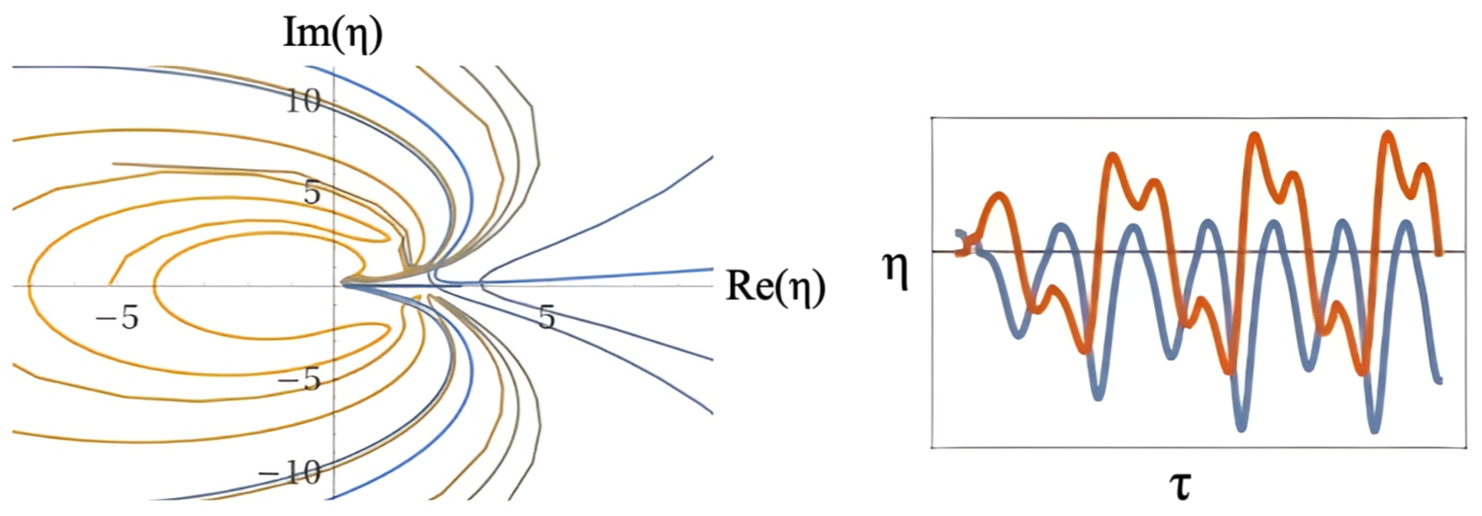
Figure 8.
On the left, 3D plot of the potential defined in equation (35). On the right the corresponding 2D contour plot. On the figures, a combination of parameters obeying the naturalness condition for long-range and fine-tuning for short-range values of , with , was assumed, together with and .
Figure 8.
On the left, 3D plot of the potential defined in equation (35). On the right the corresponding 2D contour plot. On the figures, a combination of parameters obeying the naturalness condition for long-range and fine-tuning for short-range values of , with , was assumed, together with and .
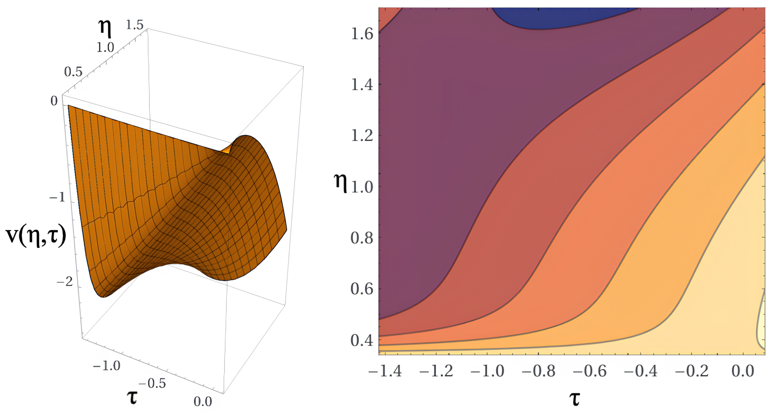
Figure 9.
On the left, 3D plot of the potential defined in equation (35). On the right the corresponding 2D contour plot. On the figures it was assumed the following fine-tunning set of parameters: ; ; ; ; ; ; .
Figure 9.
On the left, 3D plot of the potential defined in equation (35). On the right the corresponding 2D contour plot. On the figures it was assumed the following fine-tunning set of parameters: ; ; ; ; ; ; .
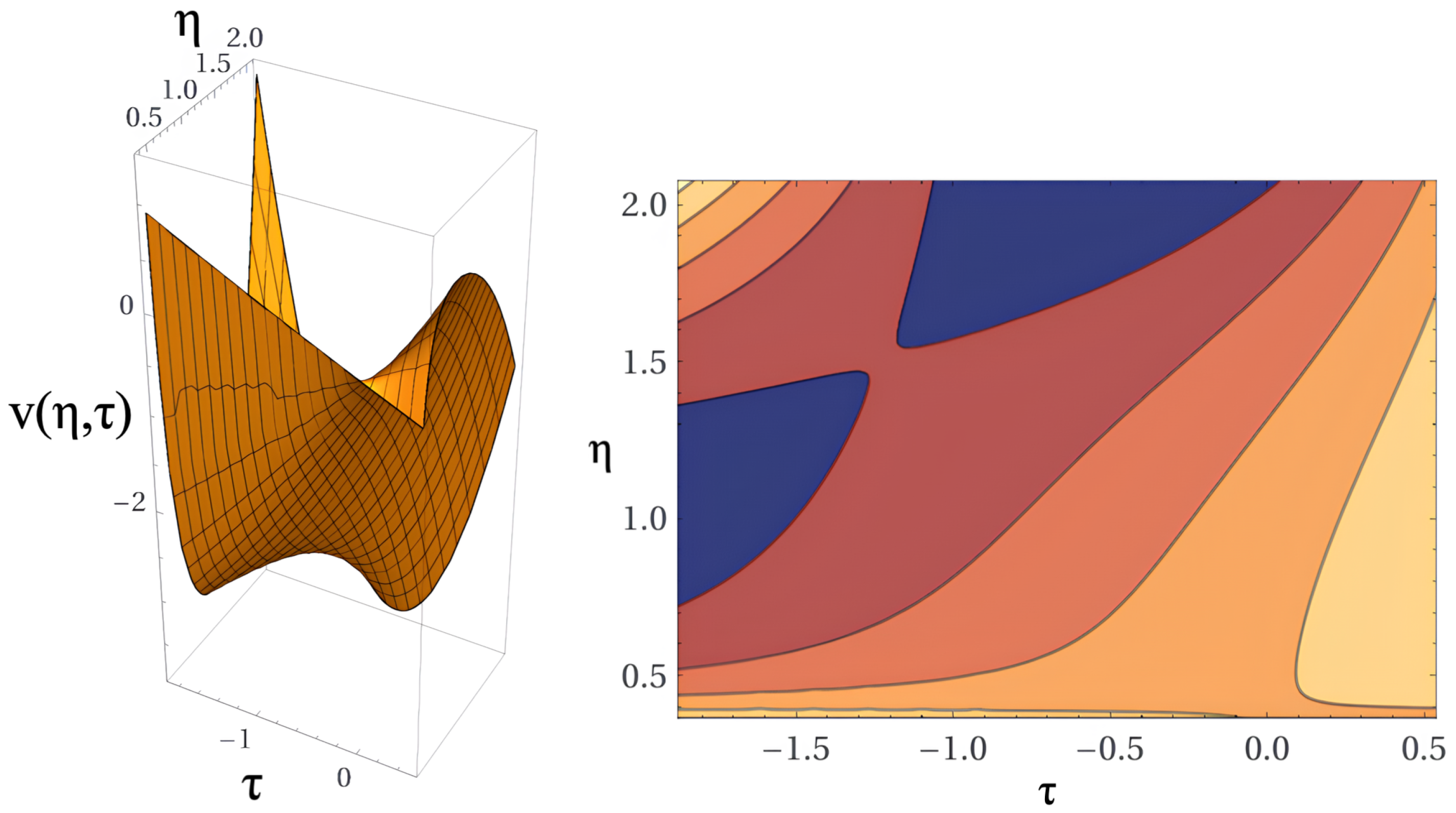
Figure 10.
On the left, 3D plot of the potential defined in equation (36). On the right the corresponding 2D contour plot. On the figures, a combination of parameters obeying the naturalness condition for long-range and fine-tuning for short-range values of , with , was assumed, together with .
Figure 10.
On the left, 3D plot of the potential defined in equation (36). On the right the corresponding 2D contour plot. On the figures, a combination of parameters obeying the naturalness condition for long-range and fine-tuning for short-range values of , with , was assumed, together with .
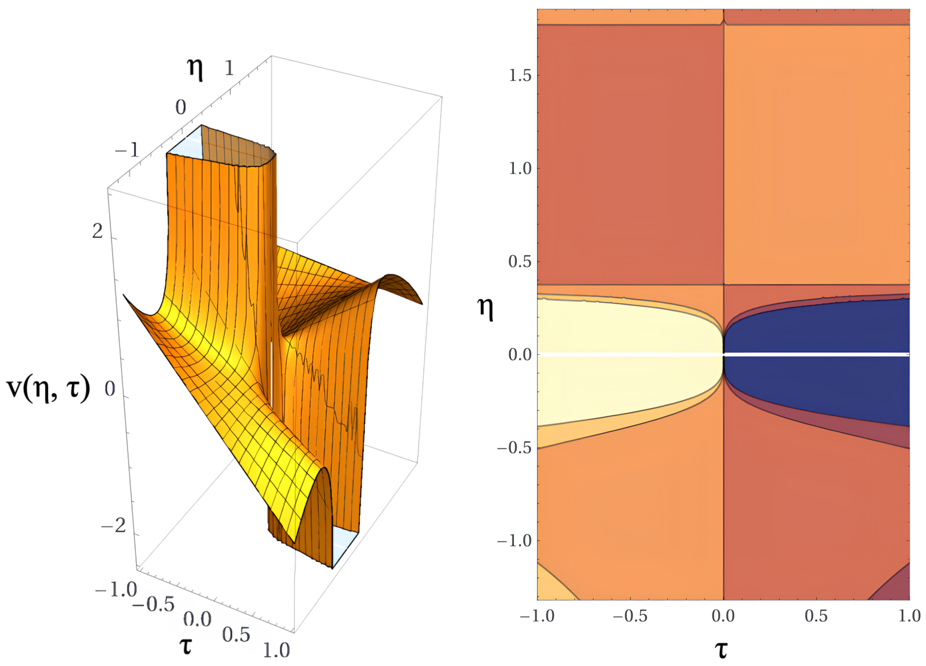
Figure 11.
On the figures, plots of sampling solutions of equation (34 with the potential given in equation (vetat+) for the initial condition . On the left image, the combination of parameters obeying the naturalness condition for long-range and fine-tuning for short-range values of , with , was assumed, together with and . On the right image it was assumed the following fine-tunning set of parameters: ; ; ; ; ; ; .
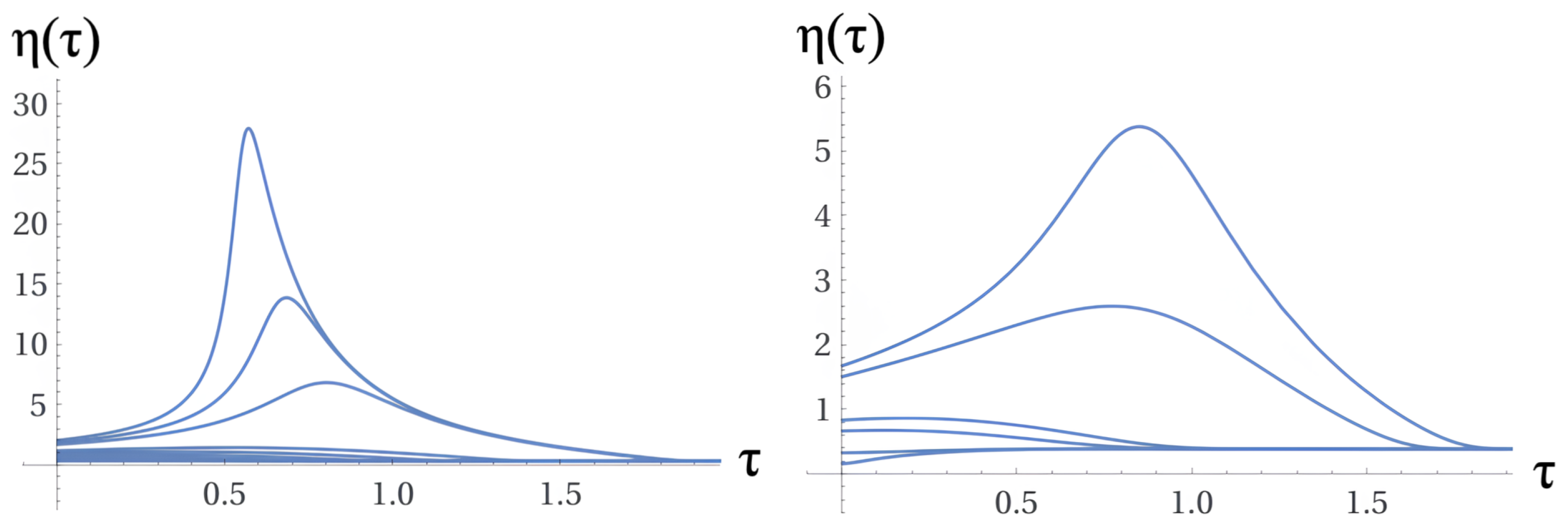
Figure 12.
The figures display the behavior of the Hubble parameter for a particular fine-tuning set of parameters to make contact with observations and more conventional models: ; ; ; ; ; ; ; . On the left figure, the image shows a 3D plot of the real part of while on the right the 2D corresponding contour plot.
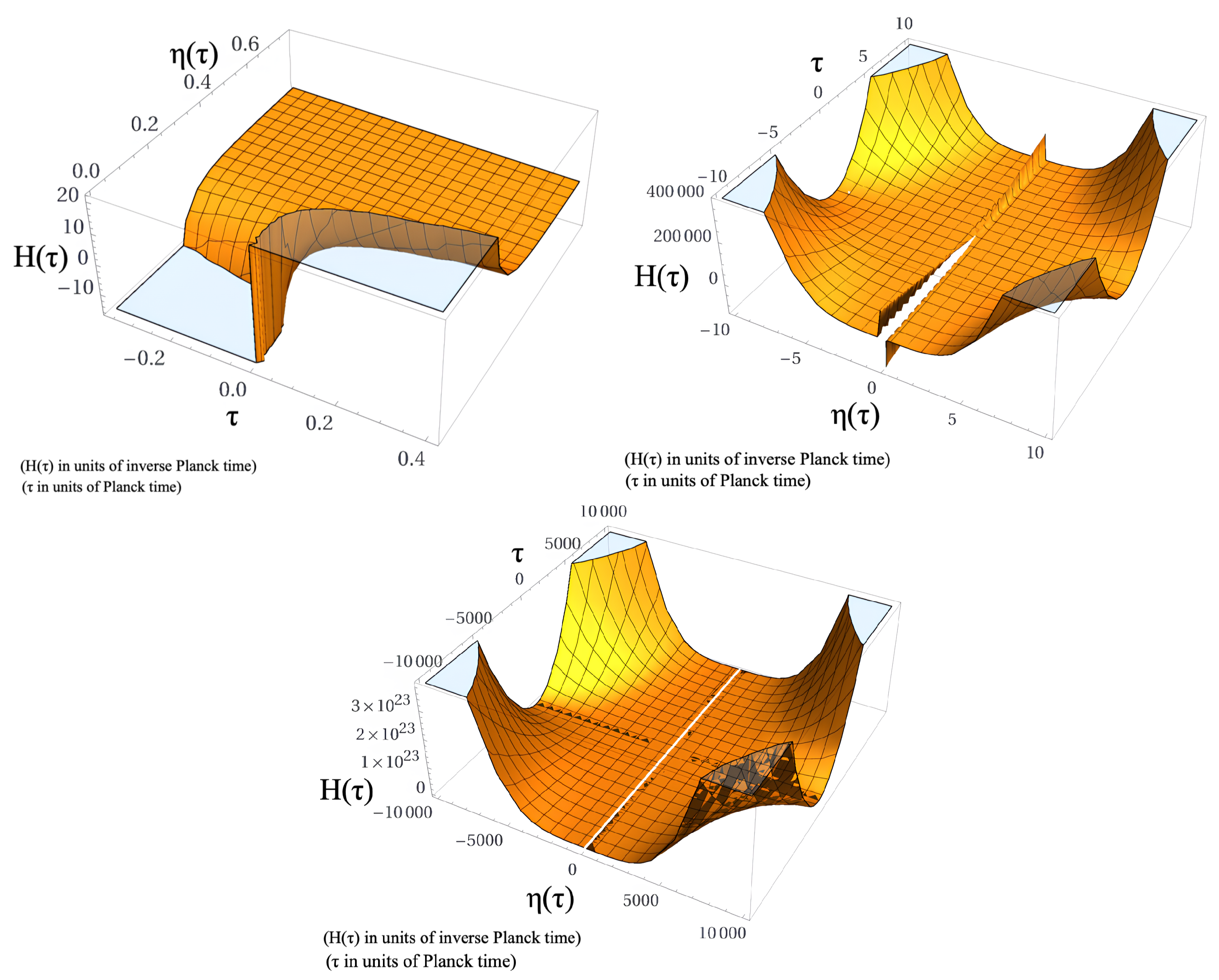
Figure 13.
The figure on the left display the behavior of the BCQG redshift cosmological parameter for a particular fine-tuning set of parameters to make contact with observations and more conventional models: ; ; ; ; ; ; ; . The figure on the right shows the corresponding behavior of the field slope of .
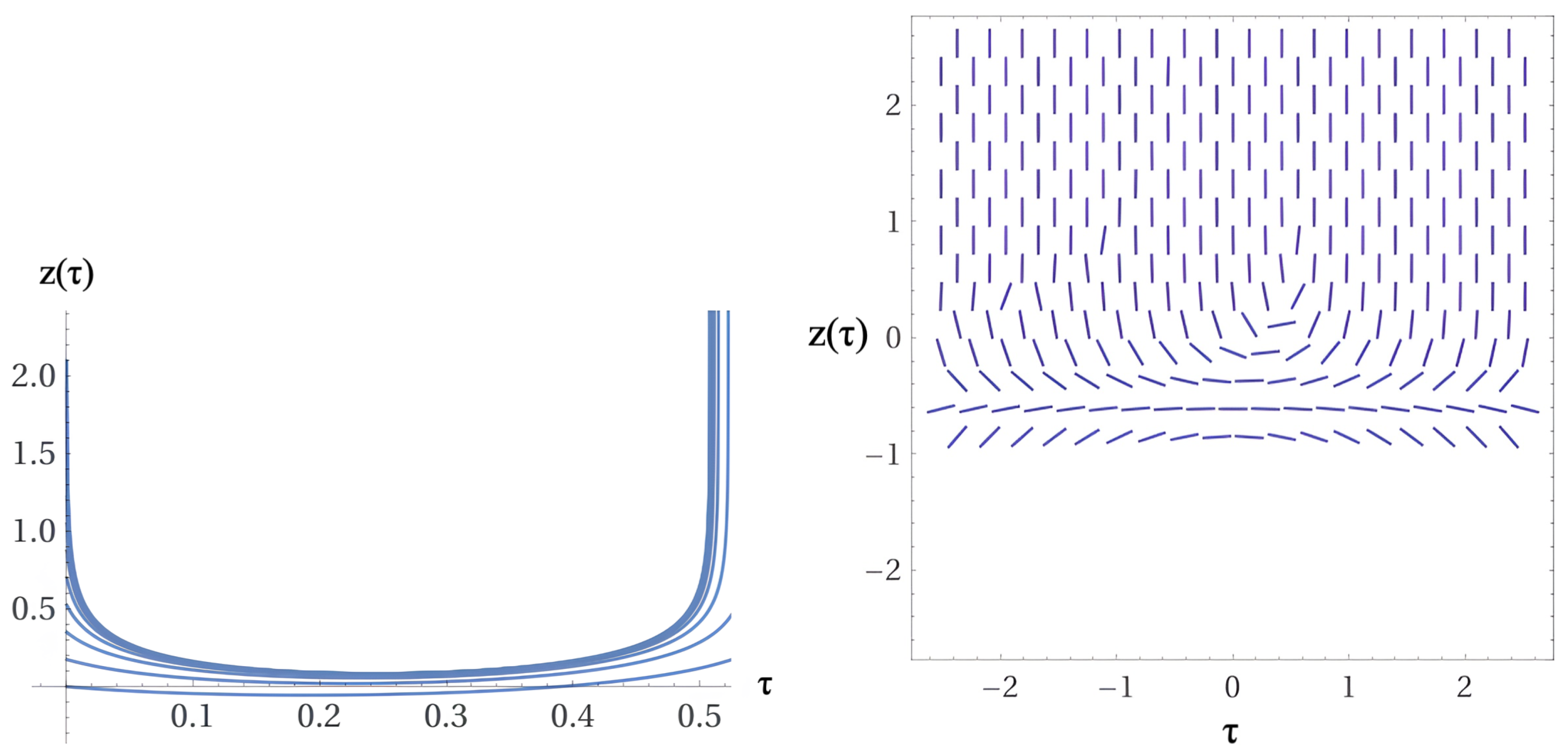
Figure 14.
The figures display, for different time ranges, on the left, the behavior of the BCQG parameter and, on the right, the corresponding contour plot of vs , for a particular fine-tuning set of parameters to make contact with observations and more conventional models: ; ; ; ; ; ; ; .
Figure 14.
The figures display, for different time ranges, on the left, the behavior of the BCQG parameter and, on the right, the corresponding contour plot of vs , for a particular fine-tuning set of parameters to make contact with observations and more conventional models: ; ; ; ; ; ; ; .
Disclaimer/Publisher’s Note: The statements, opinions and data contained in all publications are solely those of the individual author(s) and contributor(s) and not of MDPI and/or the editor(s). MDPI and/or the editor(s) disclaim responsibility for any injury to people or property resulting from any ideas, methods, instructions or products referred to in the content. |
© 2025 by the authors. Licensee MDPI, Basel, Switzerland. This article is an open access article distributed under the terms and conditions of the Creative Commons Attribution (CC BY) license (http://creativecommons.org/licenses/by/4.0/).
Copyright: This open access article is published under a Creative Commons CC BY 4.0 license, which permit the free download, distribution, and reuse, provided that the author and preprint are cited in any reuse.


