
Submitted:
08 April 2025
Posted:
14 April 2025
You are already at the latest version
Abstract
Remote sensing image change detection, being a pixel-level dense prediction task, requires both high speed and high accuracy. The redundancy within the models and detection errors, particularly missed detection, generally affect accuracy and merit further research. Moreover, the former also leads to a reduction in speed. To guarantee the efficiency of change detection, encompassing both speed and accuracy, a VMamba-based Multi-scale Feature Guiding Fusion Network (VMMCD) is proposed. This network is capable of promptly modeling global relationships and realizing multi-scale feature interaction. Specifically, Mamba backbone is adopted to replace the commonly used CNN and Transformer backbones. By leveraging VMamba’s global modeling ability with linear computational complexity, the computational resources needed for extracting global features are reduced. Secondly, considering the characteristics of the VMamba model, a compact and efficient lightweight network architecture was devised. The aim is to reduce the model’s redundancy, thereby avoiding the extraction or introduction of interfering and redundant information. As a result, the speed and accuracy of the model are both enhanced. Finally, the Multi-scale Feature Guiding Fusion (MFGF) module is developed, which strengthen the global modeling ability of VMamba. Additionally, it enriches the interaction among multi-scale features to address the common issue of missed detection in changed areas. The proposed network has achieved competitive results on three datasets, and remarkably surpasses the current state-of-the-art performance on SYSU-CD, with F1 of 83.35% and IoU of 71.45%. Moreover, for inputs of 256×256 size, it is more than three times faster than the current state-of-the-art Mamba-based change detection model. This outstanding achievement demonstrates the effectiveness of our proposed approach.
Keywords:
change detection
; VMamba
; state space model
; multi-scale feature guiding fusion
; high resolution remote sensing image
1. Introduction
With the increasing importance of remote sensing technology, the domain of change detection has progressively gained prominence. Change detection aims to identify changes between scenes at different time phases. Through the identification of such changes, efficacious scene monitoring can be achieved. Consequently, change detection finds extensive application in a diverse array of fields, encompassing forest vegetation monitoring [1], urban planning [2,3,4], land cover change analysis [5], disaster monitoring and evaluation [6], and military reconnaissance[7].
Conventional methodologies employed in change detection tasks generally encompass two sequential steps: unit analysis and change identification [8]. In light of the selected unit, pixel-based approaches [9] and object-based approaches [10] are available. Nevertheless, the progress in optical Very High Resolution (VHR) imaging has led to a continuous enhancement in image resolution, thereby presenting more detailed characteristics, including the texture and geometric structure of ground objects. This enhancement has, in turn, given rise to an increasing heterogeneity within regions of the same spatial scale, significantly constraining the robustness and effectiveness of traditional change detection approaches.
With the continuous evolution of software and hardware configurations, deep learning-based change detection methods have progressively gained wider acceptance. These methods have significantly enhanced the efficiency and accuracy in change detection. Currently, deep learning-based change detection methods employing CNN and Transformer have been extensively applied. Since Daudt et al. [11] proposed the Fully Convolutional Early Fusion (FC-EF) approach, integrating the Fully Convolutional Network (FCN) into change detection, CNN-based methods have prevailed for an extended period. During this era, a multitude of outstanding CNN-based change detection methods emerged[12,13,14,15,16,17]. Nevertheless, these methods are inevitably subject to the inherent limitations of CNNs. Specifically, the receptive field is confined by the convolution kernel size and the number of network layers, which gives rise to inadequate global modeling capabilities and restricts their competence in recognizing complex scenes.
To address this issue, researchers have devised diverse strategies for augmenting the modeling capabilities of CNNs. One prevalent approach involves stacking additional network layers to progressively expand their receptive fields [18,19,20]. However, this approach leads to a substantial increase in computational complexity. Another commonly adopted method is the incorporation of the attention mechanism [21,22], allowing the model to dynamically concentrate on crucial regions during data processing, thus emulating the global perception ability to a certain degree.
Later, Dosovitskiy et al. [23] introduced the Vision Transformer (ViT) [24] into the visual domain. ViT divides an image into multiple fixed-size patches (e.g., 16x16 pixels) and treats these patches as a sequence. Through its unique self-attention mechanism, each patch interacts with all other patches. This design allows the model to consider the entire image as a whole, rather than being limited to local regions, effectively addressing the problem of limited receptive fields. Thanks to this excellent global modeling capability, ViT has gradually become popular in the field of change detection [25,26,27,28,29]. Transformer-based models outperform CNNs in accuracy, owing to their potent global self-attention mechanism. However, this mechanism also endows the model with quadratic computational complexity. As per the research by Andrew et al. [30], when the computational cost and training time of the models are comparable, the accuracy of CNNs and ViTs is nearly identical. Consequently, it is arduous to optimize the accuracy and computational cost merely by opting for either the CNN or ViT architecture, without taking into account the model design and data resources.
As we are grappling with the challenge of balancing the modeling prowess and computational expense of the model, the advent of the Mamba model provided us with inspiration. The Mamba [31] model, an emerging sequence modeling approach predicated on the Structured State Space Model (S4) [32], is devised to address long-term dependency concerns. Mamba introduces input-dependent time-varying parameters to the state space model (SSM), and mitigates the modeling limitations of CNNs via the global receptive field and dynamic weighting, consequently enhancing the model’s context-based reasoning capacity. Simultaneously, Mamba exhibits a linear computational complexity and effectively curtails the computational expenditure. The efficiency of Mamba attests to its significant potential as a foundational model. Its remarkable success has precipitated its integration into the domain of vision [33,34]. To date, numerous visual tasks predicated on the Mamba model have attained satisfactory outcomes [35,36,37,38].
In the context of the change detection task, methods based on CNNs and Transformers have been extensively utilized. However, the application of methods based on Mamba remains relatively unexplored. It is our contention that the current implementation of change detection using Mamba is confronted with three primary challenges. Firstly, a majority of the existing methods deem the scanning approach of CSM proposed by VMamba to be suboptimal. Consequently, they resort to more intricate scanning techniques [39,40], with the aim of enhancing model performance. Nevertheless, these improvement strategies struggle to comprehensively encompass the patch dependency relationships across all diverse paths.
Secondly, some of the current methods have overly complex models with excessive computational costs and the number of parameters [39,40,41,42]. In contrast to certain generative tasks like image generation, the change detection task is relatively straightforward. This is because it represents a process in which the information (primarily interfering and irrelevant details) is substantially diminished from the input to the output. Consequently, we posit that the change detection model ought to be as lightweight as feasible to preclude model redundancy[43], which could otherwise result in the extraction or introduction of superfluous interfering and extraneous information.
Finally, it was determined that a missed detection issue exists regarding change areas in practical applications. In change detection, there are solely two types of errors, named false detection and missed detection, with the objective of the task being to identify the change areas within bi-temporal images. Evidently, in contrast to false detection, users exhibit a lower tolerance for missed detection. In some downstream tasks of change detection, such as disaster monitoring and evaluation [6] and military reconnaissance [7], the cost of missed detection is often unacceptable. Consequently, our primary focus is placed on missed detection errors.
In this paper, we developed the VMMCD model by leveraging the characteristics of the Mamba model to tackle the aforementioned challenges. Precisely, inspired by the concept of integrating CNN and Transformer, we devised a lightweight architecture akin to Transformer for VMMCD, which is capable of significantly augmenting the global modeling capacity of the Mamba model and circumventing model structure redundancy. We introduced a plug-and-play Multi-scale Feature Guiding Fusion (MFGF) module, representing an enhanced self-attention module. On the one hand, it can further boost the global modeling ability, and on the other hand, it can intensify the feature interaction across multiple scales, thereby resolving or mitigating the issue of missed detection. Generally, VMMCD achieves an excellent balance in both the speed-accuracy and missed-false detection aspects.
The main contributions of this paper are as follows:
- In light of the characteristics of the VMamba model, a simple yet effective model, VMMCD, is proposed. The architecture of this model has been subject to a lightweight design and employs Patch Merging to conduct hierarchical processing of tokens across various scales, thereby facilitating the global spatiotemporal modeling based on tokens by the VMamba backbone, which effectively guarantees both speed and accuracy.
- A proposed plug-and-play Multi-scale Feature Guiding Fusion (MFGF) module is capable of leveraging deep features to conduct layer-by-layer fusion of shallow features. This process fortifies the information exchange across each scale, which augment the utilization efficiency of feature information. It bolsters the global modeling capabilities of VMMCD, and efficiently mitigates or resolves the issue of missed detection.
- To validate the efficacy of our proposed methodology, a comprehensive set of qualitative and quantitative experiments were carried out on three datasets: SYSU-CD, WHU-CD, and S2Looking. The results of these experiments indicated that VMMCD exhibited satisfactory performance and, in certain aspects, achieved state-of-the-art results.
2. Related Works
2.1. VMamba Model
Liu et al. [33] proposed VMamba, which incorporated Mamba into the domain of vision. The Mamba model is founded on the Structured State Space Sequence Model (S4 model). The S4 model stems from the prevalent Linear Time-Invariant (LTI) system within classical state space models:
These equations express a one-dimensional linear mapping through a hidden intermediate state , where t denotes time, , and .
In the realm of deep learning, the model under consideration is discretized, thereby necessitating a transformation from continuous-time to discrete-time formulations. A prevalent approach pertains to the utilization of the Zero-Order Hold (ZOH) method, which can be expounded as follows:
The ultimate discretized form is presented as follows:
This allows for parallel computation of results through global convolution. Nevertheless, within the Mamba model, specific alterations are made to the aforementioned process. Precisely, Mamba attaches certain parameters to the input, transforming the system into a linear time-varying one, surmounting the limitations of LTI and acquiring additional learnable parameters. Furthermore, VMamba introduced the Cross-Scan Module (CSM) designed for two-dimensional image data, which serves as the crucial factor enabling VMamba to possess linear complexity. The CSM merely requires scanning all patches along four distinct paths to ascertain the correlation between any patch and the others.
VMamba-based methodologies have been applied to a diverse range of visual tasks. In the domain of medical image segmentation, P-Mamba [36] and VM-UNet [38] are notable examples. For hyperspectral image classification, the Mamba-in-Mamba approach [44] has been utilized. Additionally, attempts have been made to extend the 2D visual selective scanning mechanism to the realm of multimodal learning, giving rise to the VL-Mamba [45], which is a multimodal large language model predicated on a state space model.
2.2. Feature Fusion and Interaction
Feature fusion has been extensively employed in the realm of deep learning. According to the input sources, it can be categorized into multi-level fusion, multi-scale fusion, and heterogeneous feature fusion [46]. Straightforward feature fusion methods usually entail operations devoid of extra parameters, including addition [38], weighted sum, concatenation, pooling [47], and others. These methods are generally stable and do not substantially augment computational costs. Nevertheless, the performance of such feature fusion is frequently not outstanding, rendering it appropriate as a baseline approach for feature fusion. Numerous studies have put forward more efficacious feature fusion techniques. For instance, Huang et al. [48] utilized a feature fusion strategy predicated on coordinated attention to concentrate on the disparities between bitemporal images. Wang et al. [49] integrated pixel-level and object-level features to accentuate geographical proximity.
Feature interaction is frequently considered as a stage within the process of feature fusion [41]. Nevertheless, certain scholars define it as an independent procedure distinct from feature fusion, which pertains to the correlation or interaction of homogeneous/heterogeneous features during the feature extraction stage preceding the fusion process [46]. In this study, we subscribe to the former perspective that feature interaction constitutes a stage within the feature fusion process. Notably, our primary focus lies on the feature interaction process that occurs across multiple scales.
3. Proposed Method
3.1. Overall Architecture
The proposed VMMCD architecture is illustrated in Figure 1. The model employs a typical U-Net architecture, which comprises a patch embedding layer, an encoder and decoder constituted by VSS layers, a final classification layer, and MFGF. Our objective is to design a lightweight change detection framework so as to prevent the extraction or introduction of interfering and irrelevant information caused by overly complex model structures. Moreover, a lightweight model is capable of conserving computing resources. Motivated by the work in [16], we devised the overall architecture of the lightweight model VMMCD. In addition, given that the VMamba block is a plug-and-play module analogous to the ViT block with an identical number of input and output channels, we also incorporated the design from [50] to augment the global modeling capacity of VMamba.
Let’s denote the tensors for images at times T1 and T2 as and . Conventionally, C represents the number of channels (), while H and W represent the height and width of the tensors, respectively.
Firstly, the inputs X and Y are fed into the Patch Embedding layer. Via a convolution operation with a stride of 4, the input images are segmented into multiple non-overlapping patches. This downsampling procedure can mitigate interfering and irrelevant information, which is conducive to the global modeling by VMamba and MFGF. Layer normalization follows, yielding embedded images , with C set to 96 by default. Afterwards, they are forwarded to the VMamba-based siamese encoder (details in Section 3.2) with shared weights for feature extraction. Several studies [39,40] have indicated that the default scanning path of the CSM in VMamba is imperfect. Our strategy is to maintain the original structure of VMamba and externally implement two enhancement methods. Specifically, the first one is to conduct downsampling via the Patch Merging, where the global linear mapping can effectively model global relationships. The second one is leveraging the self-attention block in MFGF(details in Section 3.3) to progressively guide the multi-scale features extracted by the encoder, which can effectively model the multi-scale global feature relationships and augment the expression of deep abstract features. Then, the features are fully fused through the decoder, and at the same time, the size of the feature map is gradually restored to the same as the input tensor of the same-level encoder using linear mapping. Finally, through the final classification layer, the encoder output is restored to the size of the original image, and then the final change detection result is generated through a convolution layer.
3.2. VMamba-Based Encoder and Decoder
We designed the encoder and decoder based on VMamba. The proposed encoder comprises three layers of VSS Layers with shared weights. Each layer incorporates a set of Visual State Space Blocks (VSS Blocks), with the default number set to 2, which is utilized for modeling global context information. Figure 2(a) presents the detailed structure of the VSS Block. Notably, the 2D Selective Scanning (SS2D) module proposed in VMamba [33] effectively addresses the issue of the suboptimal performance of 1D Selective Scanning (SS1D) [31] in the modeling of 2D image data.
The data processing within the SS2D module entails three steps: cross-scanning, selective scanning via the S6 block, and cross-merging. Herein, cross-scanning and cross-merging are jointly referred to as the cross-scanning module (CSM). Upon the input of data, cross-scanning unfolds the image patches into sequences along four distinct traversal paths. Subsequently, each block sequence is processed in parallel with four S6 blocks. Eventually, cross-merging reshapes and combines the obtained sequences to generate the output graph. We illustrate the self-attention method with square complexity and the cross-scanning method with linear complexity in Figure 2(c) and (d). Since the scanning paths chosen by different patches exhibit a significant amount of overlap, redundant computations are avoided. In contrast, the self-attention method with equivalent global modeling capabilities necessitates computing the correlation between all patches, leading to a computational complexity of .
In the first two layers of the proposed model, with regard to the feature maps at each level, the "split-transform-fuse" strategy was employed for processing. Specifically, in order to enhance the global modeling capability of the model and circumvent the issue of overly complex models mentioned initially, for the channel dimension of the feature map, a Patch Merging layer was appended subsequent to the VSS Block, as shown in Figure 2(b). Given input , where i denotes the i-th stage, a Patch Merging layer firstly performs interval sampling, which split the adjacent blocks into four smaller blocks. Subsequently, they were concatenated along the channel axis, thereby transforming the original feature map into a feature map with the size of . Thereafter, a fully connected layer was utilized to compress the channels. Currently, the feature map is . This downsampling approach converts the bi-temporal images into image tokens without information loss, which is advantageous for the VMamba-based encoder to extract global features. Nevertheless, in the bottom layer, a Patch Merging layer is not requisite. It should be noted that, in the absence of channel compression, the Patch Merging layer will quadruple the number of channels of the output feature map relative to the input, resulting in an excessively large channel dimension at the bottom layer (reaching 1536) and leading to model redundancy. As stated in the first section, change detection is a process in which the amount of information is substantially reduced from input to output. In other words, it can also be regarded as a particular process of "denoising" or "eliminating", and thus, excessive extraction or introduction of interfering or irrelevant information should be minimized. Excessive feature channel dimensions and an overly large feature space will decelerate the model and impede its ability to identify key feature information within a vast amount of interfering or irrelevant information.
The inputs at each encoder stage, represented by and , are combined via MFGFs at skip connections. Moreover, the output streams at the lowest level are aggregated and then input into the decoder.
The proposed decoder exhibits a structure analogous to that of the encoder, wherein each VSS Layer comprises VSS Blocks. Notably, a key difference lies in the default configuration of a single VSS Block per decoder VSS Block, which is predicated on our presumption that the encoder is capable of extracting sufficient features. In the pursuit of computational efficiency, a decoder with a simpler structure was devised. Corresponding to the Patch Merging layers of the encoder, patch expansion layers are utilized for the upsampling process. Residual connections serve to integrate the outputs of the encoder with those of the skip connections, thereby reweighting the pixel values within the decoder’s feature map.
3.3. Multi-Scale Feature Guiding Fusion (MFGF) Module
To further augment the global modeling capacity of the VMamba backbone, we devised the MFGF module. As expounded in Section 1, several other change detection approaches predicated on VMamba endeavor to incorporate additional scanning paths with the aim of bolstering the modeling prowess of VMamba [39,40]. Nevertheless, these ameliorative methods remain incapable of encompassing all conceivable patch dependency relationships. Motivated by certain methodologies integrating CNN and ViT [28], we intend to amalgamate VMamba and self-attention to address the aforesaid issue.
The proposed MFGF block represents a plug-and-play module predicated on Scaled Dot-Product Attention [24]. Owing to its global modeling faculty, it can supplement the deficiency in the modeling aptitude engendered by the insufficient scanning paths of VMamba via the global self-attention mechanism. Among these, the Scaled Dot-Product Attention can be formulated as:
Among them, Q, K, and V represent , , and , respectively.
Moreover, for each MFGF module, a new input stream from the subsequent-level MFGF was incorporated, and the multi-scale features were fused by constructing the residual connection of deep-shallow features. Given that the output in the deeper layers of the model contains more abstract and crucial information, it is intended to strengthen the interaction of multi-scale feature information and guide the fusion of shallow features with deep features.
The structure of MFGF is illustrated in Figure 3. Regarding the inputs and for each level of the encoder, initially, the two signals are directly summed as the input of MFGF. This is performed to represent the characteristics of the two input feature maps on the same feature map with a reduced computational cost:
Subsequently, a residual connection is constructed between the input of the i-th level MFGF and the output of the deeper MFGF . Prior to the multiplication operation, Patch Expanding and a sigmoid activation function are implemented on . The Patch Expanding operation modifies the dimensions of to be congruent with those of , and the sigmoid function transforms the values into weights ranging from 0 to 1:
The resultant is subsequently fed into the layer, thereby generating Q, K, and V outputs via three separate convolution layers.
The self-attention map is generated based on , , and , and then incorporated into to yield the MFGF output :
Notably, we add MFGF only in the skip connections at all levels. Under this setting, the feature maps calculated by MFGF are downsampled by a factor of 4/8/16, which helps avoid too much computational cost incurred by MFGF.
3.4. Loss Function
Two loss functions are considered: Binary Cross-Entropy (BCE) Loss and Focal Loss [51]. The BCE Loss, which is prevalently utilized in binary classification tasks, is defined by Eq. 10, where denotes the ground truth value and represents the predicted value. However, when equals 0, approaches negative infinity, resulting in an infinite loss and the collapse of training. To prevent this issue, we employ the Sigmoid BCE Loss to avoid values of 0 or 1.
Nevertheless, the CD task represents an extremely foreground-background class-imbalanced binary classification problem. This imbalance induces the model to be inclined towards making negative predictions, ultimately resulting in a significant missed detection issue. The conventional BCE Loss fails to adequately address this problem. Hence, we incorporate Focal Loss to diminish the model’s focus on the numerous easy samples during the training phase and enhance its attention towards the hard samples. Focal Loss can be formulated as per Eq. 11:
the terms and here refer to the hyperparameters in Focal loss, which are used to balance the contributions of easy and hard samples. Typically, they are set to and .
BCE loss and Focal Loss are combined through a weighted sum. The final loss function is defined as:
4. Experiments and Results
4.1. Datasets
In the experimental section of this paper, we utilize three publicly available datasets: SYSU-CD[52], WHU-CD[53], and S2Looking[54].
4.1.1. SYSU-CD
SYSU-CD is a category-independent remote sensing image change detection dataset proposed by Sun Yat-sen University. It contains 20,000 pairs of aerial images taken in Hong Kong from 2007 to 2014. The dataset is split into training, validation, and test sets with a ratio of 6:2:2. The main types of changes include urban construction, vegetation, road modifications, and offshore developments.
4.1.2. WHU-CD
WHU-CD is a remote sensing image chan-ge detection dataset developed by Wuhan University, primarily for building change detection tasks. The original dataset consists of a pair of aerial images with dimensions of . For our experiments, we obtained non-overlapping image data from the researchers’ webpage. The split ratio for the training, validation, and test sets is 4536:504:2760.
4.1.3. S2Looking
The S2Looking dataset, released by the Chinese Academy of Sciences in 2021, focuses on building change detection. It comprises 5000 pairs of bi-temporal images with a resolution of 0.5 to 0.8 m/pixel. Compared to previous datasets, S2Looking features large viewing angles, significant illumination differences, and complex characteristics. We obtained a cropped, non-overlapping 256×256 version of the dataset from online resources, split into training, validation, and test sets at a ratio of 7:1:2.
4.2. Experimental Setup
4.2.1. Implementation Details
Our model was implemented using Pytorch and trained and tested on an NVIDIA RTX 4090. The AdamW optimizer [55] was employed with a weight decay of 2.5e-3, a learning rate of 2.5e-4, a batch size of 8, and a maximum epoch number of 50. Prior to training, data augmentation methods, including random noise addition, random rotation, and random cropping, were applied.
4.2.2. Evaluation Metrics
To conduct a comprehensive performance evaluation of VMMCD, we selected , , -score, and Intersection over Union () as the evaluation metrics. The formulations of these metrics are presented as follows:
where , , , and represent true positives, true negatives, false positives, and false negatives, respectively. The is considered the most compelling evaluation metric as it reflects the overlap ratio between inference results and ground truth. also possesses a considerable degree of persuasiveness, as it balances the and , which are to some extent mutually restrictive.
4.3. Comparison to State-of-the-Art (SOTA)
In the comparative experiment, we selected several state-of-the-art (SOTA) methods for comparison. According to their feature extraction approaches, these methods can be classified into three categories: CNN-based methods (FC-EF[11], FC-Siam-Conc[11], FC-Siam-Diff[11], TinyCD[16], SNUNet[17], CGNet[41]), Transformer-based methods (BIT[27], ChangeFormer[42]), and VMamba-based methods (RS-Mamba[39], ChangeMamba[40]).
When comparing the aforementioned methods, if the dataset partitioning in the original works is consistent with ours, we directly adopt the reported metric values. Otherwise, we reproduce these open-source methods for experimentation, using all the hyperparameters recommended in the original papers. It is noteworthy that the performance metric values obtained from most of our reproductions are higher than those reported in the original papers.
4.3.1. Quantitative results
Table 1 present the comparative experimental results with the selected state-of-the-art methods on the three datasets. For ease of viewing, we highlight the first, second, and third places in red, blue, and black, respectively.
For the category-independent dataset SYSU-CD, the proposed method achieved the optimal result in the key metrics of -score and , with values of 83.35% and 71.45%, respectively. In fact, as of now, this result surpass the highest and scores (83.11% and 71.10%) reported in the state-of-the-art (SOTA) literature. This demonstrates the effectiveness of the proposed Mamba-based multi-scale feature guiding fusion change detection method.
However, for the building change detection dataset WHU-CD, the proposed method did not achieve the best results (92.52% and 86.08%) in the comparison, but rather ranked third. Nevertheless, as shown in Table 2, our model’s inference speed (73.05 fps) is higher than that of the top two methods (which are 58.58 fps and 16.89 fps, respectively), and the model size is also more lightweight.
For the highly imbalanced dataset S2Look-ing, observing the performance metrics of the compared methods reveals that, overall, the various metrics of each method are not high. This indicates that the S2Looking dataset is very challenging due to its severe class imbalance between positive and negative samples. The proposed method achieved the best and results in the comparative experiments, highlighting its superiority on this dataset.
In addition, from our experience, researchers typically focus more on comprehensive and overall quantitative metrics like and , while comparatively less attention is given to other indicators that, though not as comprehensive, can still elucidate certain issues, such as and . We posit that these indicators are also of value and can be employed. To further explicate the issue of the imbalance of missed detection and false detection, we conducted mathematical transformations and statistical analyses on and , as depicted in Figure 4. We computed the proportions of false detection and missed detection within the total errors, respectively. In this context, we use green and red to denote missed detection and false detection.
Upon observing the statistical outcomes, it becomes evident that the compared methods exhibit a particular phenomenon: in the preponderant majority of cases, the proportion of missed detection exceeds that of false detection. Among them, although FC-Siam-Diff[11] has a lower proportion of missed detection on SYSU-CD, it goes to the other extreme. This implies that for the majority of methods, missed detection constitutes the most prominent factor constraining the model’s accuracy score. The occurrence of this phenomenon is not accidental. It primarily stems from the imbalance between positive and negative samples in the training data, wherein the quantity of negative samples is typically several-fold or even dozens-fold that of positive samples. Consequently, the model is predisposed to make negative predictions, thereby giving rise to missed detection. Nevertheless, our method mitigates this issue to a substantial extent. As can be discerned, in the incorrect predictions of VMMCD, the ratio of missed detection to false detection is more balanced compared to that of other methods. This indicates that our method can effectively address the problem of missed detection in the change area, thereby achieving a better balance between missed detection and false detection. The visualization results presented in Figure 4 also corroborate this contention.
4.3.2. Qualitative Visualization Results
In addition to the aforementioned quantitative indicator analysis, for the purpose of visually illustrating the efficacy of the proposed method in minimizing missed detection, we showcase the qualitative visualization outcomes of the binary change detection using the proposed method and other comparative methods in Figure 5, Figure 6, and Figure 7. For clarity, we use red and green to represent FP and FN, respectively, and mark challenging sample areas with red boxes.
In the visualization results of the SYSU-CD dataset, extensive red regions (representing false detection) and green regions (denoting missed detection) are observed, with the green regions being more conspicuous, suggesting a more pronounced problem of missed detection. Through qualitative examination of the bi-temporal change images, it is apparent that in the majority of cases, the extent of change within the regions is not highly pronounced (Figure 5(4), (5), and (6)), and the boundaries are hard to define (Figure 5(2)). These factors account for the challenging characteristics of the SYSU dataset. The visualization results depicted in Figure 5(1), (2), and (3) seem comparatively better on account of more prominent changes, larger areas of change, and a less complex background. Nevertheless, they still display diverse levels of missed and false detection. For example, in Figure 5(1), the red-boxed area exhibits analogous texture characteristics in the T1 and T2 images (sandy soil and cement surfaces, respectively), resulting in missed detection in numerous results. Overall, our proposed method generates the most favorable visualization results with the minimal amount of green (missed detection) regions, demonstrating its capacity to mitigate or resolve the problem of missed detection in change regions to a certain extent.
Regarding the WHU-CD dataset, the visualization outcomes indicate a relatively smaller quantity of red and green areas. Generally, in comparison with the higher-scoring ChangeMamba and ChangeFormer, our proposed method possesses both merits and demerits, which is evident from the visualization results. By taking Figure 6(3) as an instance, the observation of the red-boxed area discloses that our method mitigates missed detection in numerous scenarios. It is worthy of clarification that notwithstanding the missed detection exhibited by our method in Figure 6(1), these missed regions are diminutive, spatially scattered, and predominantly situated within the change area (i.e., internal voids), thereby exerting a negligible influence on the qualitative evaluation of the overall change region.
The S2Looking dataset presents a challenge because of its severe class imbalance, which is clearly shown in the GT images of Figure 7. In these images, the foreground regions account for a small portion and are precisely annotated. This notably augments the complexity of change detection tasks within this dataset, leading to generally low performance scores for the existing methods. The visualization results are in accordance with the quantitative analysis, indicating a high ratio of missed detection and false positive. Nevertheless, our proposed method still attains favorable results with the minimal extent of green (missed detection) regions. Meanwhile, the red (false detection) regions are comparable to those of several methods with high scores [39,40,41,42].
This demonstrates that our proposed method can alleviate or even solve the problem of missed detection.
4.3.3. Model Efficiency
To conduct a more comprehensive assessment of the performance of the proposed method, we further compared the inference speed, computational complexity, parameter quantity, and corresponding performance metrics of diverse methods on the SYSU-CD dataset, as presented in Table 2. In comparison with certain CNN-based methods, our proposed approach exhibits a moderate level of computational complexity and inference speed. Although it has a slightly larger parameter quantity, it demonstrates a distinct advantage in accuracy. CGNet [41] and SNUNet [17], both of which integrate self-attention mechanism, display a higher level of computational complexity and accuracy than other CNN-based methods. In comparison to certain Transformer-based approaches, our proposed method exhibits substantially reduced computational cost and a decreased number of parameters. Moreover, it outperforms these methods with regard to both inference speed and accuracy. In comparison with the latest VMamba-based methods, our method attains substantial advantages in computational complexity, parameter quantity, and inference time, all while preserving comparable or even higher accuracy. Overall, our proposed method achieves a favorable balance among computational complexity, parameter quantity, inference speed, and accuracy, thereby fulfilling the requirements for high efficiency in change detection tasks.
In summary, based on the obtained results, it can be concluded that the proposed VMMCD strikes a remarkable balance in two indicator aspects. Firstly, there is a balance between accuracy and speed. VMMCD incorporates the VMamba backbone and the multi-scale feature fusion module MFGF, thus acquiring a robust global modeling capability and attaining high accuracy. It outperforms the highest score in the state-of-the-art (SOTA) on the SYSU-CD dataset and exhibits competitive performance on the other two datasets. Simultaneously, it employs a lightweight overall architecture, enabling a high inference speed. Secondly, a balance exists between missed detection and false detection. A plethora of quantitative results indicate that, in the classification errors of VMMCD, the ratio of missed detection to false detection is more balanced compared to that of other methods. It should be emphasized that the missed detection rate of other methods is considerably higher than the false detection rate, which is inconsistent with the objective of change detection(i.e., to identify the changed areas). As stated in Section 1, in the change detection task, users exhibit a lower tolerance for missed detection in contrast to false detection. Consequently, our method effectively mitigates the issue of missed detection, thereby achieving a balance between missed detection and false detection.
4.4. Ablation Study
In this section, our ablation experiments are carried out from the following four aspects:
- Backbone networks.
- Model magnitude.
- The number of MFGFs.
- The coefficient of the loss function.
4.4.1. Ablation on Backbone Networks
A comparison of several representative backbone networks was conducted. As presented in Table 3, the VMamba backbone achieved the highest performance score, with its computational cost and parameter count being only surpassed by EfficientNet-B4. This is attributed to the fact that the VMamba backbone is capable of conducting global modeling with linear computational complexity, thus simultaneously achieving breakthroughs in accuracy and speed. The Swin-small in the table exhibited suboptimal performance, which we ascribe to the local attention mechanism employed by the Swin Transformer. This mechanism diminishes the global modeling ability of the model while decreasing the computational cost. In contrast, VMamba does not require a similar approach to reduce computational cost, endowing it with a robust modeling ability.
4.4.2. Ablation on Model Magnitude
We elucidated the rationale behind our intention to design a lightweight model in Section 1 and Section 3. Specifically, the change detection process inherently entails a significant reduction in image information. Consequently, the model ought to refrain from excessive complexity to prevent the extraction or introduction of interference and irrelevant information to the greatest extent possible. To validate this hypothesis, we intend to augment the complexity of VMMCD along two distinct axes for comparative analysis. Firstly, with respect to the number of feature dimensions per layer, we adjusted the channel compression within the Patch Merging operation. This alteration will modify the magnitude of the feature space at each layer of the model. We expounded upon the transformation process of the feature channel dimensions prior to and subsequent to Patch Merging and channel compression in Section 3.2. Briefly, during the Patch Merging layer processing, the channel dimension of the features will be quadrupled, and subsequently, a linear layer will be employed for channel compression.
Secondly, in relation to the model depth, we extended the proposed VMMCD by augmenting its depth, transforming the three-layer model into a four-layer architecture. Given that the feature space of the model is the cumulative sum of its feature spaces at each scale, increasing the model depth is tantamount to incorporating an additional scale of feature space into the model. For instance, in the case of VMMCD-S4 herein, we appended the deepest level of the feature space. In accordance with some previously established viewpoints [60], this will render the features extracted by the model more abstract and sophisticated. Nevertheless, our experimental results demonstrate that augmenting the layer count is not always appropriate for the change detection task.
We verified the rationality and superiority of the proposed lightweight method VMMCD. As shown in Table 4. The values [, , ] denote the compression ratios, where "" implies no compression, and "" indicates compressing the channel dimension to one-fourth, effectively reducing the expanded channels back to the original count.
Firstly, with regard to the various scenarios of channel compression, we presented their corresponding quantitative metrics. Notably, given that the pretrained VMamba model weights cannot be loaded following a change in the channel dimension, for the sake of a fair comparison, we consistently employ randomly initialized weights during training. By horizontally comparing the compression scenarios of different layers, with the performance of the model under 0.5 times channel compression serving as the reference. In the absence of compression, a certain redundancy exists in the channel dimension of the features. This redundancy causes a reduction in the density of crucial features within the feature space, posing difficulties for the model to extract key features amidst substantial interference. Moreover, it may potentially trigger an Out Of Memory (OOM) error. Conversely, when a compression rate of 0.25 is applied, the number of channels in the feature maps across all layers of the model becomes a fixed value of 96. This fixed number is disadvantageous for the model to extract profound abstract features. In the case of complex datasets, the model might lack the requisite capacity to learn the intricate patterns within the data, leading to underfitting and suboptimal performance on both the training and test sets.
Secondly, by comparing the cases in which the four-layer model and the three-layer model employ the same number of channels, it is evident that the performance scores of the four-layer model are considerably lower than those of the three-layer model. This is consistent with our initial intuition that for the change detection task, a lightweight model should be adopted to the greatest extent possible to prevent the introduction of interference and irrelevant information.
To further elucidate the feature space in the two distinct settings, we present the feature activation maps output by each layer of MFGF for both models, as illustrated in Figure 8. The four-layer model exhibits certain unfavorable characteristics during its operation. Firstly, the feature maps at the middle two scales of the model are in a state of weak activation. This implies that the features extracted by the middle two layers contribute relatively little to the overall classification process. Secondly, the abstract features extracted by the deepest layer of the model, namely "4-MFGF", are relatively inferior, and the features extracted by the shallowest layer, namely "1-MFGF", are not the edge features typically extracted by a general shallow network (despite the overall appearance being highly consistent with the ground truth), but rather certain texture features within the change area.
Based on these two characteristics, we can draw a conclusion that, the weakly activated features at the middle scale of the model impede the transmission of deep low-frequency feature information to the shallowest layer, compelling the shallow network to learn low-frequency features that are challenging to acquire, and simultaneously hindering the transmission of the gradient during the training process to the deepest layer. This is the reason why the shallow features appear to be superficially consistent with the ground truth, whereas the deep features yield poor results.
In contrast, our three-layer model, by eliminating redundant network structures, enables the shallow and deep networks to primarily extract high-frequency edge features and low-frequency abstract features, respectively, each achieving a more reasonable outcome. Simultaneously, the features of the middle layer are in a striped activation state, augmenting the features of the other two scales in certain areas and facilitating the normal transmission of the gradient. The model in this state exhibits reduced redundancy, permitting each layer to extract features at their respective levels in a normal manner.
4.4.3. Ablation on MFGFs
We validated the efficacy of the proposed MFGF in addressing the issue of missed detection. To this end, we compared the performance metrics of the MFGF module under varying numbers and positions, as presented in Table 5. Given that MFGF represents a flexible plug-and-play constituent, we further carried out experiments on the extended depth VMMCD-S4 model.
Through a comparison of the varying positions and quantities of the MFGF module within the three-layer VMMCD model, it is evident that the number of MFGF modules is positively correlated with the model’s performance. When a single MFGF module is incorporated, the overall performance score exceeds that of the baseline model without MFGF but is inferior to that of the model with two MFGF modules. Notably, when three MFGF modules are utilized, the overall performance score reaches its peak. It is noteworthy that in the experiments involving the four-layer VMMCD, the addition of the plug-and-play MFGF module also yields a relatively pronounced performance enhancement, which further validates the efficacy of the proposed model and the MFGF module.
Concurrently, we present the visualization results of certain experiments, as depicted in Figure 9. The challenging areas are marked with red boxes. The “000-111” notations in the figure denote whether the MFGF is added at the corresponding positions (e.g., “011” indicates the addition of MFGFs at positions 2 and 3), maintaining the same overall order as in Table 5. It is observable that the visualization results are congruent with the quantitative results in Table 5. As the number of MFGF modules increases, the missed detection phenomenon within the red-boxed areas is mitigated.
4.4.4. Ablation on the Coefficient of the Loss Function
A comparison of the performances on three datasets with respect to different coefficients for the loss function is presented in Table 6. In practical experiments, the magnitude of Focal Loss is typically an order of magnitude less than that of BCE Loss. Consequently, a coefficient term is solely added to BCE Loss. When is relatively small (specifically, ), finer gradients are set. As can be seen from Table 6, the relationship between performance metrics and coefficients differs among the datasets. Regarding SYSU-CD, when the coefficient is small (), there is no significant alteration in the performance metrics and . In contrast, when becomes greater(), and commence to decline. In the case of WHU-CD, a positive correlation exists between , , and . For S2Looking, and fluctuate within a certain range under different coefficients, without exhibiting a clear correlation. Considering the performance across various datasets, is ultimately set to 0.2 for the aforementioned experiments.
5. Conclusion
In this research, a lightweight multi-scale feature-guided fusion change detection approach predicated on VMamba was devised. Certain recent deep learning-based change detection techniques have, on the one hand, contrived excessively intricate model architectures, giving rise to model redundancy and facilitating the extraction or introduction of interfering or extraneous information, thereby impeding the extraction of pivotal features. On the other hand, the utilization ratio of the feature information retrieved by the encoder is inadequate, culminating in the issue of missed detection. In light of the aforesaid issues, a lightweight VMamba-based model was designed to mitigate the introduction of interfering or irrelevant information. Additionally, the information exchange between layers is fortified via the proposed MFGF block, further augmenting the modeling prowess of the VMamba model. This, in turn, enhanced the utilization of change feature information and mitigated or resolved the problem of missed detection within the change area. In comparison with CNN- and Transformer-based methods, the proposed VMMCD attains a remarkable equilibrium in terms of speed-accuracy and missed-false detection. The performance score on SYSU-CD surpasses the extant zenith on SOTA and secures competitive scores on the other two datasets. In prospective work, the application of this lightweight change detection approach based on VMamba will be explored, such as optimization leveraging the long sequence modeling capacity of Mamba, with the anticipation of procuring a change detection method exhibiting even superior performance.
Author Contributions
Zhong Chen conceived the idea; Zhong Chen and Hanruo Chen verified the idea and designed the methodology; Hanruo Chen wrote the paper; Junsong Leng and Xiaolei Zhang reviewed and provided technical suggestions; Wenjuan Zheng and Weiyu Dong provided resources and financial support. All authors have read and agreed to the published version of the manuscript.
Funding
1. Civil Aerospace Technology Pre-research Project of China’s 14th Five-Year Plan,Guide Number:D040404. 2. Key Laboratory of Target Cognition and Application Technology, Project Number:2023-CXPT-LC-005.
References
- Desclée, B.; Bogaert, P.; Defourny, P. Forest change detection by statistical object-based method. Remote Sensing of Environment 2006, 102, 1–11. [Google Scholar] [CrossRef]
- Bolorinos, J.; Ajami, N.K.; Rajagopal, R. Consumption Change Detection for Urban Planning: Monitoring and Segmenting Water Customers During Drought. Water Resources Research 2020, 56. [Google Scholar] [CrossRef]
- Ridd, M.K.; Liu, J. A Comparison of Four Algorithms for Change Detection in an Urban Environment. Remote Sensing of Environment 1998, 63, 95–100. [Google Scholar] [CrossRef]
- Hegazy, I.R.; Kaloop, M.R. Monitoring urban growth and land use change detection with GIS and remote sensing techniques in Daqahlia governorate Egypt. International Journal of Sustainable Built Environment 2015, 4, 117–124. [Google Scholar] [CrossRef]
- Alqurashi, A.F.; Kumar, L. Investigating the Use of Remote Sensing and GIS Techniques to Detect Land Use and Land Cover Change: A Review. Advances in Remote Sensing 2013, 2, 193–204. [Google Scholar] [CrossRef]
- Sublime, J.; Kalinicheva, E. Automatic Post-Disaster Damage Mapping Using Deep-Learning Techniques for Change Detection: Case Study of the Tohoku Tsunami. Remote Sensing 2019, 11. [Google Scholar] [CrossRef]
- Se, S.; Firoozfam, P.; Goldstein, N.; Wu, L.; Dutkiewicz, M.; Pace, P.; Naud, J.L.P. Automated UAV-based mapping for airborne reconnaissance and video exploitation. In Proceedings of the Airborne Intelligence, Surveillance, Reconnaissance (ISR) Systems and Applications VI; Henry, D.J., Ed. International Society for Optics and Photonics, SPIE, 2009, Vol. 7307, p. 73070M. [CrossRef]
- D. Lu Corresponding author, P. Mausel, E.B.; Moran, E. Change detection techniques. International Journal of Remote Sensing 2004, 25, 2365–2401.
- Nielsen, A.A. The Regularized Iteratively Reweighted MAD Method for Change Detection in Multi- and Hyperspectral Data. IEEE Transactions on Image Processing 2007, 16, 463–478. [Google Scholar] [CrossRef]
- A, M.H.; A, D.C.; A, A.C.; B, H.W.; B, D.S. Change detection from remotely sensed images: From pixel-based to object-based approaches - ScienceDirect. ISPRS Journal of Photogrammetry and Remote Sensing 2013, 80, 91–106. [Google Scholar]
- Daudt, R.C.; Saux, B.L.; Boulch, A. Fully Convolutional Siamese Networks for Change Detection. In Proceedings of the 2018 25th IEEE International Conference on Image Processing (ICIP); 2018. [Google Scholar]
- Zhang, H.; Lin, M.; Yang, G.; Zhang, L. ESCNet: An End-to-End Superpixel-Enhanced Change Detection Network for Very-High-Resolution Remote Sensing Images. IEEE Transactions on Neural Networks and Learning Systems 2021, PP, 1–15. [Google Scholar] [CrossRef]
- Lin, M.; Yang, G.; Zhang, H. Transition Is a Process: Pair-to-Video Change Detection Networks for Very High Resolution Remote Sensing Images. IEEE Transactions on Image Processing 2023, 32, 57–71. [Google Scholar] [CrossRef]
- Zhang, C.; Yue, P.; Tapete, D.; Jiang, L.; Shangguan, B.; Huang, L.; Liu, G. A deeply supervised image fusion network for change detection in high resolution bi-temporal remote sensing images. ISPRS Journal of Photogrammetry and Remote Sensing 2020, 166, 183–200. [Google Scholar] [CrossRef]
- Lei, T.; Wang, J.; Ning, H.; Wang, X.; Xue, D.; Wang, Q.; Nandi, A.K. Difference Enhancement and Spatial–Spectral Nonlocal Network for Change Detection in VHR Remote Sensing Images. IEEE Transactions on Geoscience and Remote Sensing 2022, 60, 1–13. [Google Scholar] [CrossRef]
- Codegoni, A.; Lombardi, G.; Ferrari, A. TINYCD: A (Not So) Deep Learning Model For Change Detection. 2022; arXiv:cs.CV/2207.13159. [Google Scholar]
- Fang, S.; Li, K.; Shao, J.; Li, Z. SNUNet-CD: A Densely Connected Siamese Network for Change Detection of VHR Images. IEEE Geoscience and Remote Sensing Letters 2022, 19, 1–5. [Google Scholar] [CrossRef]
- Chen, J.; Yuan, Z.; Peng, J.; Chen, L.; Huang, H.; Zhu, J.; Liu, Y.; Li, H. DASNet: Dual Attentive Fully Convolutional Siamese Networks for Change Detection in High-Resolution Satellite Images. IEEE Journal of Selected Topics in Applied Earth Observations and Remote Sensing 2021, 14, 1194–1206. [Google Scholar] [CrossRef]
- Zhang, M.; Xu, G.; Chen, K.; Yan, M.; Sun, X. Triplet-Based Semantic Relation Learning for Aerial Remote Sensing Image Change Detection. IEEE Geoscience and Remote Sensing Letters 2019, 16, 266–270. [Google Scholar] [CrossRef]
- Zhang, M.; Shi, W. A Feature Difference Convolutional Neural Network-Based Change Detection Method. IEEE Transactions on Geoscience and Remote Sensing 2020, 58, 7232–7246. [Google Scholar] [CrossRef]
- Mnih, V.; Heess, N.; Graves, A.; kavukcuoglu, k. Recurrent Models of Visual Attention. In Proceedings of the Advances in Neural Information Processing Systems; Ghahramani, Z.; Welling, M.; Cortes, C.; Lawrence, N.; Weinberger, K., Eds. Curran Associates, Inc., 2014, Vol. 27.
- Woo, S.; Park, J.; Lee, J.Y.; Kweon, I.S. CBAM: Convolutional Block Attention Module. In Proceedings of the Proceedings of the European Conference on Computer Vision (ECCV), September 2018.
- Dosovitskiy, A.; Beyer, L.; Kolesnikov, A.; Weissenborn, D.; Zhai, X.; Unterthiner, T.; Dehghani, M.; Minderer, M.; Heigold, G.; Gelly, S.; et al. An Image is Worth 16x16 Words: Transformers for Image Recognition at Scale, 2021. arXiv:cs.CV/2010.11929.
- Vaswani, A.; Shazeer, N.; Parmar, N.; Uszkoreit, J.; Jones, L.; Gomez, A.N.; Kaiser, L.u.; Polosukhin, I. Attention is All you Need. In Proceedings of the Advances in Neural Information Processing Systems; Guyon, I.; Luxburg, U.V.; Bengio, S.; Wallach, H.; Fergus, R.; Vishwanathan, S.; Garnett, R., Eds. Curran Associates, Inc., 2017, Vol. 30.
- Chen, H.; Shi, Z. A Spatial-Temporal Attention-Based Method and a New Dataset for Remote Sensing Image Change Detection. Remote Sensing 2020, 12. [Google Scholar] [CrossRef]
- Lin, H.; Hang, R.; Wang, S.; Liu, Q. DiFormer: A Difference Transformer Network for Remote Sensing Change Detection. IEEE Geoscience and Remote Sensing Letters 2024, 21, 1–5. [Google Scholar] [CrossRef]
- Chen, H.; Qi, Z.; Shi, Z. Remote Sensing Image Change Detection With Transformers. IEEE Transactions on Geoscience and Remote Sensing 2022, 60, 1–14. [Google Scholar] [CrossRef]
- Li, W.; Xue, L.; Wang, X.; Li, G. ConvTransNet: A CNN–Transformer Network for Change Detection With Multiscale Global–Local Representations. IEEE Transactions on Geoscience and Remote Sensing 2023, 61, 1–15. [Google Scholar] [CrossRef]
- Liu, M.; Shi, Q.; Chai, Z.; Li, J. PA-Former: Learning Prior-Aware Transformer for Remote Sensing Building Change Detection. IEEE Geoscience and Remote Sensing Letters 2022, 19, 1–5. [Google Scholar] [CrossRef]
- Smith, S.L.; Brock, A.; Berrada, L.; De, S. ConvNets Match Vision Transformers at Scale. ArXiv 2023, abs/2310.16764.
- Gu, A.; Dao, T. Mamba: Linear-Time Sequence Modeling with Selective State Spaces, 2024. arXiv:cs.LG/2312.00752.
- Gu, A.; Goel, K.; Ré, C. Efficiently Modeling Long Sequences with Structured State Spaces, 2022. arXiv:cs.LG/2111.00396.
- Liu, Y.; Tian, Y.; Zhao, Y.; Yu, H.; Xie, L.; Wang, Y.; Ye, Q.; Liu, Y. VMamba: Visual State Space Model. ArXiv 2024, abs/2401.10166. arXiv:abs/2401.10166.
- Zhu, L.; Liao, B.; Zhang, Q.; Wang, X.; Liu, W.; Wang, X. Vision Mamba: Efficient Visual Representation Learning with Bidirectional State Space Model, 2024. arXiv:cs.CV/2401.09417.
- Wang, F.; Wang, J.; Ren, S.; Wei, G.; Mei, J.; Shao, W.; Zhou, Y.; Yuille, A.; Xie, C. Mamba-R: Vision Mamba ALSO Needs Registers, 2024. arXiv:cs.CV/2405.14858.
- Ye, Z.; Chen, T.; Wang, F.; Zhang, H.; Zhang, L. P-Mamba: Marrying Perona Malik Diffusion with Mamba for Efficient Pediatric Echocardiographic Left Ventricular Segmentation, 2024. arXiv:cs.CV/2402.08506.
- Patro, B.N.; Agneeswaran, V.S. SiMBA: Simplified Mamba-Based Architecture for Vision and Multivariate Time series, 2024. arXiv:cs.CV/2403.15360.
- Ruan, J.; Xiang, S. VM-UNet: Vision Mamba UNet for Medical Image Segmentation, 2024. arXiv:eess.IV/2402.02491.
- Zhao, S.; Chen, H.; Zhang, X.; Xiao, P.; Bai, L.; Ouyang, W. RS-Mamba for Large Remote Sensing Image Dense Prediction. IEEE Transactions on Geoscience and Remote Sensing 2024, 62, 1–14. [Google Scholar] [CrossRef]
- Chen, H.; Song, J.; Han, C.; Xia, J.; Yokoya, N. ChangeMamba: Remote Sensing Change Detection With Spatiotemporal State Space Model. IEEE Transactions on Geoscience and Remote Sensing 2024, 62, 1–20. [Google Scholar] [CrossRef]
- Han, C.; Wu, C.; Guo, H.; Hu, M.; Li, J.; Chen, H. Change Guiding Network: Incorporating Change Prior to Guide Change Detection in Remote Sensing Imagery. IEEE Journal of Selected Topics in Applied Earth Observations and Remote Sensing 2023, 16, 8395–8407. [Google Scholar] [CrossRef]
- Bandara, W.G.C.; Patel, V.M. A Transformer-Based Siamese Network for Change Detection. In Proceedings of the IGARSS 2022 - 2022 IEEE International Geoscience and Remote Sensing Symposium; 2022; pp. 207–210. [Google Scholar] [CrossRef]
- Li, J.; Wen, Y.; He, L. SCConv: Spatial and Channel Reconstruction Convolution for Feature Redundancy. In Proceedings of the 2023 IEEE/CVF Conference on Computer Vision and Pattern Recognition (CVPR); 2023; pp. 6153–6162. [Google Scholar] [CrossRef]
- Zhou, W.; Kamata, S.I.; Wang, H.; Wong, M.S. Huiying.;Hou. Mamba-in-Mamba: Centralized Mamba-Cross-Scan in Tokenized Mamba Model for Hyperspectral Image Classification, 2024, [arXiv:cs.CV/2405.12003].
- Qiao, Y.; Yu, Z.; Guo, L.; Chen, S.; Zhao, Z.; Sun, M.; Wu, Q.; Liu, J. VL-Mamba: Exploring State Space Models for Multimodal Learning, 2024. arXiv:cs.CV/2403.13600.
- Fang, S.; Li, K.; Li, Z. Changer: Feature Interaction is What You Need for Change Detection. IEEE Transactions on Geoscience and Remote Sensing 2023, 61, 1–11. [Google Scholar] [CrossRef]
- Lin, T.Y.; RoyChowdhury, A.; Maji, S. Bilinear CNN Models for Fine-Grained Visual Recognition. In Proceedings of the Proceedings of the IEEE International Conference on Computer Vision (ICCV), December 2015. [Google Scholar]
- Huang, Y.; Li, X.; Du, Z.; Shen, H. Spatiotemporal Enhancement and Interlevel Fusion Network for Remote Sensing Images Change Detection. IEEE Transactions on Geoscience and Remote Sensing 2024, 62, 1–14. [Google Scholar] [CrossRef]
- Wang, M.; Li, X.; Tan, K.; Mango, J.; Pan, C.; Zhang, D. Position-Aware Graph-CNN Fusion Network: An Integrated Approach Combining Geospatial Information and Graph Attention Network for Multiclass Change Detection. IEEE Transactions on Geoscience and Remote Sensing 2024, 62, 1–16. [Google Scholar] [CrossRef]
- Zhang, C.; Wang, L.; Cheng, S.; Li, Y. SwinSUNet: Pure Transformer Network for Remote Sensing Image Change Detection. IEEE Transactions on Geoscience and Remote Sensing 2022, 60, 1–13. [Google Scholar] [CrossRef]
- Lin, T.Y.; Goyal, P.; Girshick, R.; He, K.; Dollár, P. Focal Loss for Dense Object Detection, 2018. arXiv:cs.CV/1708.02002.
- Shi, Q.; Liu, M.; Li, S.; Liu, X.; Wang, F.; Zhang, L. A Deeply Supervised Attention Metric-Based Network and an Open Aerial Image Dataset for Remote Sensing Change Detection. IEEE Transactions on Geoscience and Remote Sensing 2022, 60, 1–16. [Google Scholar] [CrossRef]
- Ji, S.; Wei, S.; Lu, M. Fully Convolutional Networks for Multisource Building Extraction From an Open Aerial and Satellite Imagery Data Set. IEEE Transactions on Geoscience and Remote Sensing 2019, 57, 574–586. [Google Scholar] [CrossRef]
- Shen, L.; Lu, Y.; Chen, H.; Wei, H.; Xie, D.; Yue, J.; Chen, R.; Lv, S.; Jiang, B. S2Looking: A Satellite Side-Looking Dataset for Building Change Detection. Remote Sensing 2021, 13. [Google Scholar] [CrossRef]
- Loshchilov, I.; Hutter, F. Decoupled Weight Decay Regularization, 2019. arXiv:cs.LG/1711.05101.
- Simonyan, K.; Zisserman, A. Very Deep Convolutional Networks for Large-Scale Image Recognition. CoRR 2014, abs/1409.1556.
- He, K.; Zhang, X.; Ren, S.; Sun, J. Deep Residual Learning for Image Recognition. 2016 IEEE Conference on Computer Vision and Pattern Recognition (CVPR) 2015, pp. 770–778.
- Tan, M.; Le, Q.V. EfficientNet: Rethinking Model Scaling for Convolutional Neural Networks. ArXiv 2019, abs/1905.11946.
- Liu, Z.; Lin, Y.; Cao, Y.; Hu, H.; Wei, Y.; Zhang, Z.; Lin, S.; Guo, B. Swin Transformer: Hierarchical Vision Transformer using Shifted Windows. 2021 IEEE/CVF International Conference on Computer Vision (ICCV) 2021, pp. 9992–10002.
- Krizhevsky, A.; Sutskever, I.; Hinton, G.E. ImageNet classification with deep convolutional neural networks. Communications of the ACM 2012, 60, 84–90. [Google Scholar] [CrossRef]
Figure 1.
Overall architecture of the proposed VMMCD.
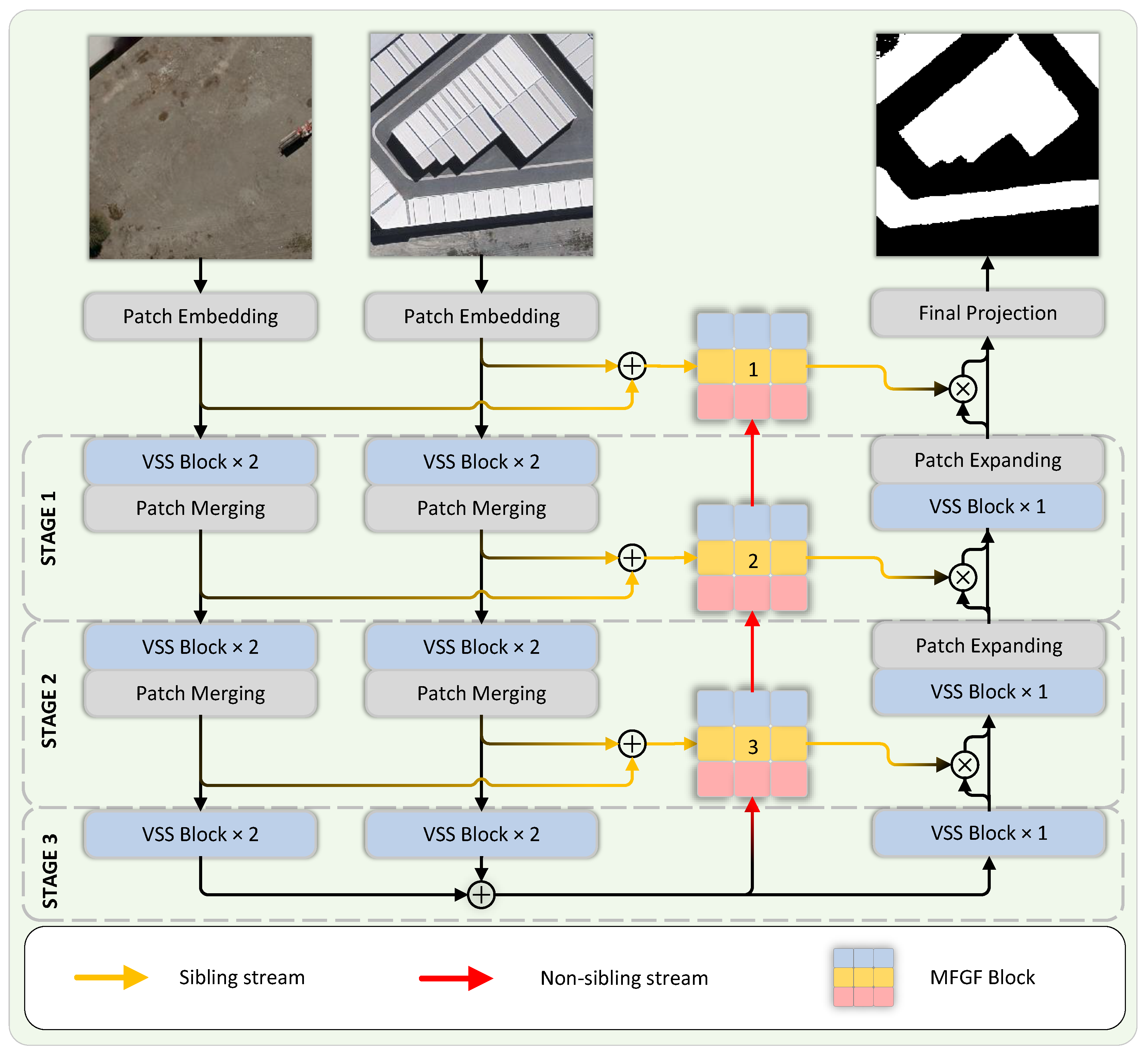
Figure 2.
(a) Architecture of VSS Block. (b) Process of Patch Merging. (c)&(d) Comparison of Self-attention & Cross-Scan.
Figure 2.
(a) Architecture of VSS Block. (b) Process of Patch Merging. (c)&(d) Comparison of Self-attention & Cross-Scan.
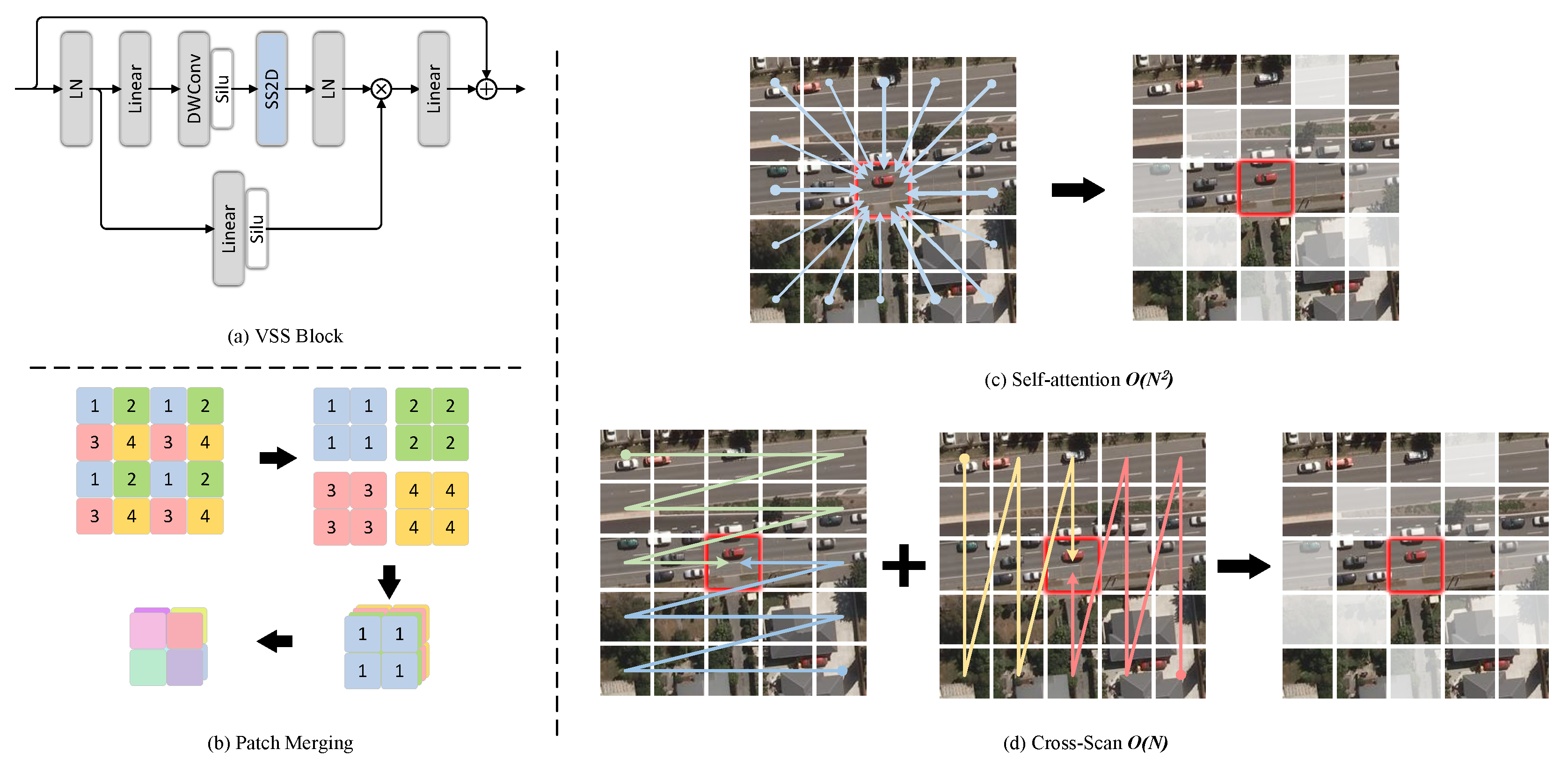
Figure 3.
Architecture of MFGF module.
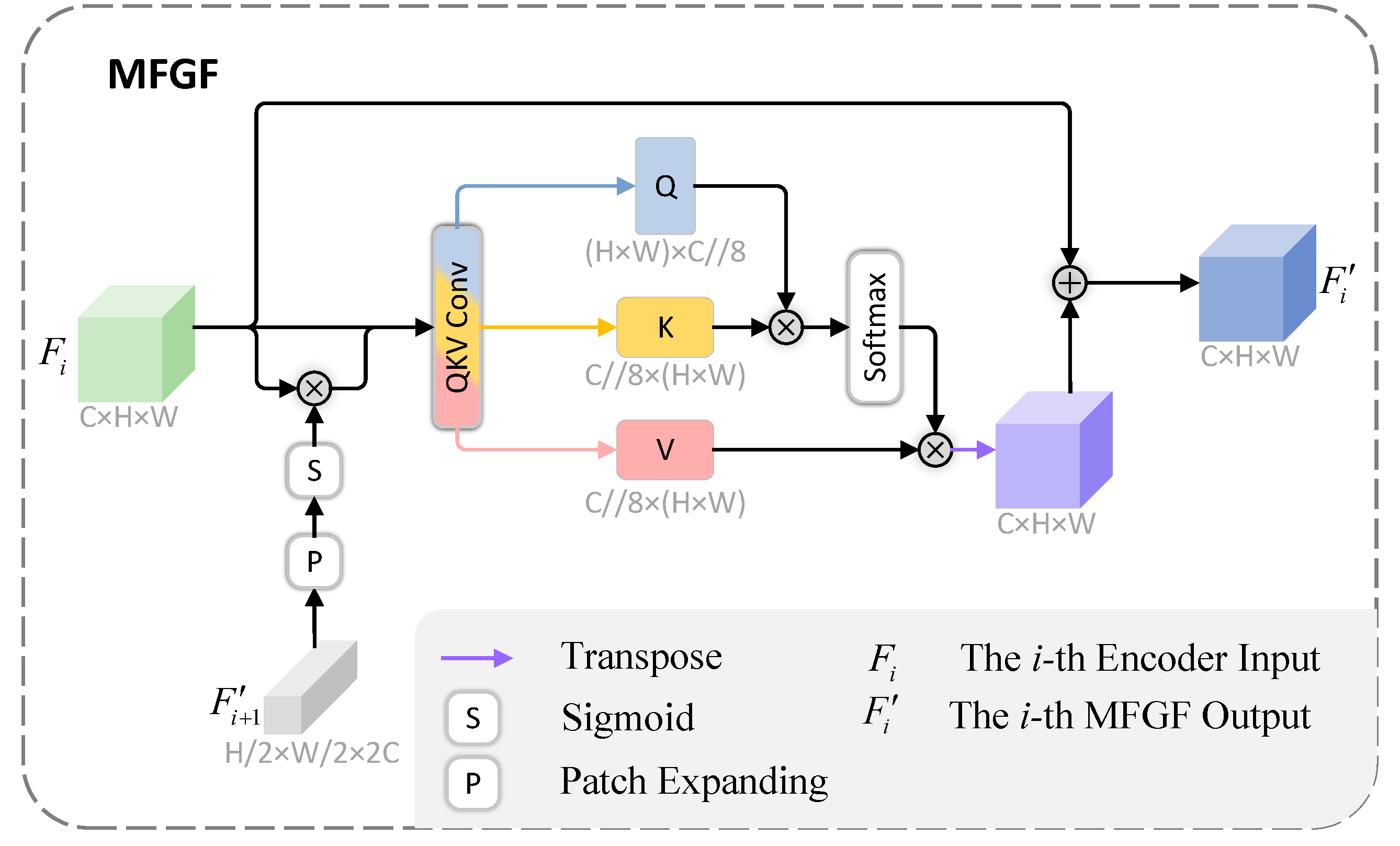
Figure 4.
Qualitative and quantitative analyses of missed detection and false detection.
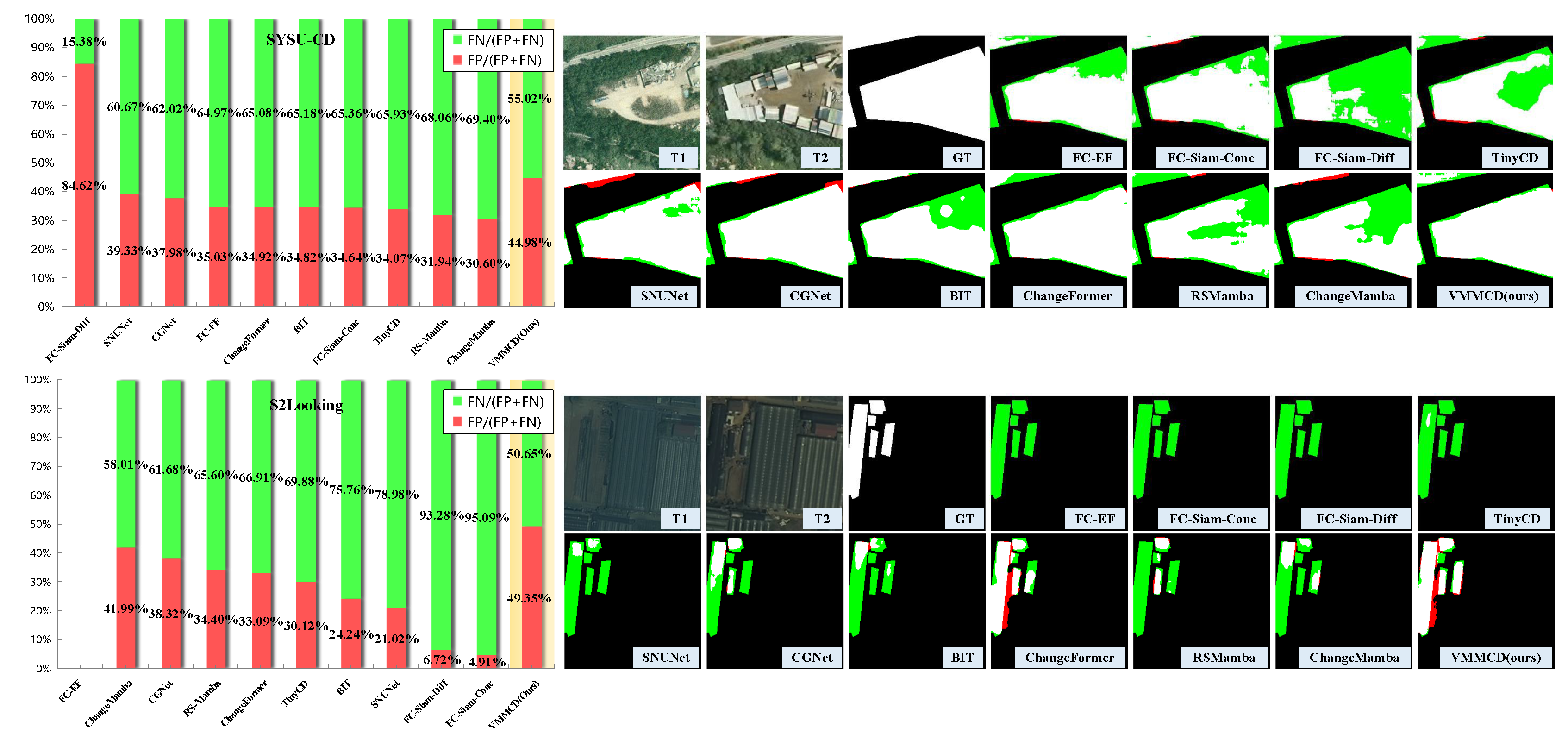
Figure 5.
Visualization results of different models on SYSU-CD[52]. TP (white), TN (black), FP (red), and FN (green).
Figure 5.
Visualization results of different models on SYSU-CD[52]. TP (white), TN (black), FP (red), and FN (green).
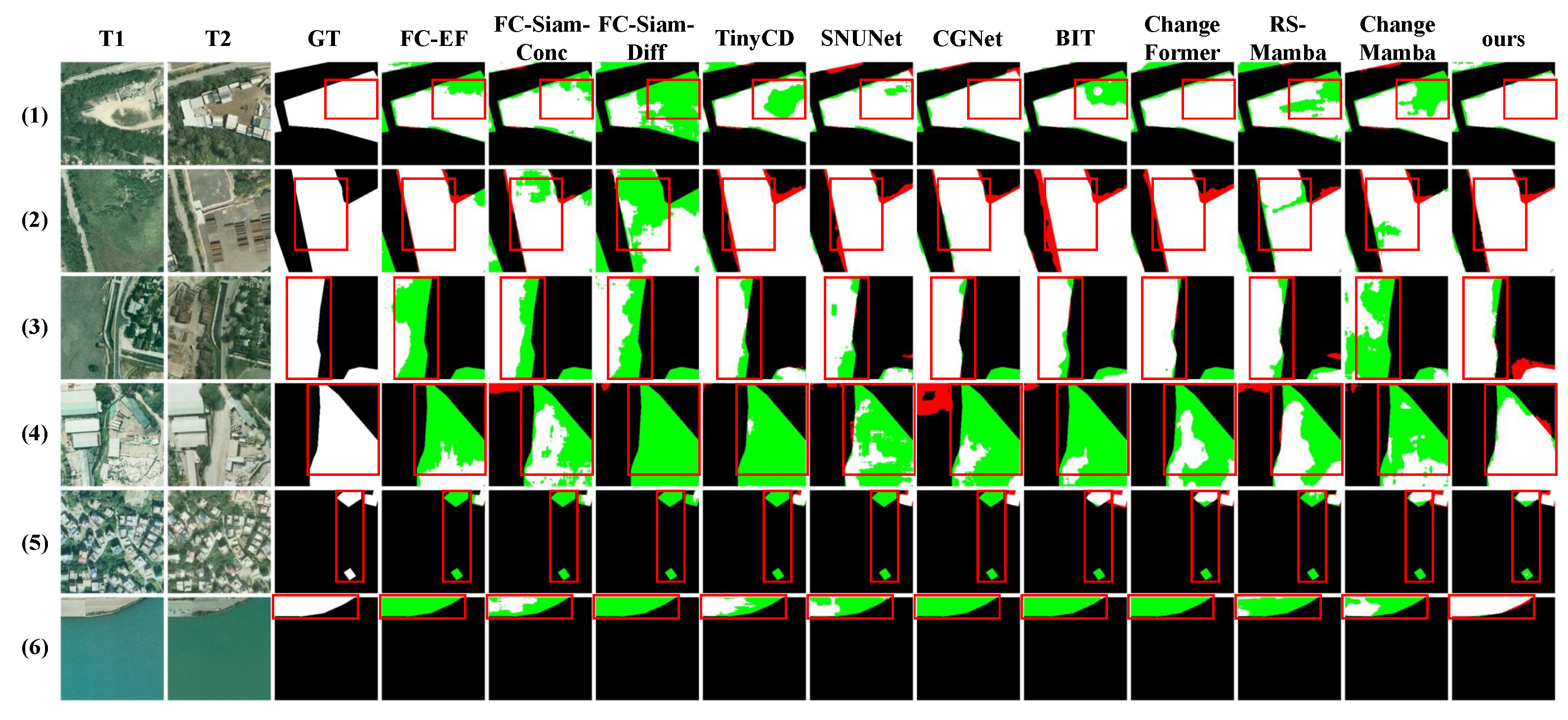
Figure 6.
Visualization results of different models on WHU-CD[53].
Figure 6.
Visualization results of different models on WHU-CD[53].
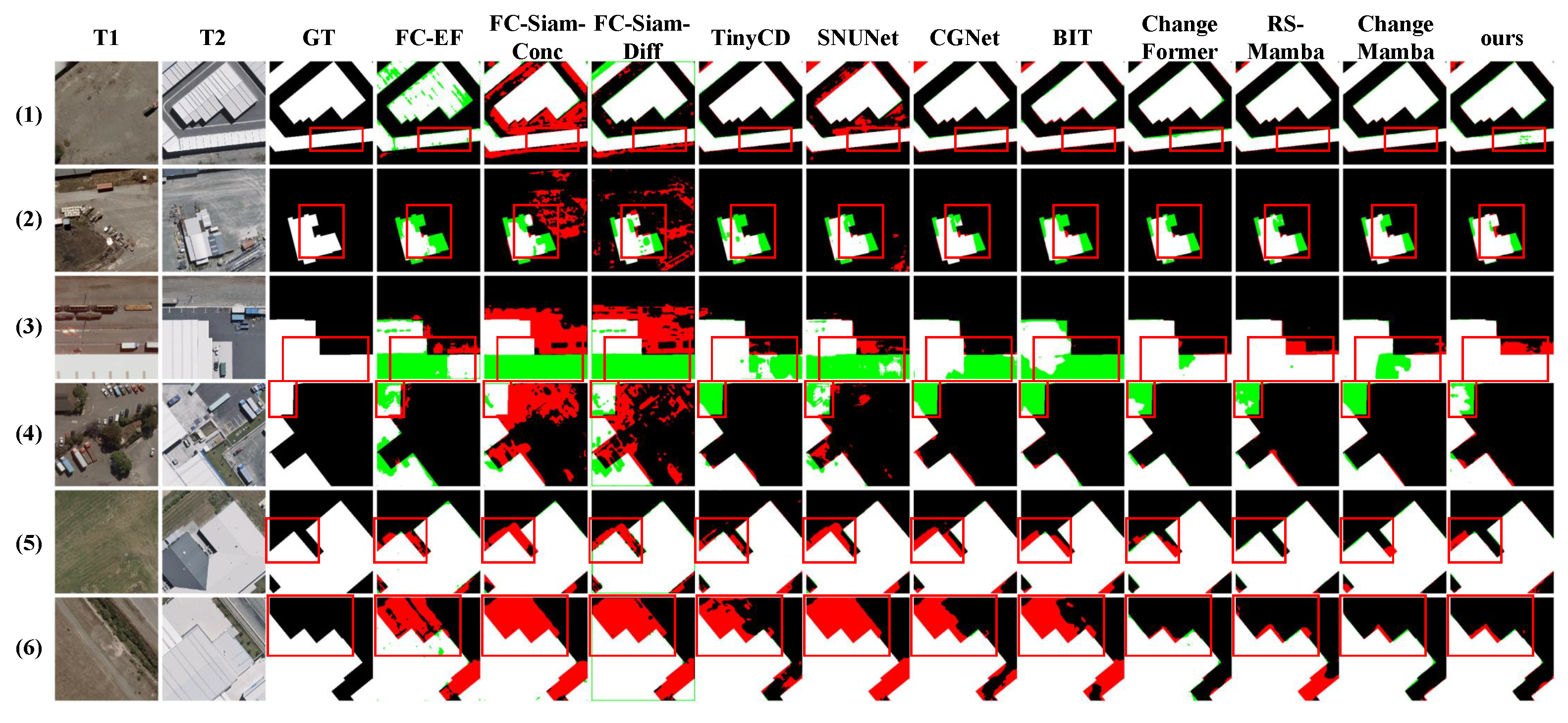
Figure 7.
Visualization results of different models on S2Looking[54].
Figure 7.
Visualization results of different models on S2Looking[54].
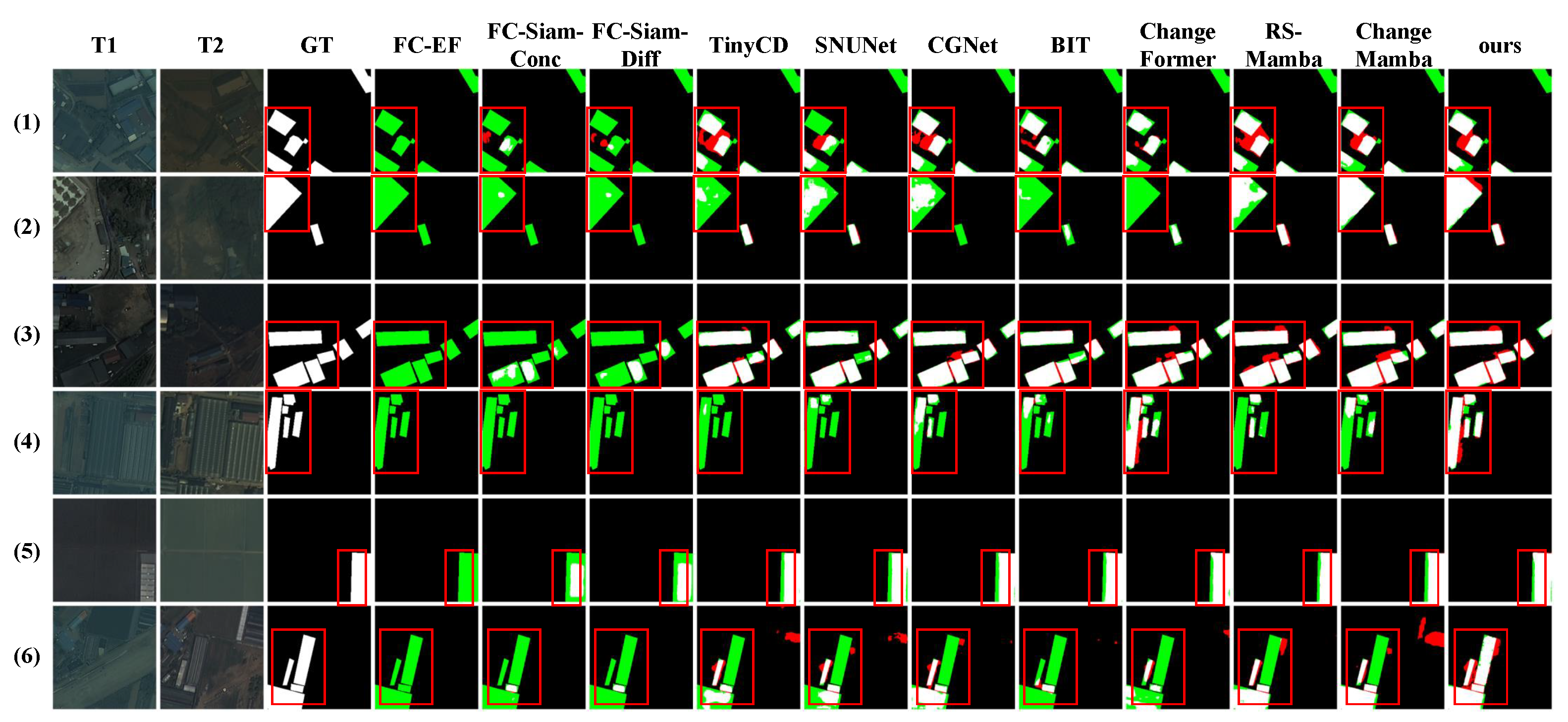
Figure 8.
Visualization of the feature maps at different resolutions and the final binary output.
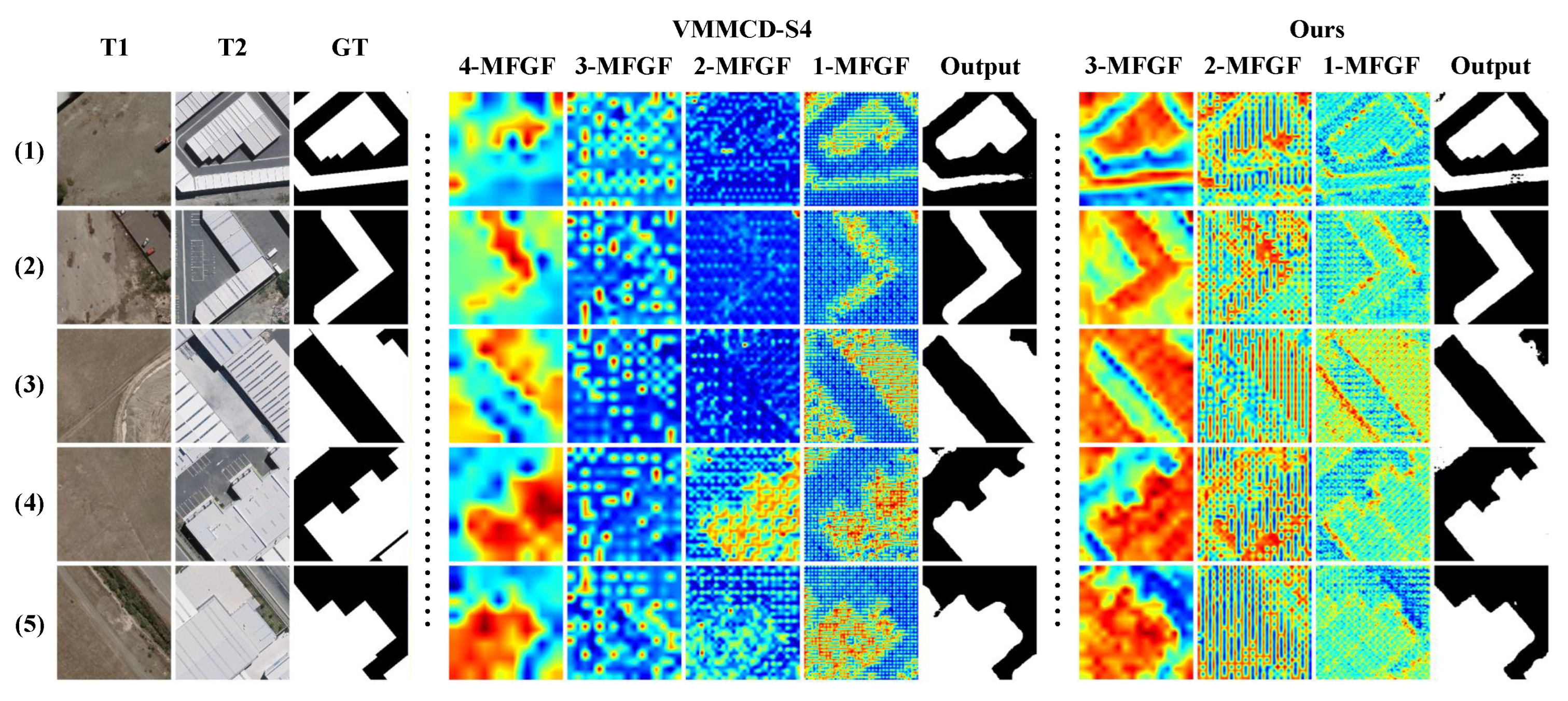
Figure 9.
Visualization results of different MFGF settings on SYSU-CD.
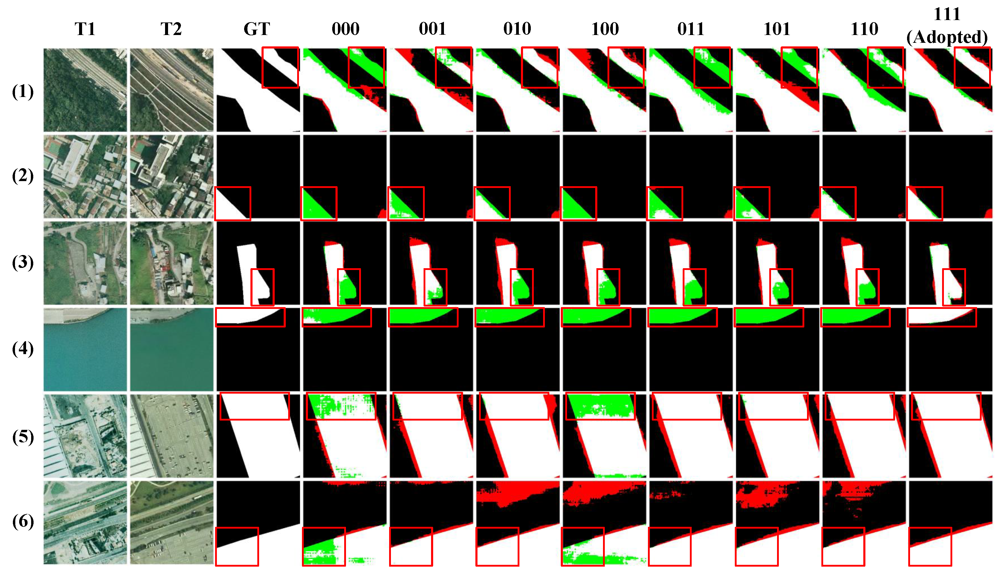

Table 1.
A comparison with other SOTA Change Detection methods on SYSU-CD, WHU-CD, S2Looking. The first, second, and third places are highlighted in red, blue, and black, respectively. Among the metrics, and are the most compelling.
Table 1.
A comparison with other SOTA Change Detection methods on SYSU-CD, WHU-CD, S2Looking. The first, second, and third places are highlighted in red, blue, and black, respectively. Among the metrics, and are the most compelling.
| Type | Method | SYSU-CD[52] | WHU-CD[53] | S2Looking[54] | |||||||||
|---|---|---|---|---|---|---|---|---|---|---|---|---|---|
| Pre. / Rec. / F1 / IoU | Pre. / Rec. / F1 / IoU | Pre. / Rec. / F1 / IoU | |||||||||||
| CNN-based | FC-EF[11] | 80.22 | 68.62 | 73.97 | 58.69 | 74.56 | 73.94 | 74.25 | 59.05 | - | - | - | - |
| FC-Siam-Conc[11] | 81.44 | 69.93 | 75.25 | 60.32 | 38.47 | 84.25 | 52.82 | 35.89 | 84.16 | 21.53 | 34.29 | 20.69 | |
| FC-Siam-Diff[11] | 40.54 | 78.95 | 53.57 | 36.58 | 40.54 | 78.95 | 53.57 | 36.58 | 80.70 | 23.14 | 35.97 | 21.93 | |
| TinyCD[16] | 85.84 | 75.80 | 80.51 | 67.38 | 89.62 | 88.44 | 89.03 | 80.22 | 72.47 | 53.15 | 61.32 | 44.22 | |
| SNUNet[17] | 83.31 | 76.39 | 79.70 | 66.25 | 80.79 | 87.03 | 83.80 | 72.11 | 75.49 | 45.05 | 56.43 | 39.30 | |
| CGNet[41] | 85.60 | 78.45 | 81.87 | 69.30 | 90.78 | 90.21 | 90.50 | 82.64 | 70.18 | 59.38 | 64.33 | 47.41 | |
| Transformer-based | BIT[27] | 83.22 | 72.60 | 77.55 | 63.33 | 84.62 | 88.00 | 86.28 | 75.87 | 75.35 | 49.44 | 59.71 | 42.56 |
| ChangeFormer[42] | 86.47 | 77.42 | 81.70 | 69.06 | 95.58 | 89.83 | 92.62 | 86.25 | 73.33 | 57.62 | 64.54 | 47.64 | |
| Mamba-based | RS-Mamba[39] | 85.38 | 73.27 | 78.86 | 65.10 | 93.70 | 91.08 | 92.37 | 85.83 | 71.49 | 56.80 | 63.30 | 46.31 |
| ChangeMamba[40]* | 88.79 | 77.74 | 82.89 | 70.79 | 91.92 | 92.36 | 94.03 | 88.73 | 68.59 | 61.25 | 64.71 | 47.84 | |
| VMMCD(ours) | 84.76 | 81.97 | 83.35 | 71.45 | 93.84 | 91.23 | 92.52 | 86.08 | 65.45 | 64.86 | 65.16 | 48.32 | |
* The method proposed in our paper employs Mamba-small, thus it is compared here with MambaBCD-Small, which is of a similar Mamba magnitude. Even when compared with MambaBCD-Base, proposed method still outperforms it on both SYSU-CD and S2Looking datasets.
Table 2.
A comparison with other SOTA Change Detection methods on model efficiency. We report GFlops, the number of parameters(in millions), and inference fps(in image pairs per second), as well as the and on SYSU-CD. The shape input image is resized to .
Table 2.
A comparison with other SOTA Change Detection methods on model efficiency. We report GFlops, the number of parameters(in millions), and inference fps(in image pairs per second), as well as the and on SYSU-CD. The shape input image is resized to .
| Type | Method | GFlops | Params | fps | SYSU-CD | |
|---|---|---|---|---|---|---|
| (M) | (pair/s) | F1 / IoU | ||||
| FC-EF[11] | 3.24 | 1.35 | 160.26 | 73.97 | 58.69 | |
| FC-Siam-Conc[11] | 4.99 | 1.55 | 119.75 | 53.57 | 36.58 | |
| FC-Siam-Diff[11] | 4.39 | 1.35 | 122.77 | 75.25 | 60.32 | |
| TinyCD[16] | 1.45 | 0.29 | 85.47 | 80.51 | 67.38 | |
| SNUNet[17] | 11.73 | 3.01 | 67.46 | 79.70 | 66.25 | |
| CGNet[41] | 87.55 | 38.98 | 74.70 | 81.87 | 69.30 | |
| BIT[27] | 26.00 | 11.33 | 62.82 | 77.55 | 63.33 | |
| ChangeFormer[42] | 202.79 | 41.03 | 58.58 | 81.70 | 69.06 | |
| RS-Mamba[39] | 18.33 | 42.30 | 22.58 | 78.86 | 65.10 | |
| ChangeMamba[40] | 28.70 | 49.94 | 16.89 | 82.89 | 70.79 | |
| VMMCD(ours) | 4.51 | 4.93 | 73.05 | 83.35 | 71.45 | |
Table 3.
Ablation on different backbone networks. We report the and scores of the model on SYSU-CD under some different backbone network settings, including 3 CNN-based backbones and 1 ViT-based backbone.
Table 3.
Ablation on different backbone networks. We report the and scores of the model on SYSU-CD under some different backbone network settings, including 3 CNN-based backbones and 1 ViT-based backbone.
| Backbone | GFlops | Params | SYSU-CD | |
|---|---|---|---|---|
| (M) | F1 / IoU | |||
| VGG16[56] | 50.41 | 18.62 | 75.92 | 61.19 |
| ResNet18[57] | 5.49 | 13.21 | 78.50 | 64.61 |
| EfficientNet-B4[58] | 2.71 | 1.44 | 81.57 | 68.87 |
| Swin-small[59] | 15.27 | 24.61 | 68.85 | 52.50 |
| VMamba-small(Ours) | 4.51 | 4.93 | 83.35 | 71.45 |
Table 4.
Ablation on model magnitude. We report the and scores of the model on SYSU-CD under different model magnitude, including 2 scenarios of dimensions in the S3 model and S4 model.
Table 4.
Ablation on model magnitude. We report the and scores of the model on SYSU-CD under different model magnitude, including 2 scenarios of dimensions in the S3 model and S4 model.
| Model | Dims | SYSU-CD | |
|---|---|---|---|
| F1 / IoU | |||
| VMMCD-S4 | OOM | ||
| 80.42 | 67.25 | ||
| 80.23 | 66.98 | ||
| VMMCD-S3 | 80.49 | 67.36 | |
| (Ours) | 81.12 | 68.24 | |
| 80.25 | 67.02 | ||
Table 5.
Ablation on different numbers of MFGF layers. We report the and scores of the model on SYSU-CD under some different MFGF settings, including 8 scenarios in the S3 model and 2 scenarios in the S4 model.
Table 5.
Ablation on different numbers of MFGF layers. We report the and scores of the model on SYSU-CD under some different MFGF settings, including 8 scenarios in the S3 model and 2 scenarios in the S4 model.
| Model | MFGF | SYSU-CD | ||||
|---|---|---|---|---|---|---|
| 1 | 2 | 3 | 4 | F1 / IoU | ||
| VMMCD-S4 | × | × | × | × | 81.88 | 69.33 |
| √ | √ | √ | √ | 82.63 | 70.41 | |
| VMMCD-S3 | × | × | × | - | 82.36 | 70.01 |
| × | × | √ | - | 82.98 | 70.90 | |
| × | √ | × | - | 82.70 | 70.50 | |
| √ | × | × | - | 82.83 | 70.69 | |
| × | √ | √ | - | 83.00 | 70.94 | |
| √ | × | √ | - | 82.99 | 70.92 | |
| √ | √ | × | - | 83.13 | 71.13 | |
| √ | √ | √ | - | 83.35 | 71.45 | |
Table 6.
Ablation on the coefficient of the loss function.
| SYSU-CD | WHU-CD | S2Looking | ||||
|---|---|---|---|---|---|---|
| F1 / IoU | F1 / IoU | F1 / IoU | ||||
| 0 | 83.34 | 71.44 | 92.45 | 85.97 | 64.83 | 47.97 |
| 0.1 | 83.30 | 71.38 | 92.47 | 86.00 | 65.18 | 48.35 |
| 0.2 | 83.35 | 71.45 | 92.52 | 86.08 | 65.16 | 48.32 |
| 0.3 | 83.26 | 71.32 | 92.50 | 86.04 | 65.07 | 48.22 |
| 0.5 | 83.25 | 71.30 | 92.50 | 86.05 | 64.90 | 48.03 |
| 1 | 83.23 | 71.28 | 92.59 | 86.20 | 65.21 | 48.38 |
Disclaimer/Publisher’s Note: The statements, opinions and data contained in all publications are solely those of the individual author(s) and contributor(s) and not of MDPI and/or the editor(s). MDPI and/or the editor(s) disclaim responsibility for any injury to people or property resulting from any ideas, methods, instructions or products referred to in the content. |
© 2025 by the authors. Licensee MDPI, Basel, Switzerland. This article is an open access article distributed under the terms and conditions of the Creative Commons Attribution (CC BY) license (https://creativecommons.org/licenses/by/4.0/).
Copyright: This open access article is published under a Creative Commons CC BY 4.0 license, which permit the free download, distribution, and reuse, provided that the author and preprint are cited in any reuse.


