Submitted:
02 April 2025
Posted:
03 April 2025
You are already at the latest version
Abstract
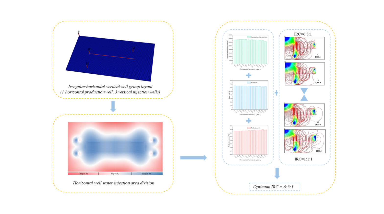
As conventional oil resources decline, optimizing the development of tight reservoirs has become critical for sustaining production. Horizontal wells with artificial fractures offer a promising solution, but improper water injection often leads to uneven waterflooding, particularly in irregular horizontal-vertical well systems—a common challenge in fields like China’s Fuxian oilfield. This study tackles this issue by introducing a practical and effective method to optimize water injection flow rates, significantly enhancing oil recovery in such complex well patterns. Through advanced numerical modeling and three-dimensional flow visualization, we analyze sweep efficiency and water breakthrough risks, categorizing the horizontal well’s drainage area into three distinct regions, each requiring tailored injection rates. Using a representative model with one horizontal well and three vertical wells, we demonstrate that adjusting the flow rate ratio among injectors to 6:3:1 (instead of a uniform 1:1:1) boosts cumulative oil production by an additional 2997.6 m³. These findings provide field engineers with a actionable strategy to improve waterflooding efficiency, directly increasing recoverable reserves and economic viability in tight reservoirs. The proposed approach has immediate relevance for oilfield operations, offering a scalable solution to maximize recovery in similar unconventional reservoirs worldwide.
Keywords:
tight reservoirs
; water injection optimization
; horizontal-vertical well systems
; numerical simulation
; sweep efficiency
1. Introduction
As high-quality and easily exploitable oil resources decline, tight reservoirs have become an important alternative to ensure a continued supply of crude oil [1,2]. Horizontal wells with volume fracturing stimulation are effective technologies for developing tight reservoirs [3]. The use of horizontal wells significantly increases oil production that cannot be achieved through a single vertical well. These wells are intersected by artificial fractures that provide a more efficient flow path for crude oil. However, as development progresses, the oil production of horizontal wells consistently declines with the depletion of formation pressure [4]. To replenish formation energy, petroleum engineers have proposed a series of technologies, including waterflooding, gas flooding, water-alternating-gas (WAG) flooding, water injection huff-n-puff, and gas huff-n-puff [5]. Numerous laboratory experiments and numerical simulations have provided substantial evidence that gas injection, particularly CO2 injection, is a promising enhanced oil recovery (EOR) method due to its favorable attributes, such as high injection capacity and miscibility with oil [6,7]. However, due to the high cost of CO2 sources, water injection remains the most commonly used method.
Water flooding is an effective and cost-efficient technique to enhance oil recovery following primary production in conventional reservoirs. However, significant reservoir heterogeneity caused by natural and artificial fractures often results in low sweep efficiency of injected water in tight reservoirs [8]. To recover more oil through water flooding, researchers primarily focus on optimizing well patterns [9,10]. The diamond-shaped inverted nine-spot well pattern has been shown to be superior to other well patterns in developing fractured tight reservoirs. However, well patterns in oil fields are often irregular [11,12,13]. A typical irregular horizontal and vertical combined well group from the Fuxian oilfield (Ordos Basin, China) is shown in Figure 1. The newly drilled horizontal well serves as both a production and an exploratory well for understanding the area's geology. Consequently, the spacing between newly drilled horizontal wells is relatively large. Meanwhile, there are typically only 1 to 3 water injection wells around a horizontal well due to cost constraints. Additionally, it is impractical to modify the well pattern by drilling new wells in the current era of low oil prices. Therefore, determining suitable injection parameters to improve oil recovery under the existing irregular well patterns is crucial.
According to the available literature in this field, flow rates of different vertical injectors are typically kept the same within a well group. However, flow rates of different vertical injectors should not be uniform in irregular well groups due to the varying relative positions of vertical injectors and horizontal producers [14,15]. To the best of our knowledge, limited literature has focused on the optimization of flow rates in irregular well groups. Therefore, this study employs streamline simulation and 3D visualization technology to optimize the injection parameters of irregular well groups.
The findings of this research have significant practical implications for the development of tight reservoirs, particularly in mature fields with irregular well patterns. By optimizing injection rates based on spatial relationships between wells, this approach can enhance sweep efficiency without the need for costly infrastructure changes, making it economically viable for operators in low-price oil environments. Furthermore, the methodology can be extended to other unconventional reservoirs, such as shale or low-permeability formations, where uneven fluid distribution is a persistent challenge. From a broader perspective, this work contributes to sustainable hydrocarbon recovery by maximizing resource utilization and delaying well abandonment, thereby reducing the environmental footprint per unit of oil produced.
In this paper, twenty-two cases with varying relative positions of vertical injectors and horizontal producers were initially studied. Based on the simulation results, the controlling area of the horizontal well was divided into three regions where vertical injectors should perform different flow rates. Subsequently, a typical irregular well group with one horizontal well and three vertical wells was studied to determine the flow rate ratio between the injectors from different regions. Finally, analyses of the streamline simulation were conducted to illustrate the mechanism behind the difference in sweep efficiency caused by varying flow rate ratios between the injectors.
2. Reservoir Modeling
2.1. Modeling of a Combined Well Network of One-Injection-one-Production Water Straight
To optimize the injection parameters for the horizontal-straight well group, a conceptual model consisting of one vertical injection well and one horizontal production well was developed. The governing mathematical model for seepage mechanics is presented as follows:
- (1)
- Seepage model of fluid in Region I:
Fluid flow in Region I comprises three components: (1) Darcy flow through the artificial main fracture along the x-direction, (2) Darcy flow from the fracture in Region II into the artificial main fracture along the y-direction, and (3) fluid transfer from the matrix in Region II into the artificial main fracture along the y-direction. The oil and water phase continuity equations governing fluid flow from the artificial main fracture to the wellbore are expressed as Equation (1-2):
In Equation [1,2], variables and denote the oil-phase and water-phase pressures (MPa) in the Region II fracture grid at the Region II-I interface, respectively.
The governing equations for matrix-to-fracture fluid transfer toward the artificial main fractures are:
Substituting Equation (3) into Equations (1) and (2) yields the continuity equation for fluid flow in Region I:
- (2)
- Seepage model of fluid in Region II:
Region II represents a dual-porosity system characterized by multidirectional fluid flow, encompassing matrix flow in both x- and y-directions within the region, along with fluid transfer from the matrix to fractures. At the Region II-I boundary, y-directional flow occurs from both matrix and fractures in Region II to Region I, while the Region II-III interface exhibits x-directional flow from Region III to Region II through matrix and fracture networks. Similarly, y-directional transfer takes place from Region IV to Region II at their shared boundary. The governing differential equations describing this coupled matrix-fracture flow system, including the oil-water phase behavior in fractures, are expressed as Equation (6-7):
In the Equation, the phase pressures are defined as follows:
and : oil-phase and water-phase pressures (MPa) in the Region III fracture grid at the Region III-II interface
and : corresponding phase pressures (MPa) in the Region III matrix grid
and : oil-water phase pressures (MPa) in the Region IV fracture grid at the Region IV-II boundary
and : phase pressures (MPa) in the Region IV matrix grid at the same boundary
The governing differential equations for oil-water two-phase flow in the matrix system are:
The mass transfer equation governing matrix-fracture crossflow is expressed as:
By substituting Equation (9) into the governing equations (6) -(8), we derive the coupled system of oil-water phase flow equations for the fracture network:
Seepage equations for the oil and water phases in the matrix:
- (3)
- Seepage model of fluid in Region III:
Differential equations of seepage for the oil phase and water phase in the matrix:
The governing differential equations for oil-water two-phase flow in the matrix are given by Equations (13) and (14):
The governing differential equations for oil-water two-phase flow in the fracture network are given by Equations (15) and (16):
Among these equations, the equation governing the cross-flow phenomenon from the matrix to the fractures is as follows:
- (4)
- Seepage model of fluid in Region IV:
Fluid flow in Region IV consists of y-directional matrix flow and y-directional matrix-fracture transfer to Region II, with the governing differential equations for this coupled matrix-fracture system expressed as follows:
The governing differential equations describing oil-water two-phase flow in the matrix system are given by Equations (18) and (19):
The governing differential equations for oil-water two-phase flow in the fracture system are given by Equations (20) and (21):
Among these, the equation that describes the mechanism of cross-flow from the matrix to the fractures is as follows:
- (5)
- The initial and boundary condition equations:
The initial and boundary condition equations are displayed as follows:
initial conditional equation:
boundary condition equation:
Based on the geological characteristics of the Huangjialing block in Fu County and the average size of the water-straight combined well group, a conceptual flow line model, featuring one straight well for water injection and one horizontal well for oil production, was also established, as shown in Figure 2. The one-injection-one-production water-straight joint well group model with varying relative positions was then simulated to investigate the water injection pattern within the network.
As shown in Figure 2, the conceptual model for a single injection and extraction process displays both centrosymmetric and axisymmetric distributions. Therefore, only a subset of the regions, labeled A, B, C, and D, requires a detailed investigation. To demonstrate this, Region A is selected for consideration. By discretizing the fracturing-reforming and non-fracturing-reforming areas and assigning the injection wells Ii-j to the corresponding regions, 22 conceptual models of the one-injection-one-mining process with various relative positions of horizontal and vertical wells were generated. The matrix of I is presented in Equation (1). All wells labeled I1-1 to I6-41 in Equation (1) correspond to potential injection well locations. However, each simulation case adheres to a one-injection-one-production configuration; only one injection well is active at any given time, while the horizontal production well remains fixed. This controlled approach enables a systematic comparison of water injection efficiency across 22 distinct injection well locations, isolating the influence of spatial configuration on development performance.
Hydraulic fracturing is conducted around the horizontal well. The post-fracturing formation can be characterized by a combination of fracture systems and matrix. The conceptual model is depicted in Figure 3.
As shown in Figure 3, the conceptual model can be divided into four regions (I, II, III, and IV). Due to their centrosymmetric nature, only one region (Region I) was selected to study the injection parameters of the horizontal-straight well group. Region I comprises both the fracture system and the matrix system. The water injection well Wi was positioned in the conceptual model. A total of 22 one-injection-one-production configurations with different relative positions of horizontal and straight wells were obtained.
2.2. Establishment of the One-Injection-One-Production Streamline Model
Two common grid division methods include center-block grids and corner-point grids [16,17]. The former is simpler and more accurate for radial geological simulations, while the latter better simulates complex features like faults and pinch-outs [18]. For the conceptual model, corner-point grids enhance streamline distribution accuracy without requiring complex stratigraphic considerations. Therefore, corner-point grids are the most suitable choice for this model. Statistical analysis of the Huangjialing block's water-straight well group determined the model dimensions as 1400 m × 800 m × 40 m. The plane grid was divided into 140 × 80 cells, with a 10 m × 10 m step size. The tight reservoir grid division is illustrated in Figure 4. The reservoir's top depth was measured at 1425 m.
The typical tight reservoir parameters of the Fuxian Oilfield (Ordos Basin, China) are presented in Table 1. Based on these parameters, the grid properties of the one-injection-one-production conceptual model for this block were determined.
The one-injection-one-production conceptual model for this block was established. Figure 5 illustrates the streamline conceptual model corresponding to I1-1, in which the water injection well is positioned at coordinates (1, 1).
A unified production scheme was applied to simulate the 22 one-injection-one-production models established in Section 2.1, using an injection-production ratio of 1.06 and a simulation duration of 6400 days. The simulation results, evaluated based on the production duration to reach the economic limit daily oil production, cumulative oil production, and streamline distribution in the one-injection-one-production models, are summarized in Table 2.
3. Classification of Water Injection Area
In this study, the economic limit was introduced to facilitate the classification of the water injection area. The economic limit of a horizontal well is defined as the balance between the profits from oil production and the investments in initial costs, personnel management, and equipment maintenance. In the Fuxian oilfield, the economic limit is reached when the oil production rate falls below 3 m3/d. The time at which the production of horizontal wells reaches the economic limit is termed the “limit time.”
Streamline simulations of 22 one-injection-one-production cases were conducted to classify the water injection area in this study. In these cases, the horizontal well was operated for 300 days without energy supplementation, followed by water flooding. The injection-production ratio was set to 1.1:1. To ensure the economic limit could be reached in all models, the simulation period was set to 6100 days. To investigate the effect of different relative locations between vertical and horizontal wells on oil recovery, plane interpolation was performed on the production time, cumulative oil production, and water cut data from 22 streamline models at the economic limit. The results were visualized in 3D using Matplotlib. The simulation results, including limit time, cumulative oil production, and water cut, are presented in Figure 6, Figure 7 and Figure 8.
Statistical analysis of the simulation results revealed that the relative location between the water-injection well and the horizontal well significantly influenced production. As the distance between the vertical well and the fracturing zone decreased, the horizontal well exhibited higher water cut, shorter limit time, and lower cumulative oil production. In the direction perpendicular to the horizontal well, the development effect increased monotonically with the distance between the vertical well and the horizontal wellbore. In the parallel direction, the development effect first decreased and then increased.
The distribution of formation pressure at the end of depletion development significantly influences the water-injection response. As inferred from Figure 9, the injected water can easily sweep the fracturing zone due to the significant reduction in formation pressure within the fracturing zone. Figure 10 illustrates that the streamline is densely distributed perpendicular to the wellbore in the initial period, while the opposite trend is observed at the end of depletion development. However, channeling paths can readily form near the fracturing zone [19]. Therefore, injecting large amounts of water near the fractured zone may result in low oil recovery, while the formation pressure in areas far from the fracturing zone remains high. To enhance the controlled reserves of the horizontal well, it is necessary to improve sweep efficiency through water injection. Additionally, higher water-injection intensity can be applied to enhance oil displacement in areas far from the fracturing zone.
By projecting the economic limit onto a plane (Figure 6) and applying the principle of central symmetry, the classification diagram of water injection regions (Figure 11) was obtained. The region around the horizontal well was divided into three water-injection areas based on the economic limit. Reducing the water injection intensity in region #3 or increasing the volumetric flow rate of injected water in region #1 enhances the effectiveness of water flooding.
4. Water Injection Ratio Coefficient Optimization and Mechanism Analysis
4.1. Water Injection Ratio Coefficient Optimization
As shown in Figure 12, a typical irregular horizontal-vertical well group was established in this section to determine the water injection ratio coefficient for each injection well. To optimize the water injection ratio coefficient, a series of numerical simulations were conducted based on the twelve sets of ratio coefficients (see Table 3). In this numerical simulation, the horizontal well was operated for 300 days without energy supplementation, followed by water flooding for 5800 days at an injection-production ratio of 1.1. Cumulative oil production, water cut, and production rate were used to evaluate the water injection ratio coefficient. The simulation results are presented in Figure 13, Figure 14 and Figure 15.
As shown in Figure 13, the highest cumulative oil production after 6,100 days can be achieved with the water-injection ratio coefficient of combination #4, and the cumulative oil production is 33967.08 m3, which is 2997.6 m3 higher than that the combination #12 with a balanced water-injection ratio. Injection wells in region #1 not only supplemented formation energy but also displaced the remaining oil after the depletion development. So, we can increase the water-injection ratio coefficient of region #1 injection wells to get more oil production. Because the Region #3 is closer to the fracturing area of the horizontal well, the formation energy in this area is severely deficient after depletion development. If excessive water is injected into region #3, water channeling would be occurred along with fractures. It would reduce the sweep efficiency and affect the displacement of the remaining oil. Therefore, the injection intensities in region #3 should be reduced. As shown in Figure 14, the horizontal well reaches the high water cut period (water cut> 60%) till the 6100th days in all the 12 combinations. We can also find from Figure 15 that the production rate in all of the 12 combinations is nearly the same. Therefore, the IRC should be set as 6:3:1 to yield the high oil recovery.
4.2. Mechanism Analysis of Injection Intensities Classification
To investigate the mechanism of injection intensity classification, streamline distributions under 12 water injection ratio coefficients were simulated using FrontSim (see Figure 16). The distribution range of streamlines indicates the effectiveness of water flooding. The density of streamlines correlates with the sweep efficiency of water flooding. Higher streamline density corresponds to greater sweep efficiency [20].
As shown in Figure 16, the distribution of streamlines remains similar across the 12 different water injection ratio coefficients, suggesting that the classification of water injection intensities has minimal impact on the controlled areas of water flooding. In Figure 16(1) and 14(2), streamlines are densely concentrated around I1, indicating that the reservoir displacement around I1 is sufficient under high water injection intensities. However, the streamlines near I2 and I3 are sparsely distributed, implying relatively low sweep efficiency in the water flooding process. In Figure 16(3), 14(4), and 14(5), the streamlines near the horizontal well and water injection wells are densely packed, indicating that sweep efficiency is improved and the water flooding effect is more favorable under these three water injection ratio coefficients. Compared to the other combinations, the streamline distribution in combination 4 (IRC = 6:3:1) is denser in the central area of the horizontal well, suggesting that it effectively supplements energy to the central region and enhances the water injection development process. In combination #12, with balanced water injection, the controlled area of I1 is smaller than in combination #4. Moreover, the water flooding front of I1 in combination #12 is positioned far from the horizontal well at day 6100, indicating that the balanced water injection method yields less effective results.
Combinations #1 (IRC = 7.5:1.5:1), #4 (IRC = 6:3:1), and #12 (IRC = 1:1:1) were selected to demonstrate the streamline distribution at days 2800 and 4200 (see Figure 17). In combination #1, the water flooding front of I1 reaches the horizontal well by day 2800. However, by day 4200, water channeling in I1 results in a rapid increase in water cut. The water injection volumes for each well in combination #12 are nearly identical, but because I2 and I3 are located close to the fracturing zone and formation energy in these areas decreases significantly after depletion development, a large pressure gradient forms after water injection, causing the water injection fronts of wells I2 and I3 to reach the horizontal well quickly. As a result, the oil cannot be displaced effectively. Additionally, due to insufficient water injection at well I1, the water flooding front advances slowly, leading to sparse streamlines in the middle of the horizontal well and failing to effectively supplement the formation energy in this area. In combination #4, the water injection ratios for each well are relatively balanced. By day 2800, the water flooding fronts of wells I2 and I3 are near the horizontal well. Moreover, as seen in the streamline distribution at day 4200, the oil saturation around the horizontal well has not significantly decreased, indicating that the injected water effectively displaces crude oil in the reservoir towards the production well without causing water channeling.
5. Conclusions
This study develops a novel classification method for water injection regions in irregular horizontal-vertical well groups, demonstrating that optimized, region-specific water injection strategies can significantly enhance oil recovery compared to conventional balanced injection approaches. Through comprehensive numerical and streamline simulations, we establish three distinct injection regions around horizontal wells, with Region #1 requiring the highest injection intensity and Region #3 the lowest, as validated by the superior performance of the 6:3:1 injection ratio coefficient (achieving 2997.6 m³ cumulative production after 6100 days). These findings directly address our research question by proving that classification based on post-depletion pressure and flow field distributions can effectively guide waterflooding strategies to enhance formation energy while preventing premature water breakthrough. The practical implications are substantial, offering field operators a scientifically-grounded framework for designing injection schemes in irregular well patterns, particularly in similar heterogeneous reservoirs. However, we acknowledge that our current model assumes homogeneous reservoir conditions, and future work should incorporate reservoir heterogeneity, real-time dynamic adjustment of injection ratios, and potential integration with machine learning for more complex field applications. This research provides both theoretical advancements and practical methodologies that can be immediately implemented in field operations while paving the way for more sophisticated, data-driven approaches to waterflood optimization in various reservoir types.
Author Contributions
Conceptualization, H.Y. and J.Y.; methodology, H.Y and J.Y.; software, H.Q.; formal analysis, S.Y.; investigation, H.Q.; writing—original draft preparation, H.Y. and J.Y; writing—review and editing, J.Y.; supervision, S.Y.; All authors have read and agreed to the published version of the manuscript.
Data Availability Statement
Data are contained within the article.
Conflicts of Interest
The authors declare no conflicts of interest.
References
- Hu, S.; Zhu, R.; Wu, S.; et al. Exploration and development of continental tight oil in China. Petrol. Explor. Dev. 2018, 45, 790–802. [Google Scholar] [CrossRef]
- Tomassi A, de Franco R, Trippetta F. High-resolution synthetic seismic modelling: elucidating facies heterogeneity in carbonate ramp systems[J]. Petrol. Geosci. , 2025, 31, 1, petgeo2024-047. [CrossRef]
- Yekeen, N.; Padmanabhan, E.; Idris, A. K.; et al. Nanoparticles applications for hydraulic fracturing of unconventional reservoirs: A comprehensive review of recent advances and prospects. J. Pet. Sci. Eng. 2019, 178, 41–73. [Google Scholar] [CrossRef]
- Yu, H.; Rui, Z.; Chen, Z.; et al. Feasibility study of improved unconventional reservoir performance with carbonated water and surfactant. Energy 2019, 182, 135–147. [Google Scholar] [CrossRef]
- Jackson, M. D.; Vinogradov, J.; Hamon, G.; et al. Evidence, mechanisms and improved understanding of controlled salinity waterflooding part 1: Sandstones. Fuel 2016, 185, 772–793. [Google Scholar] [CrossRef]
- Eyinla, D. S.; Leggett, S.; Badrouchi, F.; et al. A comprehensive review of the potential of rock properties alteration during CO2 injection for EOR and storage. Fuel 2023, 353, 129219. [Google Scholar] [CrossRef]
- Sheng, J. J. Enhanced oil recovery in shale reservoirs by gas injection. J. Nat. Gas Sci. Eng. 2015, 22, 252–259. [Google Scholar] [CrossRef]
- Li Q, Li Q, Wu J, et al. Wellhead stability during development process of hydrate reservoir in the Northern South China Sea: Evolution and mechanism. Processes, 2024, 13 , 1, 40. [CrossRef]
- Li, Y.; Xu, W.; Xiao, F.; et al. Optimization of a development well pattern based on production performance: A case study of the strongly heterogeneous Sulige tight sandstone gas field, Ordos Basin. Nat. Gas Ind. B 2015, 2, 95–100. [Google Scholar] [CrossRef]
- Rongze, Y.; Yanan, B.; Kaijun, W.; et al. Numerical Simulation Study on Diamond-Shape Inverted Nine-Spot Well Pattern. Phys. Procedia 2012, 24, 390–396. [Google Scholar] [CrossRef]
- Kou, Z.; Wang, H.; Alvarado, V.; et al. Method for upscaling of CO2 migration in 3D heterogeneous geological models. J. Hydrol. 2022, 613, 128361. [Google Scholar] [CrossRef]
- Kou, Z.; Zhang, D.; Chen, Z.; et al. Quantitatively determine CO2 geosequestration capacity in depleted shale reservoir: A model considering viscous flow, diffusion, and adsorption. Fuel 2022, 309, 122191. [Google Scholar] [CrossRef]
- Wang, H.; Kou, Z.; Bagdonas, D. A.; et al. Multiscale petrophysical characterization and flow unit classification of the Minnelusa eolian sandstones. J. Hydrol. 2022, 607, 127466. [Google Scholar] [CrossRef]
- Yue, P.; Xie, Z.; Liu, H.; et al. Application of water injection curves for the dynamic analysis of fractured-vuggy carbonate reservoirs. J. Pet. Sci. Eng. 2018, 169, 220–229. [Google Scholar] [CrossRef]
- Strickland, T. A.; Crawford, P. B. Predicted areal sweep efficiency when using horizontal wells in five-spot patterns. Fuel 1991, 70, 1324–1326. [Google Scholar] [CrossRef]
- Abou-Kassem, J. H.; Islam, M. R.; Ali, S. M. F. Petroleum Reservoir Simulation, 2nd ed.; Elsevier: 2020; pp. 65–124. [CrossRef]
- Sepehrnoori, K.; Xu, Y.; Yu, W. EDFM for field-scale reservoir simulation with complex corner-point grids. Dev. Pet. Sci. 2020, 68, 191–237. [Google Scholar] [CrossRef]
- Xu, Y.; Fernandes, B. R. B.; Marcondes, F.; et al. Embedded discrete fracture modeling for compositional reservoir simulation using corner-point grids. J. Pet. Sci. Eng. 2019, 177, 41–52. [Google Scholar] [CrossRef]
- Ishibashi, T.; Watanabe, N.; Tamagawa, T.; et al. Three-dimensional channeling flow within subsurface rock fracture networks suggested via fluid flow analysis in the Yufutsu fractured oil/gas reservoir. J. Pet. Sci. Eng. 2019, 178, 838–851. [Google Scholar] [CrossRef]
- Nelson, R.; Zuo, L.; Weijermars, R.; et al. Applying improved analytical methods for modelling flood displacement fronts in bounded reservoirs (Quitman field, east Texas). J. Pet. Sci. Eng. 2018, 166, 1018–1041. [Google Scholar] [CrossRef]
Figure 1.
Sand thickness distribution of the Chang 81 reservoir in Fuxian oilfield (Ordos Basin, China). illustrating: (1) the irregular well pattern configuration (horizontal production well HW1 and three vertical injection wells V1–V3); (2) spatial heterogeneity of sand body development (thickness range: 8–22 m); (3) the geological setting for streamline simulation.
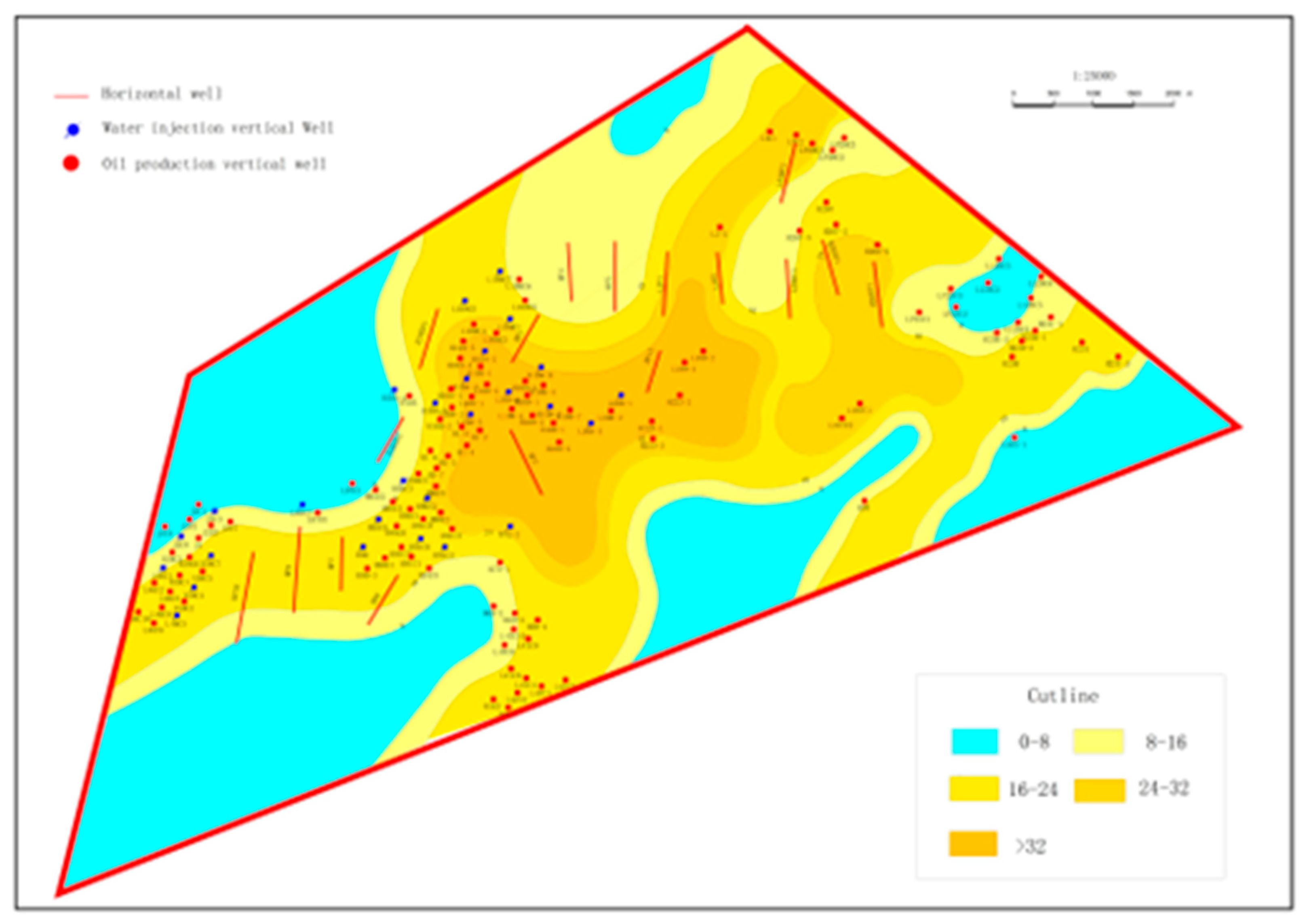
Figure 2.
Conceptual model of one-injection-one-production (1400*800*40).
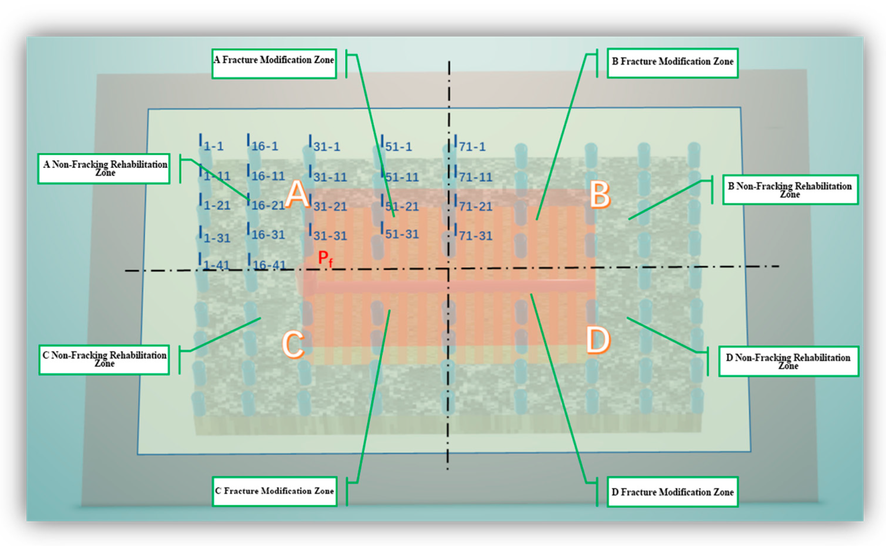
Figure 3.
The conceptual model of one vertical injection well and one horizontal production well.
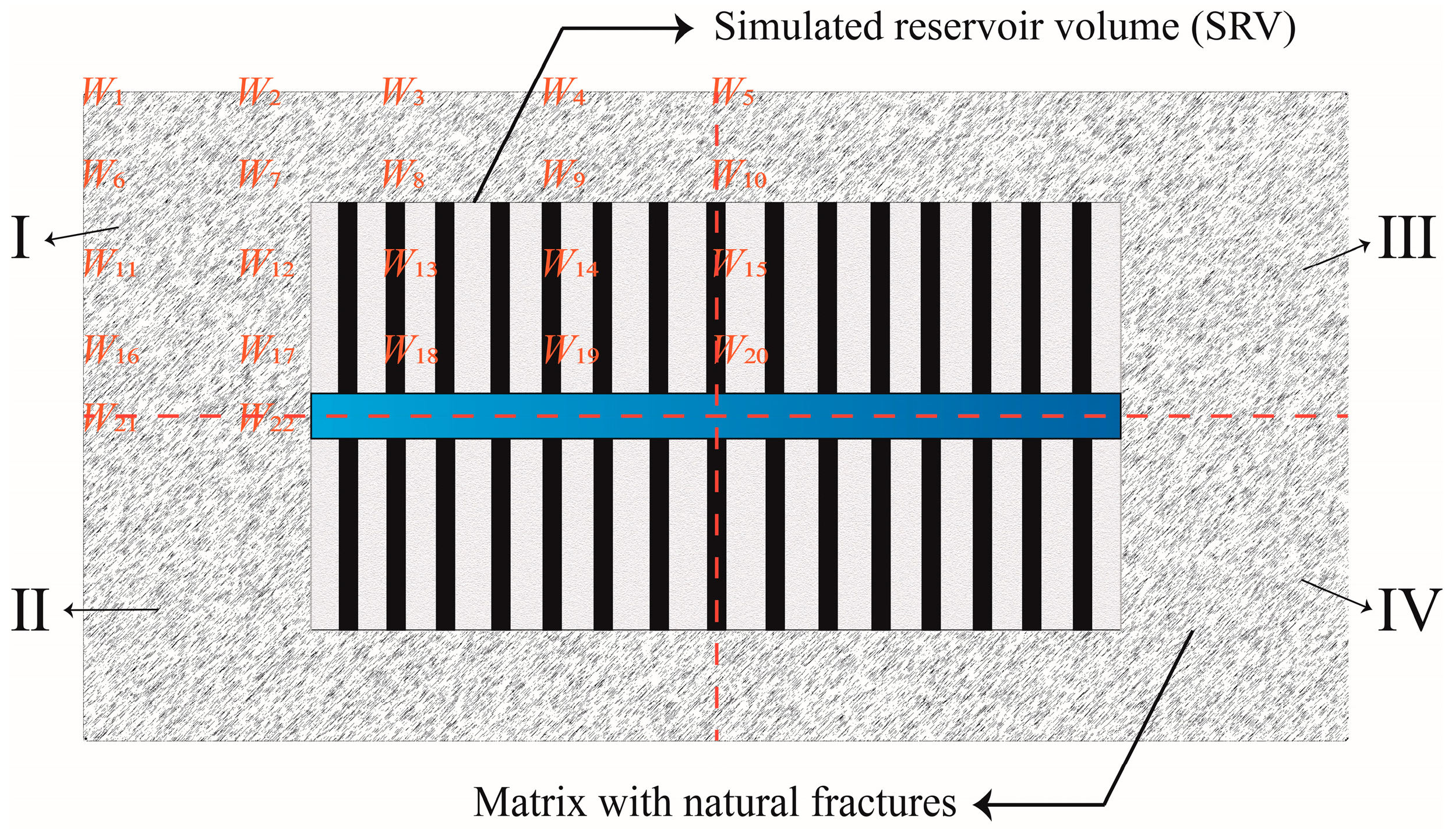
Figure 4.
Mesh generation.
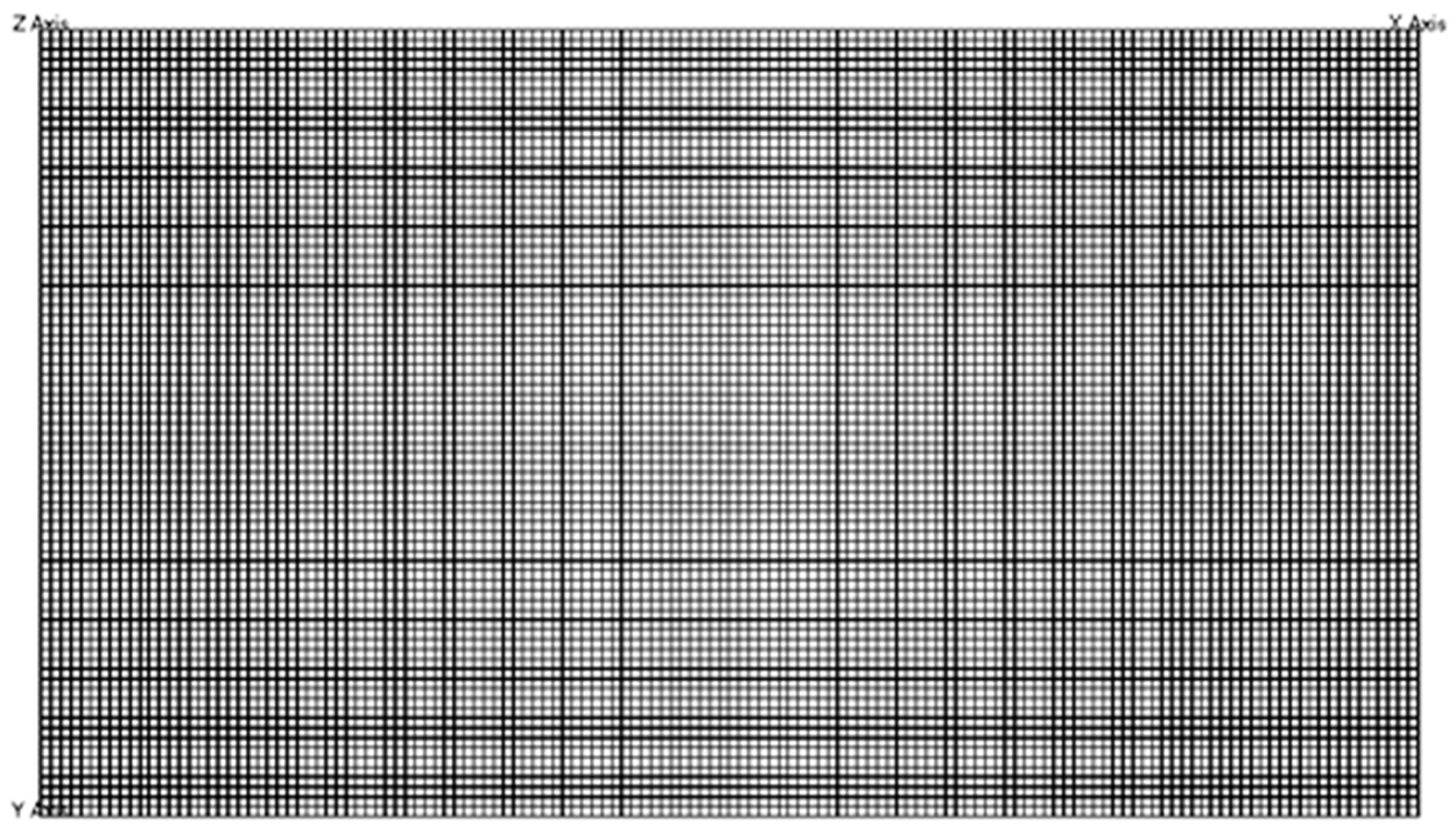
Figure 5.
Conceptual Model of One-Injection-One-Production.
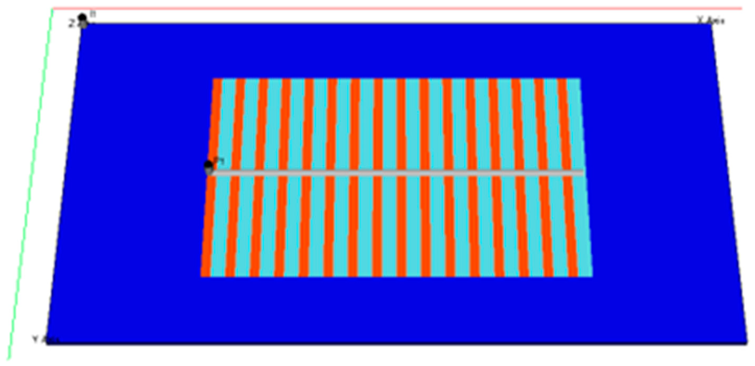
Figure 6.
3D visualization of the limit time (days) for horizontal wells under different relative locations between vertical injection wells and horizontal production wells. The results were obtained from 22 streamline simulations at the economic limit (oil production rate < 3 m³/d). The variables x and y represent the coordinate system relative to the horizontal well orientation.

Figure 7.
3D visualization of the cumulative oil production (m³) at the economic limit for different relative locations between vertical injection wells and horizontal production wells. The results were derived from streamline simulations with an injection-production ratio of 1.1:1. The variables x and y represent the coordinate system relative to the horizontal well orientation.
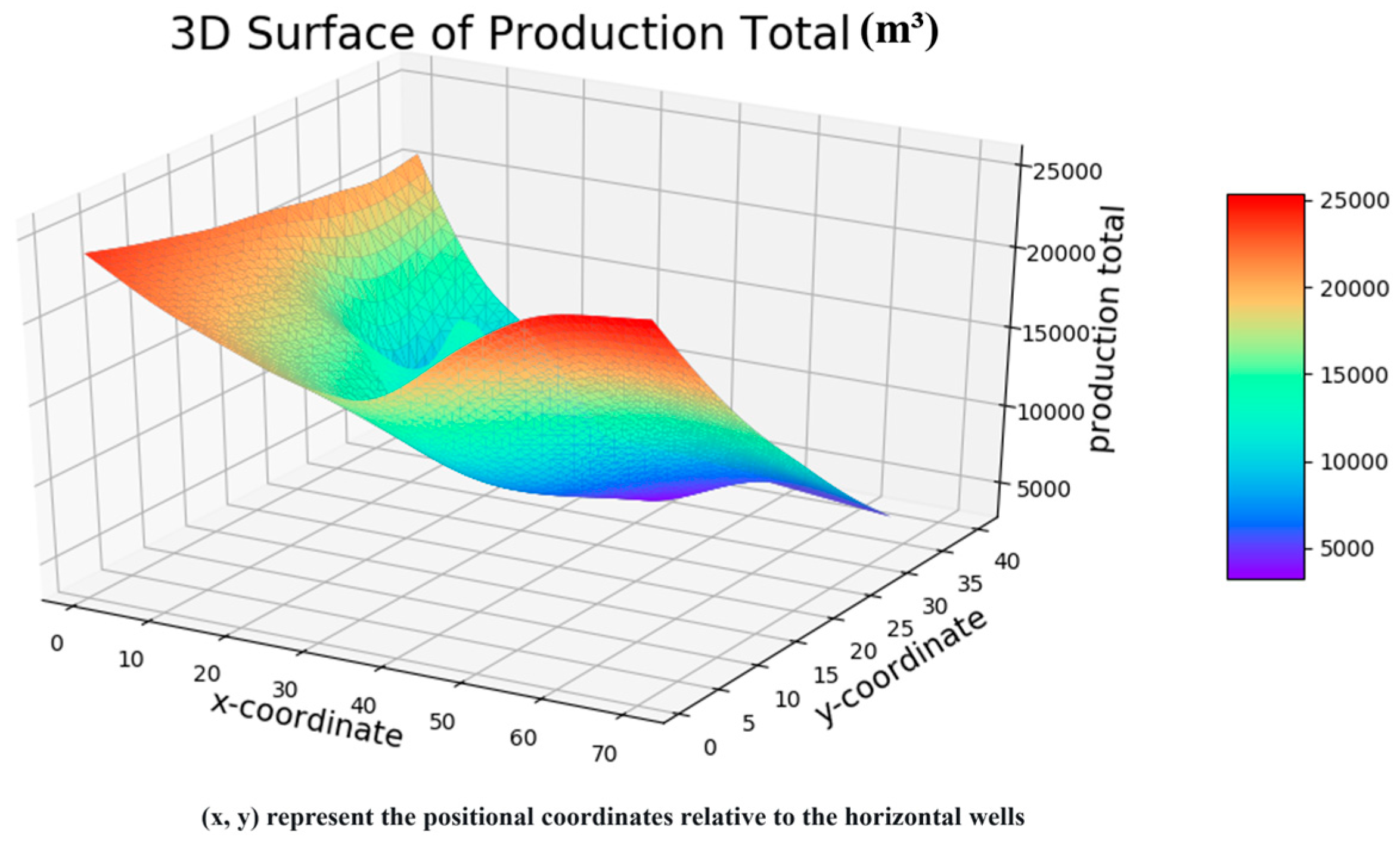
Figure 8.
3D visualization of the water cut (%) at the economic limit for different relative locations between vertical injection wells and horizontal production wells. The results highlight how well placement affects water breakthrough and sweep efficiency. The variables x and y represent the coordinate system relative to the horizontal well orientation.
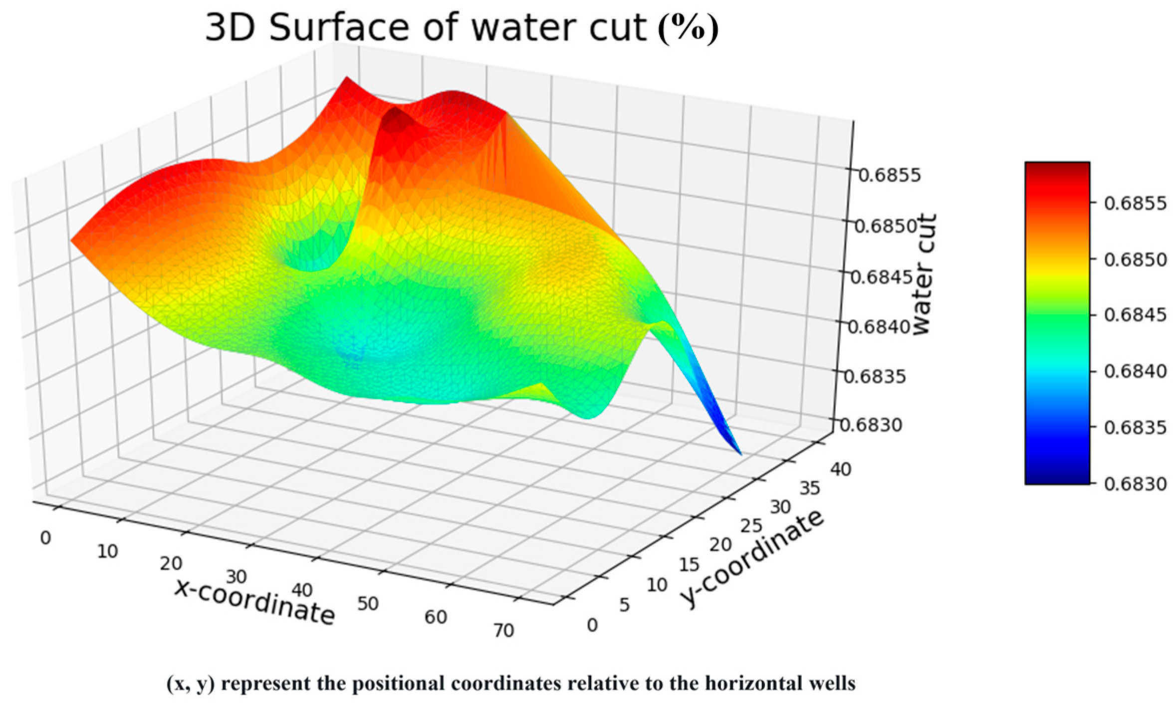
Figure 9.
Distribution of formation pressure at the end of depletion development.
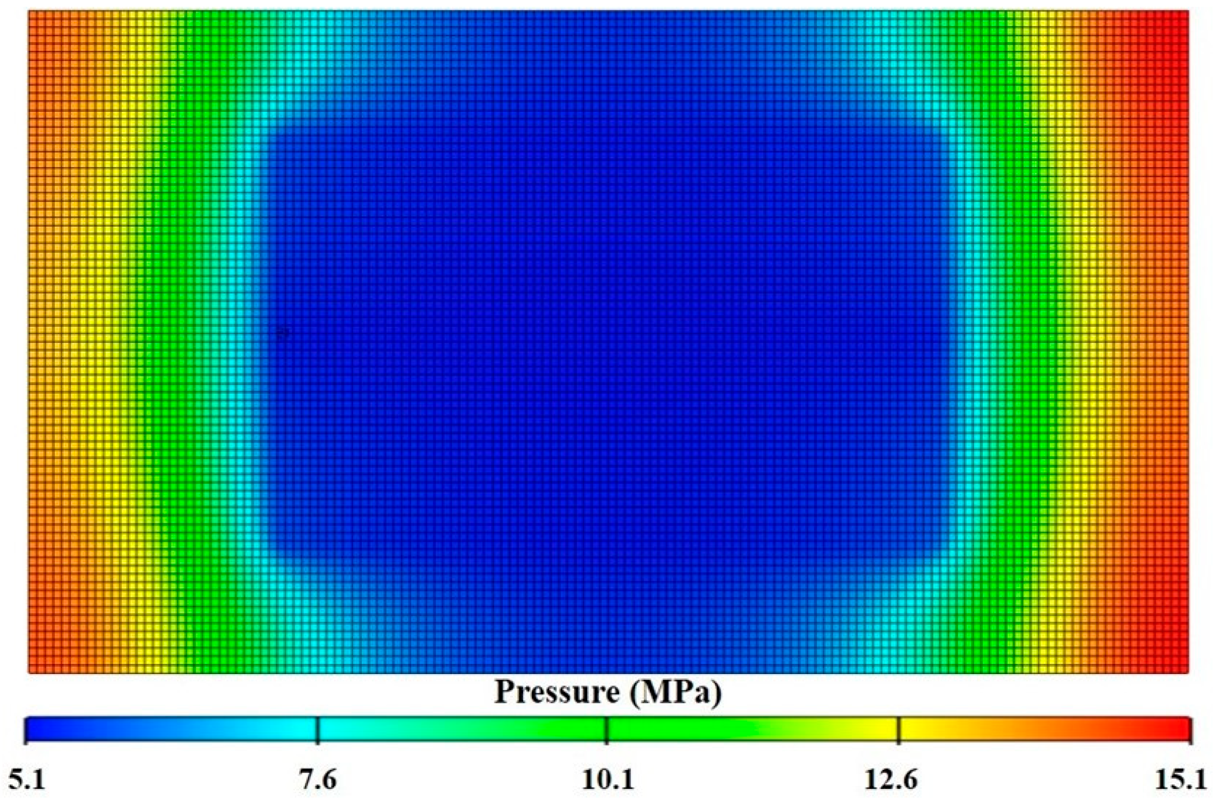
Figure 10.
The streamline distribution at the 1st day (a) and the end (b) of depletion development.
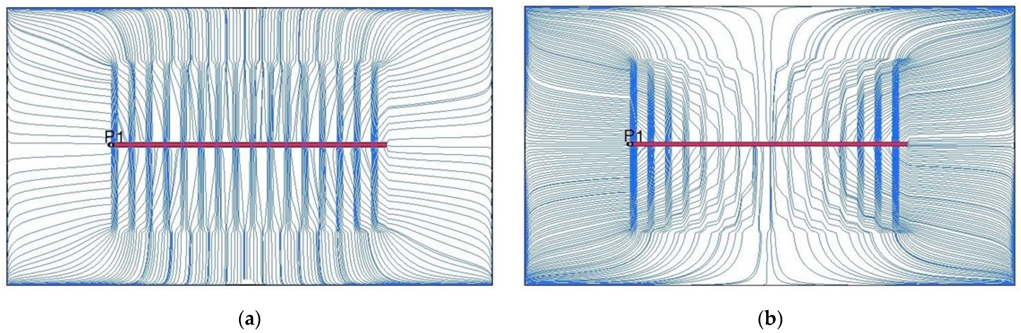
Figure 11.
Classification diagram of water injection regions.

Figure 12.
Irregular horizontal-vertical well group (3 vertical wells and 1 horizontal well).
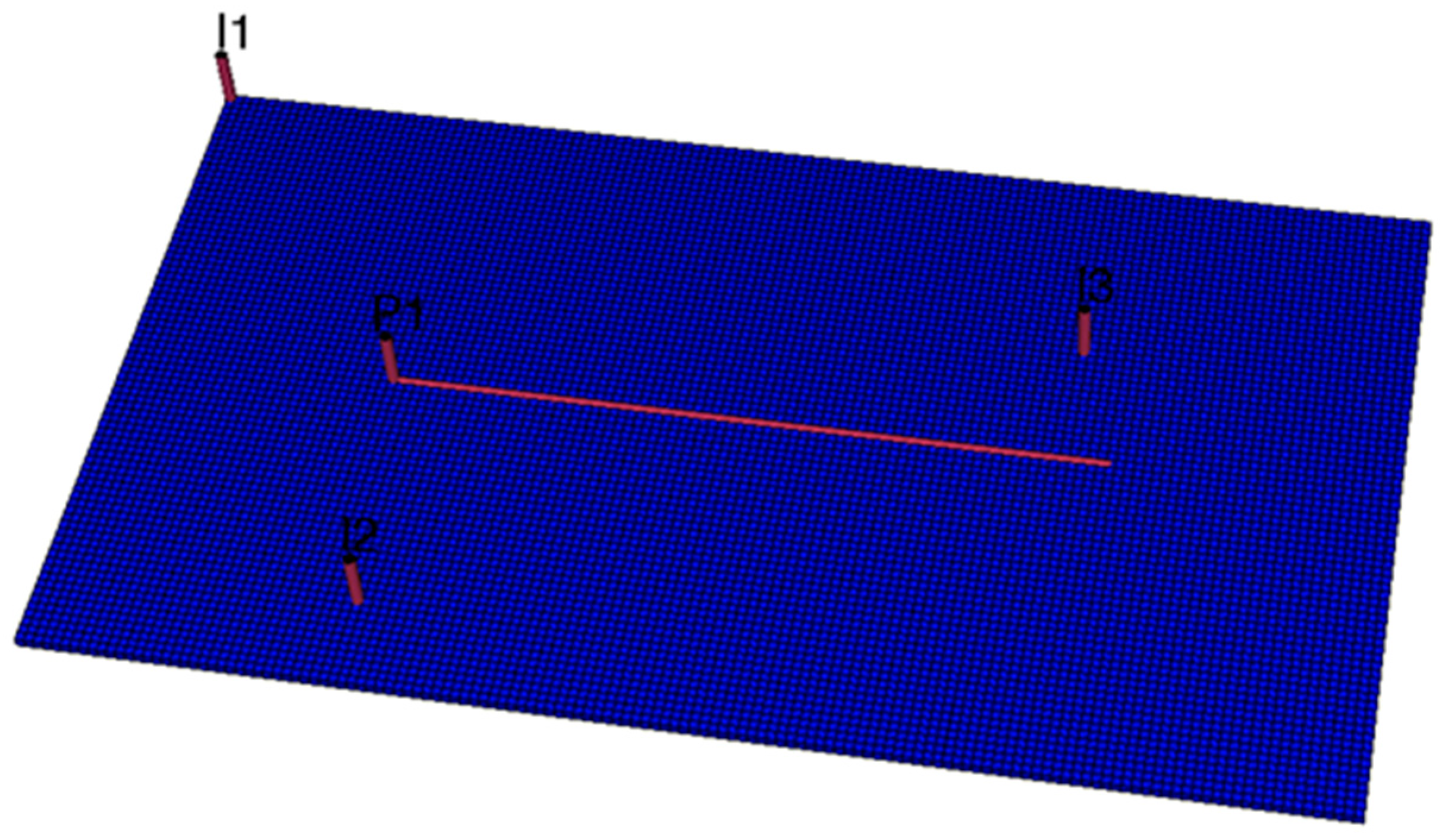
Figure 13.
Cumulative oil production.
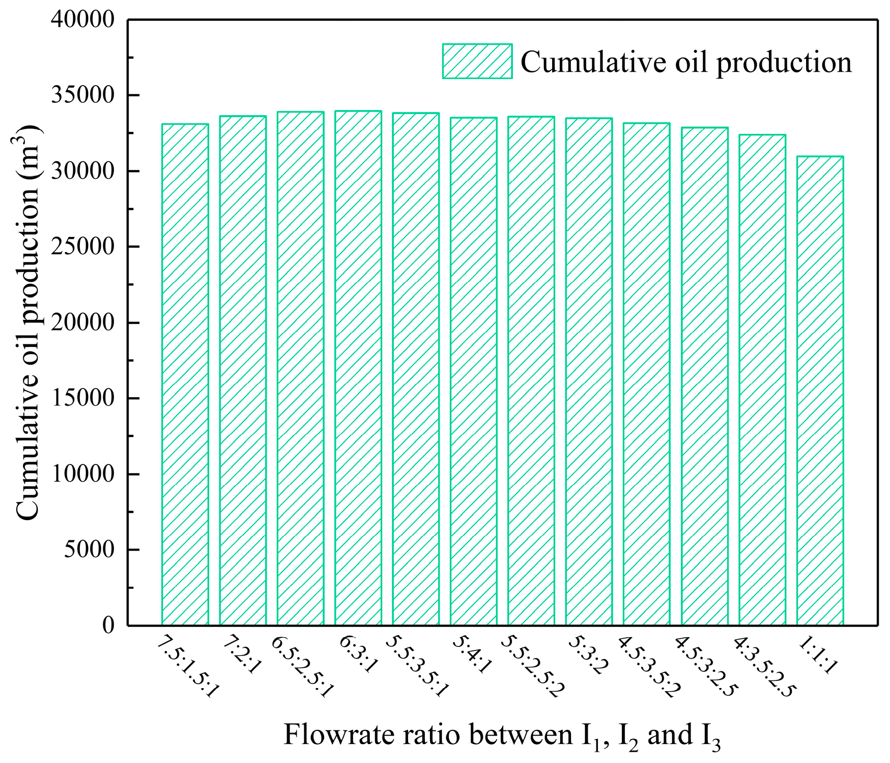
Figure 14.
Water cut.
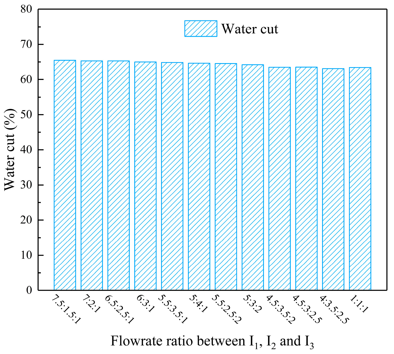
Figure 15.
Production rate.

Figure 16.
The streamline distribution of water flooding with different IRC (6100th days).
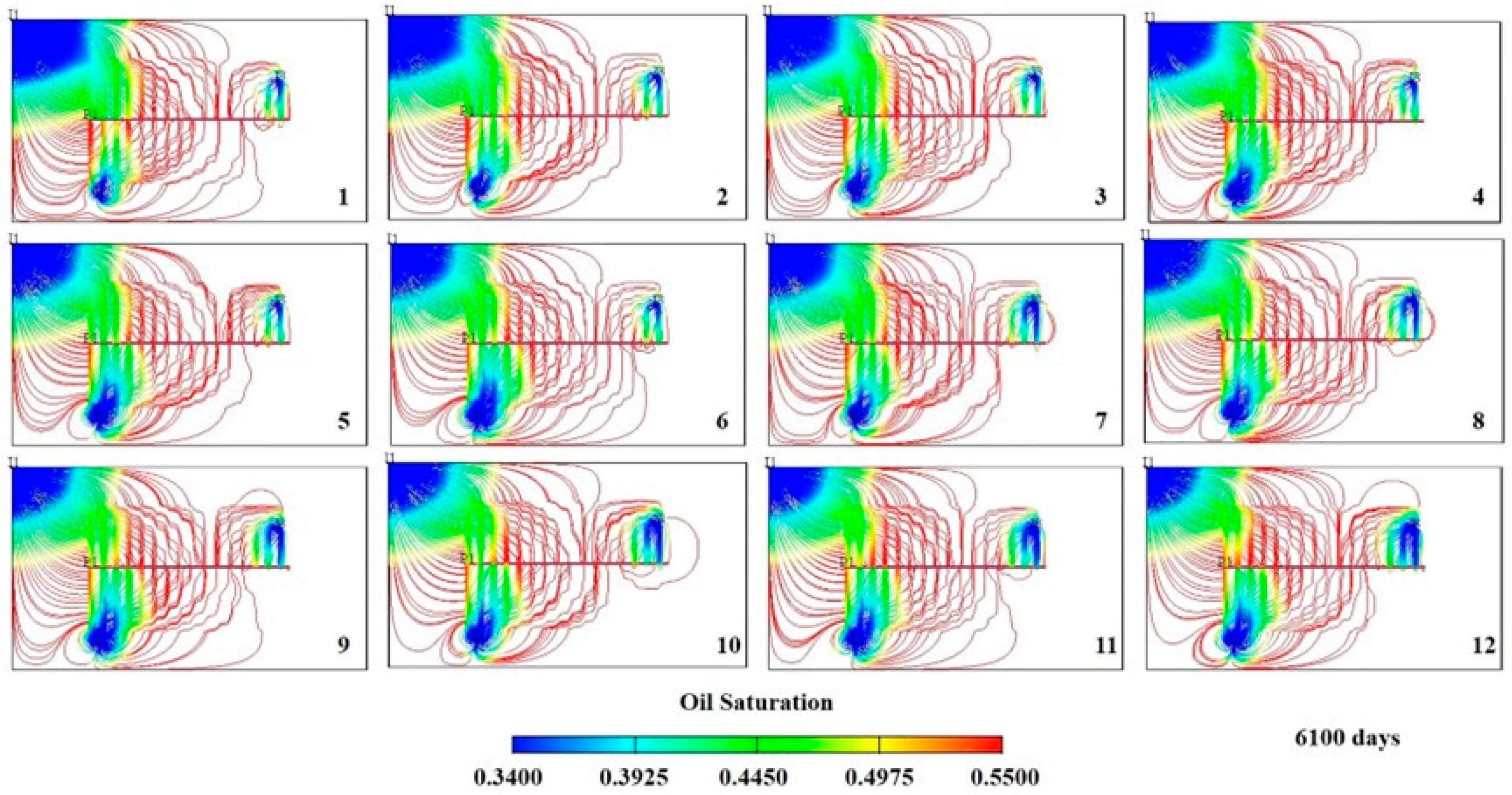
Figure 17.
The streamline distribution of water flooding with combination 1, 4 and 12 (2800th days and 4200th days respectively).
Figure 17.
The streamline distribution of water flooding with combination 1, 4 and 12 (2800th days and 4200th days respectively).
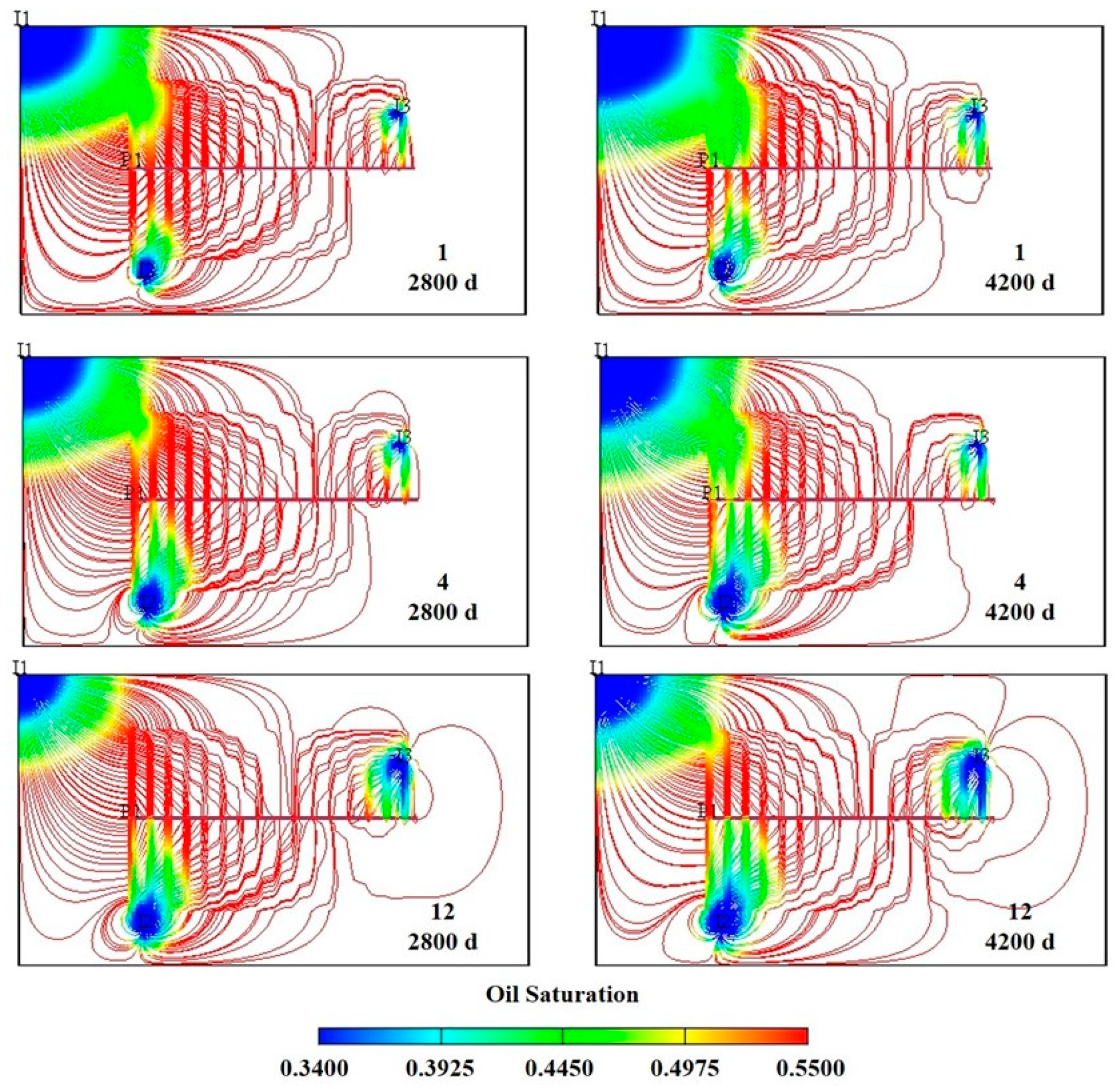

Table 1.
Key simulation parameters used in the model.
| Items | Values |
| The length of horizontal well/m | 800 |
| Average porosity | 0.15 |
| Average permeability of matrix region/mD | 0.23 |
| Average permeability of fracturing | 200 |
| region/mD | |
| Fracture width/cm | 20 |
| Fracture half-length/m | 250 |
Table 2.
Development Indicators When Production Declines to the Economic Limit Daily Oil Production.
Table 2.
Development Indicators When Production Declines to the Economic Limit Daily Oil Production.
| Model Number | Streamline Distribution | Production Duration (Days) | Cumulative Oil Production (m³) |
| 1 |  |
4430 | 24164 |
| 2 | 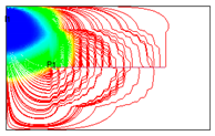 |
4160 | 22756.62 |
| 3 | 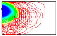 |
4080 | 21886.51 |
| 4 | 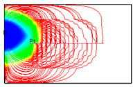 |
4050 | 21303.44 |
| 5 | 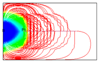 |
4090 | 21270.68 |
| 6 | 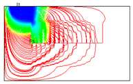 |
3800 | 20511.72 |
| 7 | 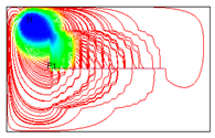 |
3110 | 17141.04 |
| 8 | 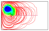 |
2590 | 14454.75 |
| 9 | 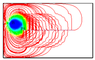 |
2130 | 11816.99 |
| 10 | 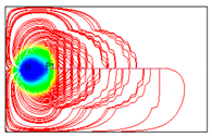 |
2000 | 10928.94 |
| 11 | 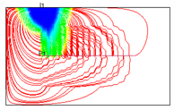 |
3390 | 18340.27 |
| 12 | 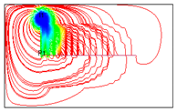 |
2220 | 12409.64 |
| 13 | 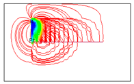 |
1180 | 7410.55 |
| 14 | 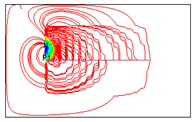 |
610 | 4646.06 |
| 15 | 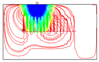 |
4420 | 23517.91 |
| 16 | 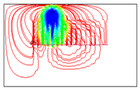 |
3170 | 17082.34 |
| 17 | 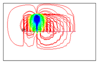 |
2030 | 11404.94 |
| 18 | 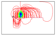 |
960 | 6185.23 |
| 19 | 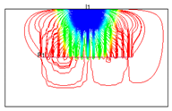 |
5040 | 26137.62 |
| 20 | 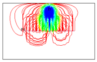 |
3410 | 18142.48 |
| 21 | 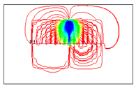 |
2130 | 11818.11 |
| 22 | 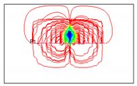 |
970 | 6232.69 |
Table 3.
Injection ratio coefficient (IRC).
| Number/# | IRC/R1 | IRC/R2 | IRC/R3 |
| 1 | 7.5 | 1.5 | 1 |
| 2 | 7 | 2 | 1 |
| 3 | 6.5 | 2.5 | 1 |
| 4 | 6 | 3 | 1 |
| 5 | 5.5 | 3.5 | 1 |
| 6 | 5 | 4 | 1 |
| 7 | 5.5 | 2.5 | 2 |
| 8 | 5 | 3 | 2 |
| 9 | 4.5 | 3.5 | 2 |
| 10 | 4.5 | 3 | 2.5 |
| 11 | 4 | 3.5 | 2.5 |
| 12 | 3.4 | 3.3 | 3.3 |
Disclaimer/Publisher’s Note: The statements, opinions and data contained in all publications are solely those of the individual author(s) and contributor(s) and not of MDPI and/or the editor(s). MDPI and/or the editor(s) disclaim responsibility for any injury to people or property resulting from any ideas, methods, instructions or products referred to in the content. |
© 2025 by the authors. Licensee MDPI, Basel, Switzerland. This article is an open access article distributed under the terms and conditions of the Creative Commons Attribution (CC BY) license (http://creativecommons.org/licenses/by/4.0/).
Copyright: This open access article is published under a Creative Commons CC BY 4.0 license, which permit the free download, distribution, and reuse, provided that the author and preprint are cited in any reuse.


