
Submitted:
01 April 2025
Posted:
02 April 2025
You are already at the latest version
Abstract
Let us consider the finite commutative ring R, whose unity is 1≠0. Its weakly zero-divisor graph, represented as WΓ(R), is a basic undirected graph with two distinct vertices, c1 and c2 that are adjacent if and only if there exist r∈ ann(c1) and s∈ ann(c2) that satisfy the condition rs=0. Let D(G) be the distance matrix and Tr(G) be the diagonal matrix of the vertex transmissions, in basic undirected connected graph G. The Dα matrix of graph G is defined as Dα(G)=αTr(G)+(1−α)D(G) for α∈[0,1]. This article find the Dα spectrum for the graph WΓ(Zn) for various value of n and also shows that WΓ(Zn) for n=ϑ1ϑ2ϑ3⋯ϑtη1d1η2d2⋯ηsds(di≥2,t≥1,s≥0) where ϑi’s and ηi’s are the distinct primes is Dα integral.
Keywords:
ring of integers modulo n
; weakly zero-divisor graph
; spectrum of graph
; Dα-matrix
1. Introduction
In this article, a commutative ring having identity shall be denoted by When an element , different from zero (0), exists such that , then the nonzero element is called a zero-divisor of R. is the collection of those zero-divisors in the ring R and .
The graph has been defined, where V denotes the set of vertices and E denotes the set of edges of G. When two distinct vertices of graph G, and are adjacent to each other in graph G, the notation represents this. In a graph G, the set of vertices adjacent to a vertex c is called its neighborhood; this neighborhood is represented by the notation . refers to the complete graph with m vertices. , the degree of vertex c, represents the number of edges incident with . If , then c is referred to as an isolated vertex. For every vertex , G is k-regular if . Let A be any square matrix and let be its different eigenvalues with multiplicities respectively. The of A is then denoted by (A), which is defined by
For a graph G, the matrix is a n-dimensional square matrix given by
The convex linear combinations of the adjacency matrix of G and the diagonal matrix of its vertices were proposed by Nikiforov [8]. This means that for where is referred to as the generalized adjacency matrix or matrix of G. Similarly, the generalized distance matrix was presented by Cui, He, and Tian [14] as the convex combination of and for where represents the distance matrix of G and the transmission matrix of G. If all the eigenvalues of a graph G are integers then G is said to be integral.
Nikmehre et al. [9] introduced the idea of a weakly zero-divisor graph of ring R. The weakly zero-divisor graph of ring R is represented by the symbol . There are two distinct vertices, and , that are adjacent if and only if there exists ann and ann, satisfying the condition . This undirected simple graph has a vertex set as the set of non-zero zero-divisors of R. The weakly zero-divisor graph’s spanning sub-graph is easily observed to be the zero-divisor graph of a ring.
The spectrum of the weakly zero-divisor graph of is found in this paper for various values of n. More information about spectrum of graphs and additional information on various types of graphs based on commutative ring can be found in [1,5,6,7,10,11,12]. The definitions, lemma’s and theorems that are utilized to support the main results are analyzed in section 2. eigenvalues of are looked into section 4, for where and are prime numbers with and are positive integers. Also, we calculate the spectrum of the weakly zero-divisor , for where ’s and ’s are distinct primes and shows that is integral.
2. Preliminaries
Definition 2.1.
“ Let be a graph of order m having vertex set and be disjoint graphs of order The graph formed the generalized join graph and whenever k and l are adjacent in G, joined each vertex of to every vertex of ."
indicates the number of positive divisors of a positive integer . For to not divide , we write . The greatest common divisor of and is shown by The number of positive integers smaller than or equal to that are relatively prime to is indicated by Eulur’s phi function . If , where are positive integers and are distinct primes, then is in .
Lemma 2.1
([4]). “If is a prime decomposition of , then
Let be the proper divisors of n. For consider the following sets
Moreover, observe that for , . As a result, the vertex set of has a partition formed by the sets . , as a result. The following lemma provides information about the cardinality of each .
Lemma 2.2
([15] [Lemma 2.1). ] “ Let be the proper divisor of n then for ”.
Lemma 2.3
([13]). Let n be represented as where are distinct primes and and . Then, consider the set of suitable divisors of n, denoted as . If then the induced sub-graph of by is
Corollary 2.1
([13]). Let be the proper divisor of positive integer The following assertions are true:
- (1)
- For , the induced subgraph of , formed by the vertices in the set is take two forms: either or .
- (2)
- For and , a vertex within is connected to either all or none of the vertices in in the graph
The sub-graphs created within the structure of can be classified as either complete graphs or empty graphs, as shown by the previously noted Corollary . The graph is created as a complete graph by utilizing the set of all suitable divisors of n, represented by the notation {}.
Lemma 2.4
([13]). are all the proper divisors of n.
The following theorem provides the generalized join graph’s spectrum in terms of the spectrum of adjacency matrix of regular graphs.
Theorem 2.2
([2]). Let H be a connected graph of order Let If, for , is a -regular graph of order then the spectrum of the H-join graphs is
where
Here and are distance from vertex i to j for
3. Methodology
Research in graph theory continues to flourish because it provides a link between discrete structures and pure as well as applied mathematics. Using sophisticated mathematical tools, the study’s method builds upon well-established ideas in algebra and graph theory to produce new results. Our efforts rely on using the content of existing research to expand on established findings and investigate fresh aspects of weakly zero-divisor graphs.
The analysis in this paper heavily relies on the use of matrix theory and linear algebra. In particular, spectral graph theory provides a strong framework for studying the interaction between algebraic and graph-theoretical characteristics. A crucial tool for capturing the structural features of the weakly zero-divisor graph of the ring
The primary objective of this study is to analyze the spectra of the weakly zero-divisor graph for a general class of n, where ’s and ’s are the distinct primes. To achieve this, we use the concept of new results on the - matrix of connected graphs, which was introduced by Diaz et al. [2].
4. Results
We will prove the main results of this paper in this section. For , the induced subgraph of , formed by the vertices in the set is either or Recall that the adjacency spectrum of complete graph and its complement graph on l vertices is given by
respectively.
Lemma 4.1.
Let n be the product of two different primes and . Then, the graph ’s spectrum is given by
The remaining two, eigenvalues of the graph are the roots of the characteristic polynomial
Proof.
The proper divisors of n are and and . Also, by the definition of Now by Lemma 2.4, we have . Therefore, by Lemma 2.2 and Corollary 2.1, we have and . Therefore, by Theorem 2.2, the spectrum of the graph is
and the root of characteristic polynomial of the matrix provided below, can be used to determine the remaining two eigenvalues
where . □
Theorem 4.1.
For distinct prime and , the spectrum of the is
where and the cardinality of the vertex set V of is given by The remaining six, eigenvalues of the graph are the eigenvalues of the matrix (3).
Proof.
Let , where , note that is complete graph on vertices . Now, by Lemma 2.4, we have,
Therefore, by Lemma 2.2 and Corollary 2.1, we have and .
The cardinality of the vertex set V of is given by Also we have and It follows that and for Therefore, by Theorem 2.2, the spectrum of the graph is
where And the matrix’s characteristic polynomial can be used to determine the remaining six eigenvalues,
where and □
Theorem 4.2.
Let where , is a prime and is a positive integer. Then, the spectrum of the graph consists of eigenvalue with multiplicity where The other remained , eigenvalues of the graph are eigenvalues of the matrix’s (4).
Proof.
For , where j is a positive integer and is a prime, the proper divisors of are By Lemma 2.4, we have
It follows that where is the cardinality of vertex set V of . Therefore, by Lemma 2.2 and Corollary 2.1, we get
Value of and for Therefore, by Theorem 2.2, the spectrum of the graph is consist of eigenvalue with multiplicity And the roots of the matrix’s (4) characteristic polynomial, can be used to determine the remained eigenvalues,
where and □
Theorem 4.3.
Let where , is a prime and is a positive integer. Then, spectrum of the graph consists of eigenvalue with multiplicity . The other remained , eigenvalues of the graph are eigenvalues of the matrix’s (5).
Proof.
Similarly as above Theorem 4.2, we can proof that the spectrum of the graph consists of eigenvalue with multiplicities , where is the cardinality of vertex set V of . The other remained , eigenvalues of the graph are eigenvalues of the matrix’s (5),
where , and □
If in Theorem 4.2, the resulting outcome gives the spectrum of .
Corollary 4.1.
The spectrum of for , consists of eigenvalue with multiplicity . The other remained 5, eigenvalues of the graph are eigenvalues of the matrix’s 6,
Where and
Theorem 4.4.
For distinct primes and , . The spectrum of the consists of eigenvalues,
The cardinality of the vertex set V of is given by and the roots of characteristic polynomial of the matrix (7) provides the remaining eigenvalues.
Proof.
Let , where , note that is complete graph on vertices . By lemma 2.4, we have
Therefore, by Lemma 2.2 and Corollary 2.1, we get
Consequently, the cardinality of the vertex set V of is given by and also and And it follows that and Therefore, by Theorem 2.2, the spectrum of the graph is
And the roots of the matrix’s (7) characteristic polynomial, can be used to determine the remaining eigenvalues
where and □
When we choose in Theorem 4.4, the conclusion can be derived.
Corollary 4.2.
For distinct primes and , the spectrum of the graph is given by
The cardinality of the vertex set V of is given by and the remaining four, eigenvalues of the graph are the eigenvalues of the matrix (8).
Proof.
Let , where , note that is complete graph on vertices By Lemma 2.4, we have =. Therefore, by Lemma 2.2 and Corollary 2.1, we have and .
The cardinality of the vertex set V of is given by and . It follows that, and Therefore, by Theorem 2.2, the spectrum of the graph is
And the matrix’s characteristic polynomial of matrix given in (8), can be used to determine the remaining four eigenvalues,
where and □
Example 4.1.
The spectrum of the weakly zero-divisor graph of is
The remaining four eigenvalues of the graph are the roots of characteristic polynomial of the matrix (9).
Figure 1.
Weakly zero-divisor graph .
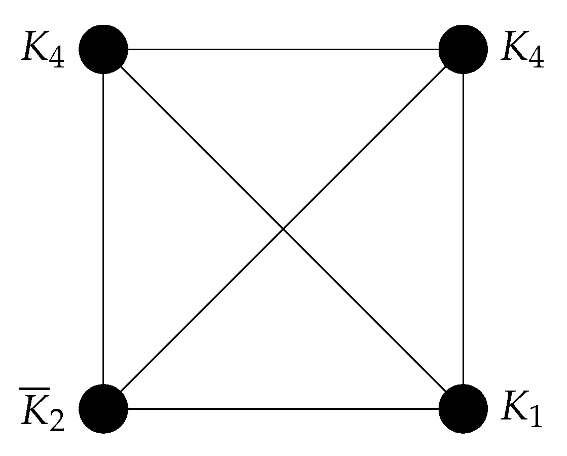
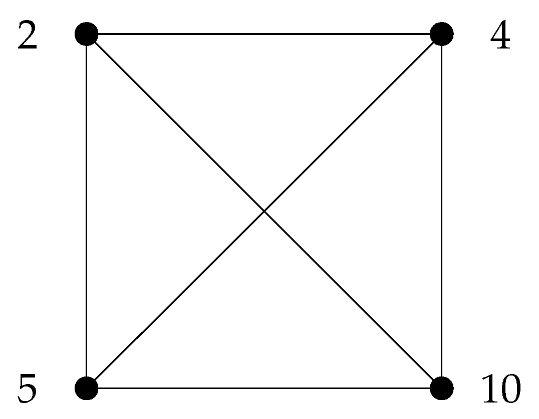
Figure 2.
Proper divisor graph .
From Corollary 4.2, the spectrum of the graph is given by
And the roots of characteristic polynomial of the matrix (9) provided below, are remaining four eigenvalues of the graph ,
where
Theorem 4.5.
Let where ’s and ’s are the distinct primes. Then, the spectrum of the consists of eigenvalues,
The cardinality of the vertex set V of the graph is given by, and the characteristic polynomial of the matrix (10) provides the other remained, eigenvalues. Also, if the eigenvalues of the matrix (10) are integers then the weakly zero divisor graph of for is integral.
Proof.
Suppose that where ’s and ’s are the distinct primes. Let Then, by Lemma 2.3, the following conclusions can be drawn: for each , we have and for we have The cardinality of the vertex set V of the graph is Also note that for , we have, for all and Therefore, by Theorem 2.2, the spectrum of the graph is
Note that all these eigenvalues are integers. And the roots of the matrix’s (10) characteristic polynomial, can be used to determine the remaining eigenvalues,
where and
If the eigenvalues of the matrix (10) are integers then the weakly zero divisor graph of for is integral. □
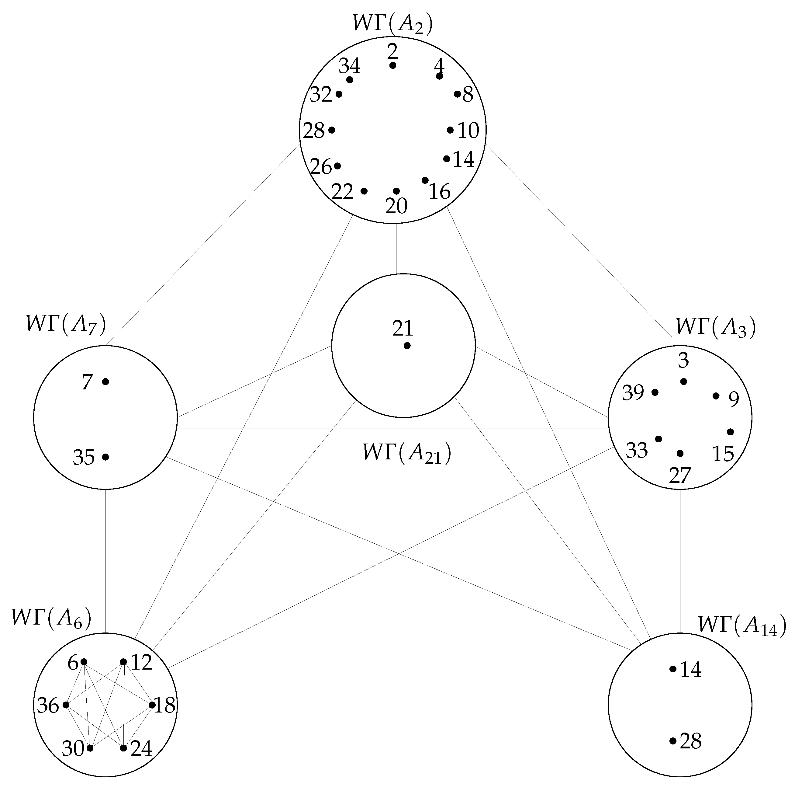
Example 4.2.
The spectrum of the weakly zero-divisor graph of shown in Figure 2., is
Other six remained, eigenvalues of the graph are the eigenvalues of the matrix (11).
The proper divisors of 42 are and Note that is complete graph on vertices and 21. Now by Lemma 2.4, we have . Therefore, by Lemma 2.2 and Corollary 2.1, we have and . The cardinality of the vertex set V of is 19. Now according the proper divisor sequence, we have, and further, we have and Consequently, the spectrum of the graph is given by Theorem 2.2.
And the matrix’s characteristic polynomial, can be used to determine the remaining six eigenvalues,
where
Figure 2.
Weakly zero-divisor graph .
5. Conclusion and Further Work
In this study, we have explored the spectrum of the weakly zero-divisor graph for a general class of n, where where ’s and ’s are the distinct primes. For this, we use the concept of new results on the - matrix of connected graphs, which was introduced by Diaz et al. [2]. We obtained the eigenvalues for several arrangements by using thorough calculations and basic algebraic properties of the weakly zero-divisor graph. This study shows how the algebraic structure of and the spectral features of its associated graph interact, building on earlier findings on particular classes of n.
The results show that the spectrum contains important information regarding the basic structure of weakly zero divisors. Specifically, the eigenvalue distributions and characteristic polynomials provide clarity on the modular arithmetic and divisors that underlie . The findings further support the significance of spectral graph theory in algebraic contexts by validating the existence of distinctive spectral patterns in specific classes of weakly zero-divisor graphs.
This study suggests various exciting paths for further exploration. One possible direction is to broaden the spectral analysis to encompass wider categories of finite commutative rings, with the goal of uncovering more profound connections between their algebraic characteristics and spectral parameters. An additional area worth exploring involves the investigation of further graph invariants, including the spectral radius, chromatic number, and connectivity, along with their relationships to the spectrum of weakly zero-divisor graphs. The spectra for higher powers of primes and rings with multiple prime factors could also be analyzed using sophisticated computer approaches, which could reveal complex patterns and features. Furthermore, it is necessary to conduct thorough research since the spectrum characteristics of weakly zero-divisor graphs may have useful implications in coding theory, cryptography, and error detection systems. It may be possible to identify significant similarities and differences between weakly zero-divisor graphs and other algebraically defined graphs, such as unit graphs or co-maximal graphs, by comparing their spectral properties.
Further one can calculate spectrum for co-zero divisor graph, unit graph, co-maximal graph and many more such graphs. This research not only deepens the theoretical insights into weakly zero-divisor graphs but also creates a strong basis for interdisciplinary studies that combine algebra, graph theory, and computational techniques.
Author Contributions
All authors made equal contribution.
Funding
The first author is supported by a project by Princess Nourah bint Abdulrahman University (PNU), Riyadh, Saudi Arabia, with Project No. PNURSP2025R231.
Conflicts of Interest
The authors declare no conflicts of interest.
References
- Anwar, M., Mozumder, M. R., Rashid, M., Raza, M.A. Somber Index and Somber spectrum of cozero-divisor graph of Zn. Results Math. 2024, 79(4), 146.
- Diaz, R. C., Pasten, G., Rojo, O. New results on the Dα- matrix of connected graphs. Linear Algebra Appl. 2019, 577, 168–185. [CrossRef]
- Diaz, R. C., Pasten, G., Rojo, O. On the minimal spectral radius of graphs subject to fixed connectivity. Linear Algebra Appl. 2020, 584, 353–370. [CrossRef]
- Koshy, T. Elementary number theory with application, 2nd ed., academic press: cambridge, UK, 1985.
- Lin, H., Liu, X., Xue, J. Graphs determined by Aα-spectra. Discrete Math. 2019, 342, 441–450. [CrossRef]
- Lin, H., Xue, J., Shu, J. On the Dα-spectral radius of graphs. Linear Multilinear Algebra 2019, 62, 1563–5139.
- Mozumder, M. R., Rashid, M., Khan, A. I. A. Exploring Aα spectrum of the weakly zero-divisor graph of the ring Zn. Discrete Math. Algorit. Appl. 2025. [CrossRef]
- Nikiforov, V. Merging the A-and Q-spectral theories. Appl. Anal. Discrete Math. 2017, 12, 81–107. [Google Scholar] [CrossRef]
- Nikmehr, M. J., Azadi, A., Nikandish, R. The weakly zero-divisor graph of a commutative ring. Rev.Union Mat.Argent. 2021, 35, 105–116.
- Rashid, M., Alali, A. S., Mozumder, M. R., Ahmed, W. Spectrum of the cozero-divisor graph associated to ring Zn. Axioms 2023, 12, 957. [CrossRef]
- Rashid, M., Mozumder, M. R., Anwar, M. Signless Laplacian spectrum of the cozero-divisor graph of the commutative ring Zn. Georgian Math. J. 2024, 31(4), 687–699.
- Rashid, M., Mozumder, M. R., Ahmed, W. On signless Laplacian eigenvalues of Zn. Palestine Journal of Mathematics 2024, 13(4), 955–961.
- Shariq, M., Mathil, P., Kumar, J. Laplacian spectrum of weakly zero-divisor graph of the ring Zn. arXiv2023,arXiv:2307.12757.
- SY. Cui, JX. He, GX. Tian. The generalized distance matrix. Linear Algebra Appl. 2019, 563, 1–23. [CrossRef]
- Young, M. Adjacency matrices of zero-divisor graphs of integer modulo n. Involve 2015, 8, 753–761. [Google Scholar] [CrossRef]
Disclaimer/Publisher’s Note: The statements, opinions and data contained in all publications are solely those of the individual author(s) and contributor(s) and not of MDPI and/or the editor(s). MDPI and/or the editor(s) disclaim responsibility for any injury to people or property resulting from any ideas, methods, instructions or products referred to in the content. |
© 2025 by the authors. Licensee MDPI, Basel, Switzerland. This article is an open access article distributed under the terms and conditions of the Creative Commons Attribution (CC BY) license (http://creativecommons.org/licenses/by/4.0/).
Copyright: This open access article is published under a Creative Commons CC BY 4.0 license, which permit the free download, distribution, and reuse, provided that the author and preprint are cited in any reuse.


