
Submitted:
28 January 2025
Posted:
29 January 2025
You are already at the latest version
Abstract
In the framework of the Robertson–Walker metric, we investigate the behavior of a subordinated cosmic scale factor a(t). The parent process a˜(τ) is modeled as a sharp phase transition between two Einstein universes, each with different total energies E1 and E2, at a specific moment τc of the operational time τ. To account for the effect of random clocks, which may arise from differences in the physical properties of dark matter and ordinary matter, this model incorporates a random operational time in the form of an inverse, strictly increasing Lévy-type subordinator. As an observable in physical time t, a(t) is defined as the mean of the parent process over an ensemble of realizations of the inverse subordinator. Specifically, we show that, under certain parameter regimes, the evolution of a(t) mimics primordial inflation, subsequent decelerated expansion, and cosmic acceleration. Employing energy conservation in a closed, expanding universe, we discuss the possibility of incorporating matter density evolution. Furthermore, we establish the emergence of dark energy. We believe that this work introduces a novel application of fractional calculus to cosmology.
Keywords:
Inverse subordinator
; L'evy-type subordinator
; Einstein Universe
; Dark energy
; Cosmological inflation
; Accelerating Universe
1. Introduction
The current standard cosmological model, the -cold dark matter (CDM) model, has been successful in explaining both the homogeneous expansion of the Universe and the 2.7 K cosmic microwave background (CMB) radiation [1]. Although CDM provides a remarkable fit to most available cosmological data, it lacks the deeper underpinnings necessary to connect with fundamental physical laws. In particular, the physical evidence for inflation, dark matter (DM), and dark energy (DE) so far arises only from cosmological and astrophysical observations [2]. Moreover, as measurements become increasingly precise, discrepancies among key cosmological parameters have emerged. For example, Planck measurements of the CMB at redshift yield a CDM-based value for the present-day Hubble constant of [3,4]. In contrast, several late-time, model-independent measurements of distances and redshifts give [5]. Furthermore, recent observations by the James Webb Space Telescope (JWST) indicate that the structure and masses of very early galaxies at high redshift are in strong tension with the CDM model, given that the Universe’s age of about 13.8 Gyr leaves insufficient time for the formation of massive galaxies at high redshifts [6]. In addition, the tension of the curvature parameter is measured between the Planck 2018, CMB lensing, and baryon acoustic oscillation (BAO) data [4]. Especially, Planck 2018 CMB data alone indicate a strong preference for closed universes over open ones [4,7]. This result contrasts with other data sets such as Planck CMB lensing or BAO which suggest a flat universe. However, in the modern era there is a strong research community bias toward a flat universe. It should be noted that very few conclusions about the kinematics and dynamics of the universe have been drawn without relying on model assumptions, typically those of the CDM model. In this predicament, it is crucial not to adhere too tightly to the standard model [2]. Consequently, the precise measurements from various astronomical missions have led to a striking tension in cosmological parameters, underscoring the strong need for alternative cosmologies to the canonical CDM paradigm.
In recent decades, the application of fractional calculus in a wide range of fields—such as biology [8], quantum mechanics [9], and neuroscience [10,11]—has grown rapidly. Moreover, experimental evidence shows that anomalous diffusion, characterized by a mean-square displacement of particles , is ubiquitous in nature, indicating that slow transport may be generic for complex heterogeneous systems [12]. This type of dynamics is generally understood to arise from two distinct mechanisms [13]. The first mechanism is formulated within the framework of the generalized Langevin equation, which incorporates a slowly relaxing memory-friction term [14,15,16,17]. The second mechanism is based on the concept of continuous-time random walks (CTRW) [18,19], wherein the time dependence of the random walk is governed by a slowly decaying waiting-time distribution for , reflecting the presence of deep traps in the system [20]. A convenient description of the continuous realization of the CTRW scheme—via a random operational time known as the subordination procedure—was proposed in [21]. Comprehensive treatments of the subordinated process within the CTRW framework, along with discussions on how these approaches can be generalized for different diffusive scenarios in complex systems, are given in [22,23,24,25,26,27].
In the present paper, inspired by the Bohr model of the atom, in which electron orbitals correspond to stationary energy levels, we consider the primordial Universe as undergoing a sharp (vacuum-phase) transition at a specific internal (operational) time between two Einstein Universes. Each of these Universes is characterized by a distinct stationary energy level with scale factors: for , and for . Additionally, we assume that the ticks of the internal clock are accumulated from two independent channels of activity: one corresponding to ordinary matter and the other to dark matter. This sharp transition, described above, is treated as the parent process evolving in internal time.
To determine the scale factor of the Robertson–Walker (RW) metric,
at the observable (physical) time t, we introduce an inverse Lévy-type subordinator to relate the internal and physical times. Here, c is the speed of light, r, , and are spherical coordinates, and determines the geometry of the space. We then assume that the scale factor can be obtained as the mean of over an ensemble of realizations of the inverse subordinator, i.e.,
The main contribution of this paper is as follows. Within the framework of the proposed subordinated model, we provide exact analytical formulas for the dependence of the scale factor on observable time. Based on these expressions, we find that the kinematics of in physical time qualitatively mimic the well-known expansion history of the Universe through three distinct eras: inflation, decelerated expansion, and cosmic acceleration. Moreover, by invoking energy conservation, we attempt to phenomenologically include the effects of the subordinated process by describing the evolution of the matter density in the model. It is shown that this approach predicts the emergence of a time-dependent dark energy, which vanishes as . In this scenario, the accelerated expansion of the Universe eventually ceases, leading to a new period of decelerated expansion; the Universe then continues to grow forever at an ever-decreasing rate.
The structure of the paper is as follows. In Section 2, we present the proposed model. In Section 3, we derive asymptotic formulas for the scale factor . In Section 4, we discuss the behavior of and illustrate its characteristic features. Section 5 addresses the inclusion of matter-energy in the model, deriving formulas for the evolution of the matter and dark energy densities. Section 6 offers brief concluding remarks. Finally, additional formulas are provided in the Appendixes.
2. The Model
For the reader’s convenience, we briefly summarize the main features of the subordination method in subsection 2.1, adapted from Ref. [11].
2.1. Subordination Procedure
The formulation of the subordination scheme is based on a system of coupled Langevin equations [10,21,22],
where is a time-independent function, and the trajectories of the random walk are parameterized by the variable . The Markovian noises and are assumed to be independent. In the context of the CTRW scheme, must be positive due to causality. Here and in the following, stochastic variables are denoted with capital letters (e.g., T), and possible values of these variables with the corresponding lowercase letters (e.g., t). The system (2) can be interpreted as a standard Langevin equation in an internal time that is subjected to a random time change described by the second equation. The internal time plays the role of the number of jumps (clock ticks) performed along the trajectory and is successively delayed by trapping events. The physical time t is modeled by an independent process , known as the subordinator. It is the sum of independent, identically distributed random waiting time intervals between the jumps. The subordinator is defined as a strictly increasing Lévy motion with the characteristic function
where is the probability density function (PDF) of , and is called the Lévy exponent [25]. If is a Bernstein function, then the subordinator is well-defined: it starts from zero and is a pure-jump process with strictly increasing sample paths [25]. To complete the subordination procedure, an inverse subordinator is introduced, which measures the evolution of the internal (operational) time as a stochastic function on physical time t and fulfills the following first passage time relation:
The PDF of is given by
If the Lévy exponent is a Bernstein function, then the inverse subordinator , which has nondecreasing continuous trajectories, can be used as a time arrow [25]. The process of primary interest, i.e., the random walk motion as seen by the observer in physical time t, is now obtained as a combined random function . The process is called a parent process, and the resulting process is subordinated to the parent process (referred to as the subordinated process).
2.2. Einstein Universe
The key equations of spatially homogeneous and isotropic cosmology are the Friedman equations, which are the field equations of general relativity applied to the RW metric (1):
where an overdot denotes a time derivative, is the total energy density of the Universe (sum of ordinary matter, radiation, dark matter), p is the total pressure (sum of pressures from each component i), and and G are the cosmological and gravitational constants, respectively [1]. As the metric (1) requires the stress-energy to take the perfect fluid form, the evolution of the energy density is governed by the ratio of pressure to energy density for each component i:
Hereafter, without a subscript refers to
Under physically reasonable assumptions
a static solution of equations (6)-(9) is possible only if i.e., the Universe is closed with a finite volume . The corresponding solution, called the Einstein Universe, is characterized by two free parameters (a and ) as follows:
Eventually, the total energy E of the Universe is given by
However, it should be noted that the Einstein Universe is unstable against expansion or contraction.
2.3. Kinematic Model for the Scale Factor
2.3.1. Fundamentals
The main assumptions of the model are as follows:
- 1.
- Drawing an analogy with the Bohr model of the atom, we assume that the primordial Universe, in internal time , can only exist in sharply defined stationary states with unique energies, which are described by Einstein Universes. The ability for transitions between these states is also postulated.
- 2.
- The internal and physical times are interconnected via a Lévy-type subordinator. It is hypothesized that the corresponding Lévy exponent accounts for the aggregation of ticks from two independent clocks, representing ordinary matter and dark matter.
- 3.
- The observable scale factor in physical time t is conceptualized as the mean outcome of a scale factor jump between two stationary states of the primordial Universe, averaged over an ensemble of realizations of the inverse subordinator.
2.3.2. Subordinated Scale Factor
The parent process is modeled as a jump process:
where . Here, represents the scale factor of an Einstein Universe, and is the critical time at which the transition between these states occurs. According to Hypothesis 3 from Subsection 2.3.1, the observable scale factor can be expressed as:
This formulation uses the relationship defined in equation (5). Consequently, the expansion rate is given by:
indicating that it is proportional to the (PDF) of the subordinator . Completing the model description requires specifying the structure of the Lévy exponent , a critical component of the model. Typically, for subdiffusion phenomena, the Lévy exponent is given as:
where , a constant, has the dimension of time, is the gamma function, and is known as the memory exponent [27]. In this particular case, following from Equations (3) and (5), the mean number of ticks of the internal clock within the time interval is:
and the corresponding PDF of is:
where is the one-sided -stable PDF [30].
As demonstrated by Ref. [30], one-sided laws can be transformed into non-oscillating integrals, which are more convenient for numerical calculations:
where
To determine the Lévy exponent in our model, we consider baryon matter and dark matter as two independent escape (clock ticks) channels acting in parallel. It is assumed that for both channels, their contributions to the number of ticks of the internal clock are determined by Eq. (17), with different memory exponents: for dark matter and for baryon matter. The total mean number of escape events (ticks) of the internal clock within the time interval can be expressed as:
where the non-negative coefficient characterizes the relative weight of the dark matter compared to the total matter (baryon matter plus dark matter). From Eqs. (3) and (5), it follows that the Lévy exponent is related to the Laplace transform of the mean value through:
Thus, the appropriate Lévy exponent can be expressed as:
Equation (23) along with Eq. (3) completes the subordinated model for the scale factor , as considered in this paper. Finally, we note that properties of the with similar structure have been considered in [23] and [25], where it is shown that such a Lévy exponent is a Bernstein function (see also Appendix A).
3. Asymptotic Behavior of the Scale Factor
Hereafter, we assume that the memory exponent for DM is much smaller than the memory exponent for the baryon matter, i.e.,
In this context, it is important to note that in the specific case where and , the PDF of the subordinator reduces to a -function:
i.e., in the case of ideally homogeneous baryon matter distribution (without DM), the physical time and the operational time coincide. A slight deviation of from 1, in inequality (24) is assumed to model the heterogeneity of the baryon matter, such as the time dilation effects observed at black holes, neutron stars, etc.
3.1. The Short-Time Limit
From Eqs. (21) and (24), it follows that in the short-time limit, (or ), the smaller memory exponent, , dominates. Thus, the limiting behavior of for is related to the one-sided Lévy -stable PDF as follows (see Eqs. (18)-(20)):
Referring to the behavior of the function , as discussed in Refs. [30] and [31], we conclude that is monomodal. As t increases, increases exponentially from zero to a maximum, then decreases monotonically. If z is sufficiently small (), i.e.,
the position, , of the maximum of is given by (see Appendix B):
and
In this case, the PDF of the subordinator is given by
The cumulative probability of the subordinator can be expressed as
where
Here, we emphasize that the formulas (28)-(32) are applicable only within a finite time interval, determined by the condition and Eq. (27). Eqs. (28)-(32) are particularly suitable for analyzing the behavior of the scale factor and the expansion rate at small time values, e.g., for describing the inflation era of the Universe. Notably, from Eqs. (28) and (29), it is observed that the peak of becomes more pronounced and its position rapidly shifts towards shorter times as the memory exponent decreases.
3.2. The Long-Time Limit
In the long-time limit, where (or ), the larger memory exponent in Eq. (21) dominates. The limiting behavior of , as encoded in expression (23), yields the asymptotic form:
Thus, in this asymptotic limit, only the baryon matter contributes, causing to tend to zero like .
Numerical investigations of the inverse Laplace transform of Eq. (3) with the Lévy exponent (23) indicate that under condition (24), a bimodal dependence of on t may be generic, especially if . Although we are not able to derive a simple estimator for the position of the second peak, , of at moderate time values, it seems that in the particular case given by Eq. (24), is approximately determined by:
4. A Numerical Illustration of Kinematic of the Scale Factor
In the case of the Lévy exponent (23) a convinient formula for the calculation of can be obtained if , [10,11]. In this case the appropriate contour in complex plane for the evaluation of the inverse Laplace transform of can be transformed to the Hankel contour with a cut along the real negative semiaxis (in the half-plane the poles are absent). Thus, the PDF of the subordinator is given by
Three of the most important parameters of the Universe described with the metric (1) are the values of the Hubble parameter
and the deceleration parameter
in the present epoch (i.e., and ), and the redshift of photons (with wavelengths ) emitted from a distant source at time t
Here and below, a subscript “0” on a parameter denotes its value at the present. Our model for expansion of the Universe is described by 7 parameters: , , , , and . To illustrate a possible evolution of the scale factor in physical time, Eqs. (14) and (15), we specify these parameters as follows:
The parameter value (Planck-length) is partly inspired by the paper [32], where the Universe was modeled as a closed RW spacetime which starts with inflation from a nonsingular state characterized by the Planck density and the Planck radius . The parameter value , which characterizes the relative weight of the dark matter in comparison with total matter, corresponds to the observed rotation velocities of stars in galaxies, and is also required to give an account of cosmological structure formation and gravitational lensing, [1]. As mentioned in the Section 3, a slight deviation of the memory exponent from 1 is assumed to model heterogeneity of the baryon matter. The maximum radius of the Universe is a free parameter, which must be large enough to guarantee the observed fact that the Universe is nearly spatially flat [1]. The remaining parameters , , and are chosen so that duration of the inflation era is comparable with s, Eq. (28), and that the well established today’s values of and the age of the Universe , , in the epoch of last scattering, when photons and baryons decoupled, are in accordance with results computed from Eqs. (36) and (38), respectively.
Table 1 presents cosmological parameters computed from Eqs. (14), (23), and (35)-(39) for our model (OM), comparing them with the consensus CDM model and the hybrid tired light model with covarying coupling constants (CCC+TL) [6].
It is remarkable that our model predicts the age of the Universe at Gyr, compared to the generally accepted value of 13.8 Gyr. This significant difference also extends to values and when compared to those predicted by the CDM model. Although such discrepancies may raise concerns, they potentially resolve the “impossible early galaxy” problem identified by recent JWST observations. These observations confirm the existence of galaxies at high redshifts that, according to the CDM model, would have existed only about 0.3 Gyr after the Big Bang—much sooner than expected from traditional galaxy formation models [6]. Notably, the CCC+TL model [6] was developed specifically to address this issue. As evident from Table 1, both our model and the CCC+TL model predict a sufficient extension of cosmic time to allow for the formation of large galaxies at these high redshifts.
Figure 1 illustrates how the expansion rate evolves over time under the parameters specified by Eq. (39). Notably, exhibits a bimodal form, indicating significant dynamic changes in the Universe’s expansion rate at different epochs. It is seen that the evolution of the expansion rate is characterized by the following scenarios: by increasing time it starts from zero at and increases very rapidly to the maximum value cm/s at s. In this time interval the scale factor a, see Eqs. (14) and (31), increases from the Planck length ( cm) to the macroscopic value cm displaying so the inflation era of the Universe. For further increasing values of t the expansion rate decreases monotonously to a minimum cm/s at Gyr . After that the expansion of the Universe is accelerating up to the time Gyr at which the second maximum of the function appears, . At larger times, , is again monotonically decreasing , and tends to zero at , .
5. Matter and Radiation in the Universe
In the proposed model, we utilize the concept of a sharp transition at an internal time from one Einstein Universe (EU1) with total energy to another (EU2) with total energy . This approach builds on the notion that the evolution of energy in the internal time can be modeled as a jump process:
Accordingly, in physical time, the total energy evolves as follows:
Given that the scale factor is significantly larger than (Planck length), it is reasonable to assume that the dominant contributions to the energy in are from dust matter (cold dark matter plus non-relativistic baryon matter) and isotropic radiation, with pressures and (where is the radiation energy density), respectively. From Eqs. (8), (9), and (12), we derive:
where is the Planck energy and represents the total energy of radiation and relativistic particles in , with .
To proceed further, it is reasonable divide the energy density into three parts
where , , and correspond to dust-matter, radiation, and DE, respectively. Using the energy conservation for each component separately
the expanding Universe analogue of the first law of thermodynamics , one can write
In addition to these equations we define two parameters
which can be estimated via observations. In the consensus cosmological model presented in [1] the current values of these parameters are given by and . With the help of Eqs. (14) and (41)-(46), it is possible to express the energy densities and the state-parameter as (see also Appendix C)
and
Let us take, to be specific, the parameter values from Eq. (39); in this case . In the case of large time, , the contribution of the EU2 to is dominant
and the density of the DE tends to zero, , indicating that the DE is generated by a contribution of the primordial EU1 to . For limiting values of the energy densities and we obtain
Thus in this epoch the dust-matter (cold DM + nonrelativistic baryon matter) dominates. It is notable that corresponding value of the cosmological constant in the Einstein Universe is very small (see also Eq. (11)).
We will now consider the behavior of the energy at short-time limit, , where the contribution of the primordial Einstein Universe (with ) to dominates. In the parameter regime described by Eq. (39), from Eq. (49) we get
so that in this Einstein Universe the universe matter had an equation of state
which is usually assumed by inflation models (see, e.g., [1] and [32]). Because this, in the very early period of the Universe, the matter behaved very differently from the matter we know. In the short-time limit, , from Eqs. (11), (12), (41), and (53) it follows that
with and
It is somewhat surprising that the described model predicts a transition from a higher energy level to a lower one , with . At first glance, Eq. (12) seems to suggest that energy E increases as the scale factor a increases. However, this conclusion is misleading because it does not consider potential changes in the equations of state. The estimated value of greatly exceeds the Planck density . This suggests that the classical description may not hold for such extreme densities, indicating the need for a quantum gravity theory—which remains undeveloped—to unify gravity with other fundamental interactions as suggested by [1].
Given this situation, we consider two possibilities. The first is that the model proposed here may only be applicable after a certain time, seconds, where . It is remarkable that the time interval is much shorter as the Planck time s. The second possibility involves interpreting the cosmological constant in Eqs. (6) and (7) as a representation of vacuum energy, with an energy density given by:
where the vacuum pressure . Consequently, the total energy density of an Einstein Universe can be expressed as:
It should be noted that the value of , corresponding to the very large magnitude of the cosmological constant from Eq. (56), aligns with some estimates from quantum field theory for the energy density associated with the quantum vacuum. Within the CDM model, such a significant quantum vacuum energy density presents a well-known issue—referred to as the cosmological constant problem—where the quantum vacuum energy density exceeds the density predicted by the CDM model by approximately 120 orders of magnitude [1].
In our proposed model, the total energy density , corresponding to , is on the order of the Planck density:
and the total energy of EU1 is given by:
To an observer, the universe appears to begin expanding at time from a state characterized by the Planck scale factor , the Planck energy density , and the total mass of the universe being the Planck mass (approximately g). It remains an open question whether our model can shed light on the vacuum-energy problem in cosmology.
Finally, our analysis is restricted to a single transition between two stationary states of the parent process (refer to Eq.(13)). Here, the model predicts that the accelerated expansion of the universe eventually ceases, followed by perpetual expansion at an ever-decreasing rate. Our findings serve as a promising foundation for exploring more elaborate models. For example, the model could be extended to include an inverse transition from EU2 back to EU1 at a specific internal time . According to this version, the universe would reach a maximum radius before contracting back to EU1, allowing the cycle of expansion and contraction to repeat, akin to features proposed in recent cyclic models of the universe [33].
6. Conclusion
We believe that this paper introduces a novel application of fractional calculus to cosmology. Our proposed model, a singularity-free and spatially closed universe characterized by a bifractional Lévy exponent, qualitatively captures the principal phases of the universe’s expansion: inflation, subsequent decelerated expansion, cosmic acceleration, and potential future deceleration. Within this model, dark energy (DE) emerges as an imprint of the primary Einstein Universe, characterized by Planck-scale radius and total mass, including the mass associated with the vacuum.
The model demonstrates that the time dependence of the DE density is nonmonotonic, initially increasing before eventually vanishing at large times. Intriguingly, it suggests potential resolutions to the “impossible early galaxy” problem, as recently highlighted by JWST observations, and the “large cosmological constant” problem, which challenge the conventional CDM model.
However, for this “multiverse” model to be considered a viable alternative to the CDM framework, it must undergo rigorous testing against empirical data. This includes fitting the model to Type Ia supernova data, as compiled in Ref. [34], and assessing its compatibility with observations related to the Cosmic Microwave Background (CMB), structure formation, big-bang nucleosynthesis, and baryonic acoustic oscillations, as well as how well it aligns with Planck data [4]. Whether or not the present model can be made consistent with the wealth of precision cosmological data remains to be seen. Finally, we like to point out that this work is only a preliminary study and we hope that it will stimulate deeper investigations of applicability of fractional calculus in cosmology.
Author Contributions
Conceptualization, A.R; Methodology, R.M. Both authors have read and agreed to the published version of the manuscript.
Funding
This research received no external funding.
Data Availability Statement
Data are contained within the article.
Conflicts of Interest
The authors declare no conflicts of interest.
Abbreviations
The following abbreviations are used in this manuscript:
| CDM | -cold dark matter |
| CMB | cosmic microwave background |
| BAO | baryon acoustic oscillation |
| CTRW | continuous-time random walks |
| RW | Robertson–Walker |
| JWST | James Webb Space Telescope |
| OM | our model |
| CCC+TL | tired light model with covarying coupling constants |
Appendix A. Completely Monotone and Bernstein Functions
In this Appendix, we bring together the properties of completely monotone and Bernstein functions, which are used to prove the non-negativity of the PDF of the subordinator and its inverse . All these properties are taken from Ref. [23].
- (1)
- The completely monotone function appears as Laplace transforms of non-negative densities:with a non-negative function . They are defined on the nonnegative half-axis and have a property that for all whole numbers n and for all , .
- (2)
-
The Bernstein functions are non-negative functions whose first derivative is completely monotone. The following properties would be of importance:
- (a)
- If and are two completely monotone functions, their product is a completely monotone function.
- (b)
- If and are two complete Bernstein functions, their linear combination with nonnegative weights , is a complete Bernstein function.
- (c)
- If is a complete Bernstein function, then the function is also a complete Bernstein function.
- (d)
- If is a complete Bernstein function, then the functions and , , are such as well.
- (e)
- If is complete Bernstein function, the functions and , , are completely monotone.
- (f)
- The function with is complete Bernstein function.
More details can be found in Ref. [23].
Appendix B. Asymptotic Behavior of gα(z)
In the case of short-time limit, , the variable z is also small, (see Eq. (26)), and the quantity
tends to infinity. Bearing in mind that in the interval the function (see Eq. (20)) increases from
to infinity as increases from 0 to 1, an asymptotic expansion of the one-sided -stable PDF can now be easily computed from Eq. (19). Using the Laplace’s method (e.g., see Ref. [35]) we obtain
Thus the asymptotic behavior of at is given by
For sufficiently small , , from Eq. (A5) it follows that the function is monomodal and the position of the maximum, , of is determined by
Appendix C. Derivation of Eqs. (48) and (49)
Taking into account that from Eq. (14) follows the relation
the total energy E(t), Eq. (41), can be expressed as
with . Using Eqs. (45) and (46) we obtain from Eqs. (42) and (43) that
and
with
Actually the last equation can be easily transform to the form of Eq. (49).
Thus, the DE density , Eq. (A13), can be represented in the form
References
- Frieman, J.A.; Turner, M.S.; Huterer, D. Dark energy and the accelerating universe. Annu. Rev. Astron. Astrophys. 2008, 46, 385–432. [Google Scholar] [CrossRef]
- Di Valentino, E.; Mena, O.; Pan, S.; Visinelli, L.; Yang, W.; Melchiorri, A.; Mota, D.F.; Riess, A.G.; Silk, J. In the realm of the Hubble tension—a review of solutions. Classical and Quantum Gravity 2021, 38, 153001. [Google Scholar] [CrossRef]
- Gough, M.P. Information dark energy can resolve the Hubble tension and is falsifiable by experiment. Entropy 2022, 24, 385. [Google Scholar] [CrossRef] [PubMed]
- Aghanim, N.; Akrami, Y.; Ashdown, M.; Aumont, J.; Baccigalupi, C.; Ballardini, M.; Banday, A.J.; Barreiro, R.; Bartolo, N.; Basak, S.; et al. Planck 2018 results-VI. Cosmological parameters. Astronomy & Astrophysics 2020, 641, A6. [Google Scholar]
- Riess, A.G.; Casertano, S.; Yuan, W.; Bowers, J.B.; Macri, L.; Zinn, J.C.; Scolnic, D. Cosmic distances calibrated to 1% precision with Gaia EDR3 parallaxes and Hubble Space Telescope photometry of 75 Milky Way Cepheids confirm tension with ΛCDM. The Astrophysical Journal Letters 2021, 908, L6. [Google Scholar] [CrossRef]
- Gupta, R.P. JWST early Universe observations and ΛCDM cosmology. Monthly Notices of the Royal Astronomical Society 2023, 524, 3385–3395. [Google Scholar] [CrossRef]
- Handley, W. Curvature tension: Evidence for a closed universe. Physical Review D 2021, 103, L041301. [Google Scholar] [CrossRef]
- Golding, I.; Cox, E.C. Physical nature of bacterial cytoplasm. Physical review letters 2006, 96, 098102. [Google Scholar] [CrossRef] [PubMed]
- Laskin, N. Time fractional quantum mechanics. Chaos, Solitons & Fractals 2017, 102, 16–28. [Google Scholar]
- Mankin, R.; Rekker, A. Effects of transient subordinators on the firing statistics of a neuron model driven by dichotomous noise. Physical Review E 2020, 102, 012103. [Google Scholar] [CrossRef] [PubMed]
- Mankin, R.; Rekker, A.; Paekivi, S. Statistical moments of the interspike intervals for a neuron model driven by trichotomous noise. Physical Review E 2021, 103, 062201. [Google Scholar] [CrossRef]
- Höfling, F.; Franosch, T. Anomalous transport in the crowded world of biological cells. Reports on Progress in Physics 2013, 76, 046602. [Google Scholar] [CrossRef] [PubMed]
- Kutner, R.; Masoliver, J. The continuous time random walk, still trendy: Fifty-year history, state of art and outlook. The European Physical Journal B 2017, 90, 1–13. [Google Scholar] [CrossRef]
- Kou, S.C.; Xie, X.S. Generalized Langevin equation with fractional Gaussian noise: subdiffusion within a single protein molecule. Physical review letters 2004, 93, 180603. [Google Scholar] [CrossRef] [PubMed]
- Lutz, E. Fractional langevin equation. Physical Review E 2001, 64, 051106. [Google Scholar] [CrossRef]
- Mankin, R.; Laas, K.; Lumi, N.; Rekker, A. Cage effect for the velocity correlation functions of a Brownian particle in viscoelastic shear flows. Physical Review E 2014, 90, 042127. [Google Scholar] [CrossRef] [PubMed]
- Mankin, R.; Laas, K.; Laas, T.; Paekivi, S. Memory effects for a stochastic fractional oscillator in a magnetic field. Physical Review E 2018, 97, 012145. [Google Scholar] [CrossRef]
- Montroll, E.W.; Weiss, G.H. Random walks on lattices. II. Journal of Mathematical Physics 1965, 6, 167–181. [Google Scholar] [CrossRef]
- Sokolov, I.M.; Klafter, J. From diffusion to anomalous diffusion: A century after Einstein’s Brownian motion. Chaos: An Interdisciplinary Journal of Nonlinear Science 2005, 15. [Google Scholar] [CrossRef] [PubMed]
- Scher, H.; Montroll, E.W. Anomalous transit-time dispersion in amorphous solids. Physical Review B 1975, 12, 2455. [Google Scholar] [CrossRef]
- Eule, S.; Friedrich, R. Subordinated Langevin equations for anomalous diffusion in external potentials—biasing and decoupled external forces. Europhysics Letters 2009, 86, 30008. [Google Scholar] [CrossRef]
- Stanislavsky, A.; Weron, K.; Weron, A. Anomalous diffusion with transient subordinators: A link to compound relaxation laws. The Journal of chemical physics 2014, 140. [Google Scholar] [CrossRef]
- Sandev, T.; Sokolov, I.M.; Metzler, R.; Chechkin, A. Beyond monofractional kinetics. Chaos, Solitons & Fractals 2017, 102, 210–217. [Google Scholar]
- Paekivi, S.; Mankin, R. Bimodality of the interspike interval distributions for subordinated diffusion models of integrate-and-fire neurons. Physica A: Statistical Mechanics and its Applications 2019, 534, 122106. [Google Scholar] [CrossRef]
- Orzeł, S.; Mydlarczyk, W.; Jurlewicz, A. Accelerating subdiffusions governed by multiple-order time-fractional diffusion equations: Stochastic representation by a subordinated Brownian motion and computer simulations. Physical Review E 2013, 87, 032110. [Google Scholar] [CrossRef]
- Gajda, J.; Magdziarz, M. Fractional Fokker-Planck equation with tempered α-stable waiting times: Langevin picture and computer simulation. Physical Review E 2010, 82, 011117. [Google Scholar] [CrossRef] [PubMed]
- Sandev, T.; Chechkin, A.V.; Korabel, N.; Kantz, H.; Sokolov, I.M.; Metzler, R. Distributed-order diffusion equations and multifractality: Models and solutions. Physical Review E 2015, 92, 042117. [Google Scholar] [CrossRef] [PubMed]
- Feynman, R.; Hibbs, A. The path integral formulation of quantum mechanics; McGraw-Hiill: New York, NY, USA, 1965. [Google Scholar]
- Birell, N.; Davies, P. Quantum Fields in Curved Space; Cambridge: Cambridge, UK, 1982. [Google Scholar]
- Ibragimov, I.A.; Chernin, K.E. On the unimodality of geometric stable laws. Theory of Probability & Its Applications 1959, 4, 417–419. [Google Scholar]
- Barkai, E. Fractional Fokker-Planck equation, solution, and application. Physical Review E 2001, 63, 046118. [Google Scholar] [CrossRef] [PubMed]
- Israelit, M.; Rosen, N. A singularity-free cosmological model in general relativity. Astrophysical Journal, Part 1 (ISSN 0004-637X), vol. 342, July 15, 1989, p. 627-634. 1989, 342, 627–634. [Google Scholar] [CrossRef]
- Ijjas, A.; Steinhardt, P.J. A new kind of cyclic universe. Physics Letters B 2019, 795, 666–672. [Google Scholar] [CrossRef]
- Scolnic, D.; Brout, D.; Carr, A.; Riess, A.G.; Davis, T.M.; Dwomoh, A.; Jones, D.O.; Ali, N.; Charvu, P.; Chen, R.; et al. The Pantheon+ analysis: The full data set and light-curve release. The Astrophysical Journal 2022, 938, 113. [Google Scholar] [CrossRef]
- Olver, F. Introduction to Asymptotic Analysis. In Introduction to Asymptotics and Special Functions; Academic Press, Inc.: New York, NY, USA, 1974; pp. 1–30. [Google Scholar]
Figure 1.
Dependence of the expansion rate on dimensionless time , computed from Eqs. (15), (23), (35), and (39). The unit of is cm/s. At and at , tends to zero.
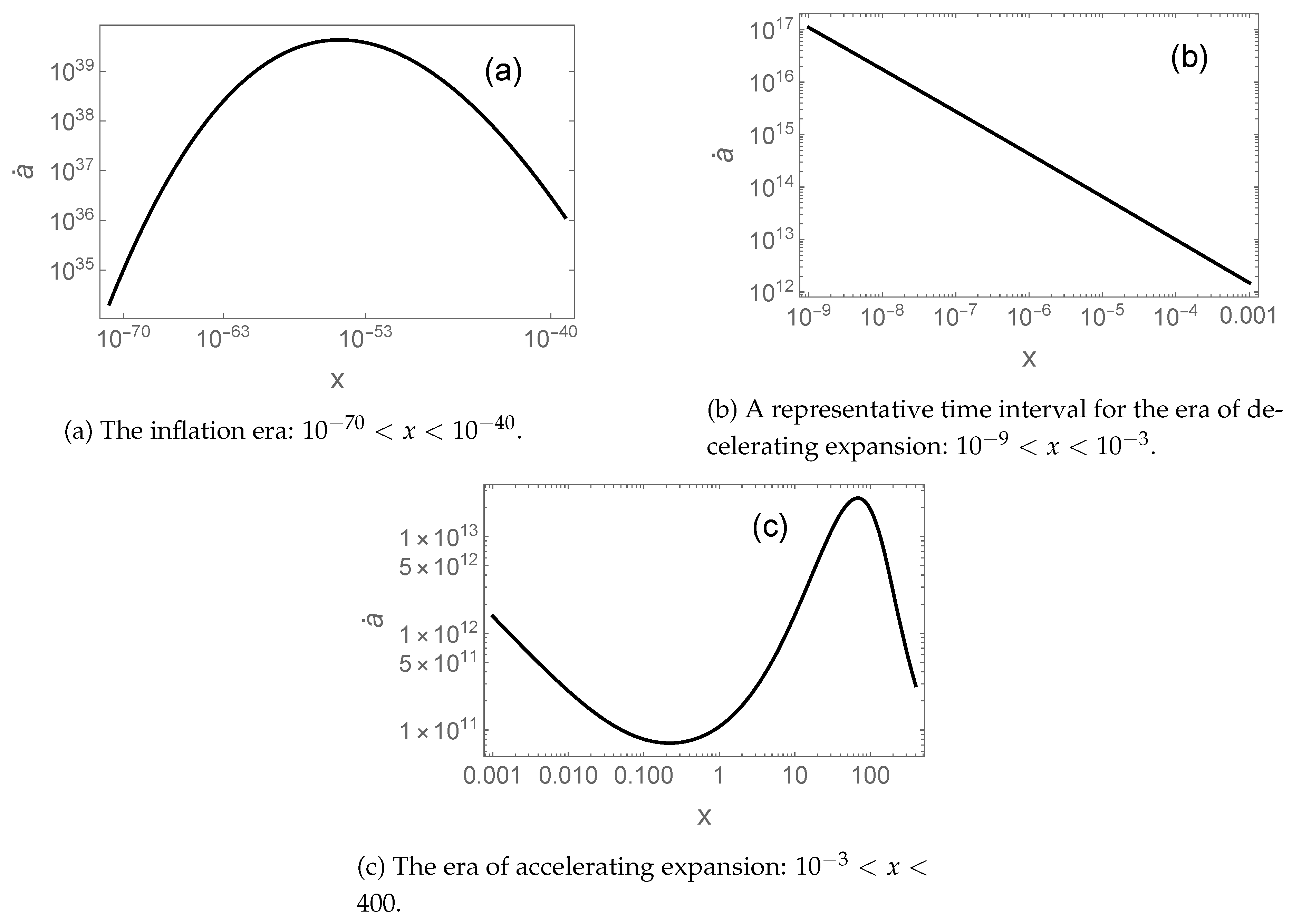

Table 1.
Comparison of cosmological parameters across three models.
| Parameter | CDM | CCC+TL | OM | Unit |
|---|---|---|---|---|
| 72 | 72.6 | 72 | ||
| -0.64 | -0.78 | -0.69 | NA | |
| 13.8 | 26.7 | 34.5 | Gyr | |
| 0.03 | Gyr | |||
| 0.5 | 5.8 | 11.5 | Gyr | |
| 0.2 | 3.5 | 7.8 | Gyr |
Disclaimer/Publisher’s Note: The statements, opinions and data contained in all publications are solely those of the individual author(s) and contributor(s) and not of MDPI and/or the editor(s). MDPI and/or the editor(s) disclaim responsibility for any injury to people or property resulting from any ideas, methods, instructions or products referred to in the content. |
© 2025 by the authors. Licensee MDPI, Basel, Switzerland. This article is an open access article distributed under the terms and conditions of the Creative Commons Attribution (CC BY) license (http://creativecommons.org/licenses/by/4.0/).
Copyright: This open access article is published under a Creative Commons CC BY 4.0 license, which permit the free download, distribution, and reuse, provided that the author and preprint are cited in any reuse.


