
Submitted:
26 January 2025
Posted:
28 January 2025
You are already at the latest version
Abstract
The differential quasilinearization method (DQM) is presented as an effective technique for obtaining approximate analytical solutions to ordinary differential equations (ODEs). This method converts general ODEs into a sequence of linear ODEs, facilitating efficient computation of successive approximations. As demonstrated by examples in the text, DQM is especially well-suited for addressing implicit or nonlinear ODEs.
Keywords:
differential quasilinearization method
; ODEs
; successive approximation methods
1. Introduction
It is often challenging to obtain analytical solutions to ordinary differential equations (ODEs), leading to the development of various methods for finding approximate solutions1–10. These approximation methods can be categorized into two main types: numerical methods and analytical methods. Analytical methods, in particular, are widely used in solving many scientific and engineering problems due to their straightforward formulation, good continuity, and clearer physical interpretation.
Among the analytical methods, successive approximation techniques are especially valued for their simplicity, broad applicability, and controllable accuracy. As a result, they have garnered increasing attention from researchers across various fields. Notable successive approximation methods include the Picard iteration method5,11,12, the Adomian decomposition method (ADM) 6,7,13–16, the homotopy analysis method (HAM) 8,17–21, the variational iteration method (VIM) 10,22–25, and the quasilinearization method 12. However, these methods typically require that the equation(s) be explicit or have a linear differential operator, that is, the equation(s) can be written in the following form
where is a linear differential operator and is either a linear or nonlinear operator. For example, consider the equation:
In this case, the linear differential operator can be expressed as:
The operator can be expressed as:
Similarly, for the equation:
The linear differential operator can be expressed as:
The operator can be expressed as:
In this work, the differential quasilinearization method (DQM), free from the previously mentioned limitations, is presented for solving initial value problems of ordinary differential equations (ODEs), especially for implicit or nonlinear cases. The validity of this method are verified through two examples.
2. The basic principle of differential quasilinearization method
2.1. Quasilinearization of ordinary differential equations
To illustrate the basic concept of the DQM, we consider the following general system of ODEs:
subject to the initial condition:
where:
and are considered as column vectors. Taking the derivative of both sides of Equation (2.1), we obtain:
If the and are regarded as known functions with respect to , Equation (2.5) can be treated as a system of linear ODEs. Consequently, the initial value problem described by Equations (2.1) and (2.2) is converted to the initial value problem of ODEs with a linear differential operator, as follows:
The existence and uniqueness of the solution to the initial value problem (2.6) can be determined by the principle of contraction mapping or the Picard–Lindelöf theorem11. Successive approximations of the solution can then be obtained using the Picard iteration method or other established methods applicable to ODEs with a linear part11.
2.2. Quasilinearization recursion equations of ODEs
To solve the initial value problem described by Equation (2.6), we aim to construct a sequence of vector-valued functions that converges to the solution of this initial value problem, such that:
where:
By substituting the components of with the components in the corresponding dimension of element(s) in , a recurrence equation based on Equation (2.8) can be obtained:
where:
Each term in the sequence can typically be deduced successively. It is important to note that in Equation (2.12), the largest subscript of in and must be smaller than . In addition, the elements of must satisfy the initial conditions:
and an initial guess for is required. By substituting the known elements of with smaller subscripts (, , …, ) into the recursive Equation (2.12), the Equation can be viewed as a linear Equation with respect to Thus, can typically be obtained by solving a system of linear differential equations. Repeating this process allows us to obtain any term in the sequence . If the initial value problem described by Equation (2.6) has a unique solution, can be regarded as an approximate solution to the initial value problem.
3. A simplified version of the differential quasilinearization method: converting to lower-order quasilinear ODEs and recursive equations
3.1. General system of ODEs
Even linear ODEs can be challenging to solve when the order is relatively high, although they are generally simpler than nonlinear ODEs. To simplify the problem, Equation (2.5) can be transformed into a system of lower-order ODEs, ideally first-order ODEs.
Let:
then:
Thus, Equation (2.5) can be converted into the following first-order ODEs:
and the initial value problem expressed in Equation (2.6) can be transformed into:
where the expressions for and are shown in Equations (3.2) and (3.3), respectively. Next, proceed with the method outlined in last section for further processing. To provide a more intuitive introduction to the simplified version of DQM, first-order ODE and system of first-order ODEs will be used as examples for a more detailed discussion in the following sections.
3.2. First order ODE
For example, consider the ODE:
subject to the initial condition:
where has continuous partial derivatives with respect to , and , and has continuous second derivatives.
The solution can be found by combining Equations (3.6) and (3.7):
If the solution is not unique, separate cases need to be considered. Taking the derivative of both sides of Equation (3.6), we obtain:
Let
then Equation (3.9) can be rewritten as:
If:
then from Equation (3.11), it follows that:
For points that do not satisfy Inequality (3.12), from the previous continuity condition, the left side of Equation (3.13) equals the limit of the right side as approaches the corresponding points. Let:
Equations (3.10) and (3.13) form a system of differential equations that can be expressed in vector notation as:
Let:
According to Equations (3.7), (3.10), and (3.14), we have
Hence, the initial value problem described by Equations (3.6) and (3.7) is transformed into:
The Picard–Lindelöf theorem provides the conditions under which the initial value problem described by Equation (3.18) has a unique solution, and successive approximations of the solution can be obtained using the Picard iteration method11.
3.3. System of first order ODEs
Consider the system of ODEs:
subject to the initial conditions:
where and have continuous partial derivatives with respect to and both and have continuous second derivatives.
From Equations (3.19) and (3.20), we obtain:
These equations can be solved to find:
Similar to the case discussed in last subsection, if the solution is not unique, separate cases need to be considered. Differentiating both sides of Equation (3.19), we get:
Let:
Substituting these into Equation (3.23), we can rewrite it as:
If:
then Equation (3.25) can be solved to find:
Similar to the situation in last subsection, for points that do not satisfy Inequality (3.26), the left side of Equation (3.27) equals the limit of the right side as approaches these points, as guaranteed by the continuity conditions. This same principle applies to similar scenarios later on.
Define:
where and . Based on Equations (3.20), (3.22), (3.24), (3.27), and (3.28), the initial value problem described by Equations (3.19) and (3.20) can be transformed into the following initial value problem in vector form:
The Picard–Lindelöf theorem provides the conditions under which the initial value problem in Equation (3.29) has a unique solution, and successive approximations of the solution can be obtained using the Picard iteration method11.
4. Existence and uniqueness of solutions
Definition 1 (Lipschitz condition)11 A vector function is said to satisfy a uniform Lipschitz condition with respect to on the open set provided there is a constant such that:
for all . The constant is called a Lipschitz constant for with respect to on .
Theorem 1 (Picard-Lindelöf theorem)11 Assume that is a continuous vector function on the rectangle:
and that satisfies a uniform Lipschitz condition with respect to on . Let:
Then the initial value problem described by Equations (3.18) and (3.29) has a unique solution on .
According to Picard iteration method, the sequence defined as:
converges uniformly to the unique solution of the initial value problem described by Equations (3.18) and (3.29) over the interval , and:
where is a Lipschitz constant. Hence, can be regarded as an approximate solution to the initial value problem, and the error can be estimated using equation (3.34).
5. Examples
5.1. First order ODE
Consider the following initial value problem for the ODE:
where has continuous second derivative.
From Equation (4.1), we obtain:
Combining Equations (4.1) and (4.2), we solve:
By differentiating both sides of the ODE in Equation (4.1), we get:
Using the continuity condition, we derive:
Let:
The initial value problem described by Equation (4.1) is then transformed into:
where:
When:
According to Equation (3.33), we can calculate:
It is not difficult to prove that:
which implies:
Similarly, when:
we obtain:
In conclusion, the solution to the initial value problem described by Equation (4.1) is
This solution can be easily obtained or verified by other methods. The approximate analytical solutions of Equation (4.1) using the DQM and the exact solution are plotted in Figure 1. As seen in the figure, the approximate solution is already very close to the exact solution.
5.2. System of first order ODEs
Consider an object of mass moving in a uniform circle under the gravitational pull of another object with mass located at the origin , where is the gravitational constant. The initial position of the orbiting object is . The goal is to determine the position coordinates of this object at any time.
Let represent the coordinates of the object at time . The zero potential energy point is selected at infinity. Using the principles of energy conservation and angular momentum conservation, the following ODEs and initial conditions can be derived:
where and are functions of . From Equation (4.16), we find:
Taking the derivatives of both sides of the ODEs in Equation (4.16), we obtain:
Using the continuity condition, we derive:
Let:
The initial value problem described by Equation (4.16) is then transformed into:
where:
Using Equation (3.33), we obtain:
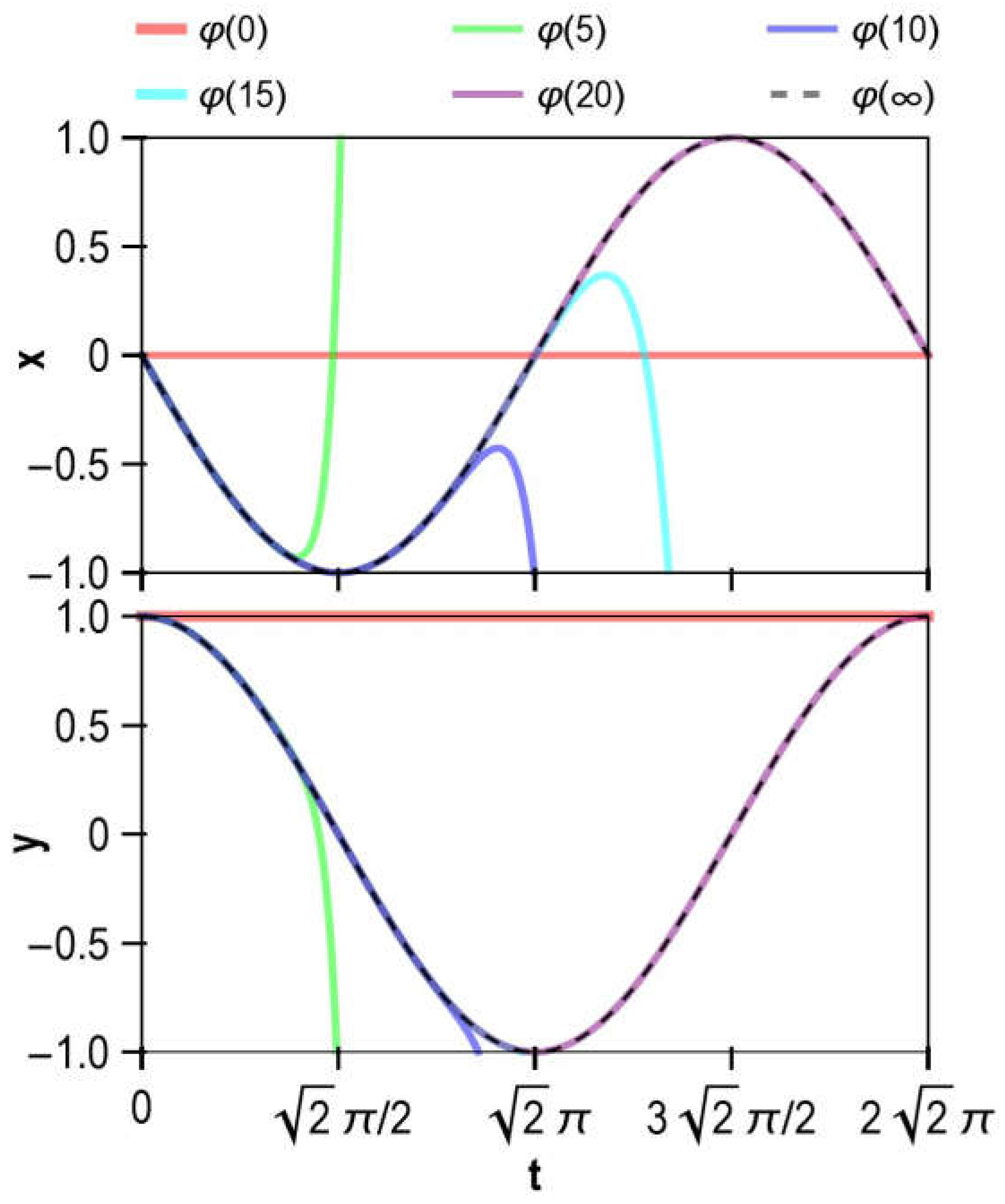
For convenience, terms in the sequence that exceed the 20th power are excluded from the calculation in Equation (4.23); however, this approach may lead to different convergence speeds. From a physical standpoint, it is straightforward to show that the solution to the initial value problem described by Equation (4.16) is:
The approximate analytical solutions of Equation (4.16), obtained via the DQM, along with the exact solution, are plotted in Figure 2. As observed from the figure, within the interval , the approximate solution closely matches the exact solution.
6. Conclusion
The differential quasilinearization method (DQM) for obtaining approximate analytical solutions of ordinary differential equations (ODEs) was presented in this study. DQM is a widely applicable approach for solving initial value problems of ODEs, especially well-suited for addressing implicit or nonlinear ODEs. The effectiveness of this method was verified by solving specific examples of both single ODE and system of ODEs.
References
- Michoski, C., Milosavljević, M., Oliver, T. & Hatch, D. R. Solving differential equations using deep neural networks. Neurocomputing 399, 193–212 (2020). [CrossRef]
- Kojouharov, H. V, Roy, S., Gupta, M., Alalhareth, F. & Slezak, J. M. A second-order modified nonstandard theta method for one-dimensional autonomous differential equations. Appl. Math. Lett. 112, 106775 (2021). [CrossRef]
- Fekete, I., Conde, S. & Shadid, J. N. Embedded pairs for optimal explicit strong stability preserving Runge–Kutta methods. J. Comput. Appl. Math. 412, 114325 (2022). [CrossRef]
- Dwivedi, V. & Srinivasan, B. Physics Informed Extreme Learning Machine (PIELM)–A rapid method for the numerical solution of partial differential equations. Neurocomputing 391, 96–118 (2020).
- Ramos, J. I. On the Picard–Lindelof method for nonlinear second-order differential equations. Appl. Math. Comput. 203, 238–242 (2008). [CrossRef]
- Chen, F. & Liu, Q. Modified asymptotic Adomian decomposition method for solving Boussinesq equation of groundwater flow. Appl. Math. Mech. Ed. 35, 481–488 (2014). [CrossRef]
- Li, W. & Pang, Y. Application of Adomian decomposition method to nonlinear systems. Adv. Differ. Equations 2020, 67 (2020). [CrossRef]
- Shukla, A. K., Ramamohan, T. R. & Srinivas, S. Homotopy analysis method with a non-homogeneous term in the auxiliary linear operator. Commun. Nonlinear Sci. Numer. Simul. 17, 3776–3787 (2012). [CrossRef]
- Ghoreishi, M., Ismail, A. I. B. M., Alomari, A. K. & Sami Bataineh, A. The comparison between Homotopy Analysis Method and Optimal Homotopy Asymptotic Method for nonlinear age-structured population models. Commun. Nonlinear Sci. Numer. Simul. 17, 1163–1177 (2012). [CrossRef]
- He, J. & Wu, X. Variational iteration method: New development and applications. Comput. Math. with Appl. 54, 881–894 (2007). [CrossRef]
- Kelley, W. G. & Peterson, A. C. The Theory of Differential Equations: Classical and Qualitative. (Springer, 2010).
- Pandey, R. K. & Tomar, S. An effective scheme for solving a class of nonlinear doubly singular boundary value problems through quasilinearization approach. J. Comput. Appl. Math. 392, 113411 (2021). [CrossRef]
- Turkyilmazoglu, M. Accelerating the convergence of Adomian decomposition method (ADM). J. Comput. Sci. 31, 54–59 (2019). [CrossRef]
- Zeidan, D., Chau, C. K., Lu, T.-T. & Zheng, W.-Q. Mathematical studies of the solution of Burgers’ equations by Adomian decomposition method. Math. Methods Appl. Sci. 43, 2171–2188 (2020). [CrossRef]
- Duan, J.-S., Chaolu, T., Rach, R. & Lu, L. The Adomian decomposition method with convergence acceleration techniques for nonlinear fractional differential equations. Comput. Math. with Appl. 66, 728–736 (2013). [CrossRef]
- Aly, E. H., Ebaid, A. & Rach, R. Advances in the Adomian decomposition method for solving two-point nonlinear boundary value problems with Neumann boundary conditions. Comput. Math. with Appl. 63, 1056–1065 (2012).
- Naik, P. A., Zu, J. & Ghoreishi, M. Estimating the approximate analytical solution of HIV viral dynamic model by using homotopy analysis method. Chaos, Solitons & Fractals 131, 109500 (2020). [CrossRef]
- Rana, P., Shukla, N., Gupta, Y. & Pop, I. Homotopy analysis method for predicting multiple solutions in the channel flow with stability analysis. Commun. Nonlinear Sci. Numer. Simul. 66, 183–193 (2019). [CrossRef]
- Motsa, S. S., Sibanda, P. & Shateyi, S. A new spectral-homotopy analysis method for solving a nonlinear second order BVP. Commun. Nonlinear Sci. Numer. Simul. 15, 2293–2302 (2010). [CrossRef]
- Liao, S. On the relationship between the homotopy analysis method and Euler transform. Commun. Nonlinear Sci. Numer. Simul. 15, 1421–1431 (2010). [CrossRef]
- Abidi, F. & Omrani, K. The homotopy analysis method for solving the Fornberg–Whitham equation and comparison with Adomian’s decomposition method. Comput. Math. with Appl. 59, 2743–2750 (2010). [CrossRef]
- He, J. Variational iteration method—Some recent results and new interpretations. J. Comput. Appl. Math. 207, 3–17 (2007). [CrossRef]
- Anjum, N. & He, J. Laplace transform: Making the variational iteration method easier. Appl. Math. Lett. 92, 134–138 (2019).
- Torsu, P. On variational iterative methods for semilinear problems. Comput. Math. with Appl. 80, 1164–1175 (2020). [CrossRef]
- Nadeem, M., Li, F. & Ahmad, H. Modified Laplace variational iteration method for solving fourth-order parabolic partial differential equation with variable coefficients. Comput. Math. with Appl. 78, 2052–2062 (2019). [CrossRef]
Figure 1.
Graphs of the approximate analytical solutions of Equation (4.1) obtained using the DQM compared with the exact solution.
Figure 1.
Graphs of the approximate analytical solutions of Equation (4.1) obtained using the DQM compared with the exact solution.
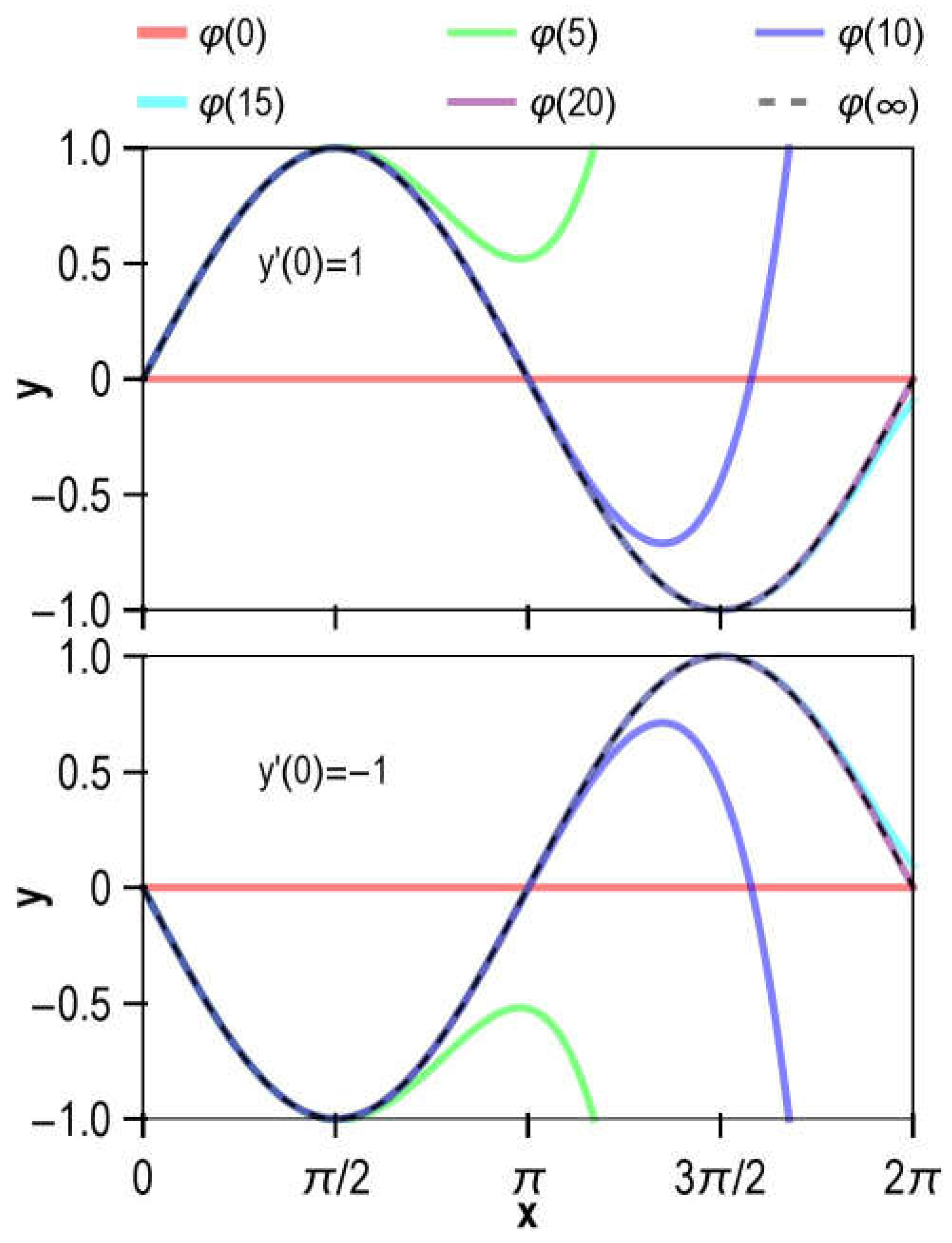
Figure 2.
Graphs of the approximate analytical solutions of Equation (4.16) obtained using the DQM compared with the exact solution.
Figure 2.
Graphs of the approximate analytical solutions of Equation (4.16) obtained using the DQM compared with the exact solution.
Disclaimer/Publisher’s Note: The statements, opinions and data contained in all publications are solely those of the individual author(s) and contributor(s) and not of MDPI and/or the editor(s). MDPI and/or the editor(s) disclaim responsibility for any injury to people or property resulting from any ideas, methods, instructions or products referred to in the content. |
© 2025 by the authors. Licensee MDPI, Basel, Switzerland. This article is an open access article distributed under the terms and conditions of the Creative Commons Attribution (CC BY) license (http://creativecommons.org/licenses/by/4.0/).
Copyright: This open access article is published under a Creative Commons CC BY 4.0 license, which permit the free download, distribution, and reuse, provided that the author and preprint are cited in any reuse.


