
Submitted:
23 January 2025
Posted:
24 January 2025
You are already at the latest version
Abstract
During the past decades, delayed differential dynamical equation has displayed a great application in
portraying the interplay of diverse chemical substances in chemistry.
In the research, relying the earlier publications, we propose a novel nutrient-microorganism system accompanying time delay.
Exploiting fixed point theorem, inequality skills and a proper function, we
acquire the parameter criteria on well-posedness (for example, existence and uniqueness, non-negativeness and boundedness) of the solution of the established delayed nutrient-microorganism system.
Utilizing Hopf bifurcation theory and stability criterion of delayed dynamical system, we deal with the onset of Hopf bifurcation phenomenon and stability trait
of the established delayed nutrient-microorganism system. A set of novel delay-independent parameter conditions on
bifurcation phenomenon and stability of the system are provided. Designing both different hybrid delayed feedback controllers,
we have successfully controlled the time of occurrence of bifurcation phenomenon and stability domain of the system.
The role of time delay in controlling bifurcation and stabilizing system is analyzed. Numerical experiment figures are given to support the gained primary outcomes.
The acquired assertions of this research are completely innovative and can give some important instructions in
regulating and balancing the densities of microorganism and nutrient.
Keywords:
nutrient-microorganism system
; well-posedness
; hopf bifurcation
; stability
; hybrid controller
; delay
MSC: 34C23; 34K18; 37GK15; 39A11; 92B20
1. Introduction
In the sediment of ocean, a great deal of chemical substances and microorganism will appear and they are closely related to each other, which formulate various intricate networks. Thus exploring the law of interaction among them is a very complex problem. In order to reveal the inherent law of chemical substances and microorganism, a lot of works on chemical substances and microorganism have been carried out. For example, Gao et al. [1] explored the spatiotemporal pattern formation and global existence of a nutrient-microorganism system involving nutrient-taxis in the sediment. Baurmann and Feudel [2] investigated the turing patterns of a nutrient-microorganism model. Cao and Wu [3] dealt with the global bifurcation and local bifurcation of both positive constant solutions of a diffusive nutrient-microorganism model. For more concrete contents, one can see [4-8].
In 2004, Baurmann and Feudel [9] proposed the following nutrient-microorganism system:
where stands for the density of microorganism and stands for the density of one chemical species in the sediment. The bacteria includes two parts (active part and inactive part). stands for the active part bacterium, it grows by feeding on the nutrient with the rate . Noticing that , we let , where denotes a constant. m denotes the bacterium mortality. The input of nutrient into the system principally derives from the seawater via the surface of sediment by applying bioirrigation which is describe by , where stands for the hydraulic conductivity between seawater and sediment, and represents the concentration of nutrient in the seawater. denotes the capture rate. For more detailed implication of system (1.1), one can see [1]. Applying the following nondimensionalizing variable substitutions:
we get
where . In many cases, the density of microorganism and the density of one chemical species in the sediment depend on the development of the current time and the past history. Here we assume that the density of microorganism depends on the current time and the past history, i.e, there is feedback delay for the variation of the density of microorganism. Relying on this viewpoint, we formulate the following delayed nutrient-microorganism system:
where is a delay. All the parameters in system (1.4) are positive real numbers.
Generally speaking, delay plays a vital role in affecting the dynamical phenomenon of differential dynamical systems. In numerous situations, delay usually leads to change of stability, onset of bifurcation phenomenon and the emergence of chaos and so on [10-21]. Especially, delay-driven bifurcation phenomenon is a vital dynamical behavior. Chemically, delay-driven bifurcation phenomenon is able to efficaciously describe the balanced relations among the concentrations of various chemical substances. As a result, it is of importance to focus on the delay-driven bifurcation phenomenon for various chemical reaction systems and biological models. Stimulated by this viewpoint above, we will deal with the delay-driven bifurcation phenomenon and bifurcation control aspect for model (1.4). In particular, we will focus on the following key issues: (a) Explore the well-posedness (e.g., boundedness, existence and uniqueness, non-negativeness) of solution of model (1.4). (b) Investigate the onset of bifurcation phenomenon and stability behavior of model (1.4). (c) Design two differential controllers to adjust the stability domain and the time of appearance of bifurcation phenomenon of system (1.4).
The main luminescent spot of this work are summarized as follows: (I) Relying on the earlier studies, a novel stability and bifurcation condition without depending on delay for model (1.4) is formulated. (II) Taking advantage of both different hybrid controllers, stability range and the time of onset of bifurcation phenomenon of model (1.4) are successfully adjusted. (III) The effect of delay on controlling bifurcation behavior and stabilizing the density of microorganism and the density of one chemical species in the sediment of model (1.4) is provided.
This organization of this study is provided as follows. The well-posedness including boundedness, existence and uniqueness and non-negativeness of the solution to model (1.4) is analyzed in “Well-posedness" section. “Bifurcation phenomenon" section studies the Hopf bifurcation issue and stability trait of system (1.4). “Bifurcation control via hybrid delayed feedback controller" section deals with the control issue of Hop bifurcation for system (1.4) by designing a proper hybrid delayed feedback controller including parameter perturbation with delay and state feedback. “Bifurcation control via extended hybrid delayed feedback controller" section focuses on the control issue of Hopf bifurcation for system (1.4) by designing a proper extended hybrid delayed feedback controller including parameter perturbation with delay and state feedback. “Numerical experiments" implements software experiments to check the effectiveness of the gained primary outcomes. A concise conclusion is given to end this article in “Conclusions".
2. Well-Posedness
In this section, we are going to explore the well-posedness of solution of model (1.4)(involve non-negativeness, existence and uniqueness and boundedness) by utilizing fixed point theory, inequality tactics and establishment of an appropriate function.
Theorem 1.
Denote , where U denotes a positive constant. For every , model (1.4) under the initial value possesses a unique solution
Proof.
Let
where
For each , one acquires
where
Set
Then by (2.3), one gets
Then conforms to Lipschitz condition concerning (see [22]). By exploiting fixed point theorem, we can lightly acquire that Theorem 2.1 holds. □
Theorem 2.
Suppose that , then every solution of system (1.4) beginning with is non-negative.
Proof.
Let be the initial condition of system (1.4). If there exists a real constant conforming to such that
By applying model (1.4), one acquires
By using Lemma 1 of Das et al. [23], we know that , which implies a contradiction (see (2.7)). Then for Using the same scheme, one can lightly know that for □
Theorem 3.
If , then all solutions to model (1.4) starting with are uniformly bounded.
Proof.
Set
Then
Making use of Gronwall’s inequality [24], one gains
The proof of Theorem 2.3 ends.
□
3. Bifurcation Phenomenon
Assume that is the equilibrium point of model (1.4), then obey
The linear equation of model (1.4) at is given by
where
The characteristic equation of system (3.2) reads as
which results in
where
When then Equation (3.5) takes the following expression:
If
is fulfilled, then the two roots and of Eq. (3.7) admit negative real parts. So one can know that the equilibrium point of model (1.4) under the time delay preserves locally asymptotically stable form.
If is the root of Eq. (3.5), then according to Equation (3.5), one gets
which generates
In view of (3.9), we gain
which results in
Denote
Notice that and , then we acquire that Eq. (3.11) owns at least one real positive root. Then Equation (3.5) admits at least one pair of purely roots. Without loss of generality, assume that Eq. (3.11) has four real positive roots (say . By (3.9), we gain
where Set and then if , (3.5) has a pair of imaginary roots .
Now we give the assumption as follows:
where
Lemma 1.
If is a root of Eq. (3.5) at obeying , then
Proof.
Based on Equation (3.5), one gains
which generates
where
Then
In view of , one gains
The proof finishes. □
Relying on the analysis above, the following outcome is lightly acquired.
Theorem 4.
If and are fulfilled, then the equilibrium point of model (1.4) keeps locally asymptotically stable condition if and model (1.4) produces a cluster of periodic solutions (namely, Hopf bifurcations) near the equilibrium point when
4. Bifurcation Control via Hybrid Delayed Feedback Controller
In this section, we are to use a hybrid controller (include a state feedback and parameter perturbation) to the first equation of model (1.4). By virtue of this controller, we can dominate the time of emergence of bifurcation phenomenon and stability region of system (1.4). Relying on the ideas of [25-29], we formulate the following fractional controlled nutrient-microorganism system:
where represents feedback gain coefficient. Model (4.1) owns the same equilibrium point as that of model (1.4). The linear equation of model (4.1) at is given by
where
The characteristic equation of system (4.2) reads as
which results in
where
When then Equation (4.5) takes the following expression:
If
is fulfilled, then the two roots and of Eq. (4.7) admit negative real parts. So one can understand that the equilibrium point of model (4.1) under the time delay preserves locally asymptotically stable form.
If is the root of Eq. (4.5), then according to Equation (4.5), one gets
which generates
In view of (4.9), we gain
which results in
Denote
Notice that and , then we acquire that Eq. (4.11) owns at least one real positive root. Then Equation (4.5) admits at least one pair of purely roots. Without loss of generality, assume that Eq. (4.11) has four real positive roots (say . By (4.9), we gain
where Set and then if , (4.5) has a pair of imaginary roots .
Now we give the assumption as follows:
where
Lemma 2.
If is a root of Eq. (4.5) at obeying , then
Proof.
Based on Equation (4.5), one gains
which generates
where
Then
In view of , one gains
The proof finishes. □
Relying on the analysis above, the following outcome is lightly acquired.
Lemma 3.
If and are fulfilled, then the equilibrium point of model (4.1) keeps locally asymptotically stable condition if and model (4.1) produces a cluster of periodic solutions (namely, Hopf bifurcations) near the equilibrium point when
5. Bifurcation Control via Extended Hybrid Delayed Feedback Controller
In this section, we are to use two hybrid controllers (include a state feedback and parameter perturbation) to the both equations of model (1.4). By virtue of the two controllers, we can dominate the time of emergence of bifurcation phenomenon and stability region of system (1.4). Relying on the ideas of [25-29], we formulate the following fractional controlled nutrient-microorganism system:
where represent feedback gain parameters. Clearly, system (5.1) and system (1.5) admit the mutual equilibrium point . The linear equation for system (5.1) at is given by
where
The characteristic equation of system (5.2) reads as
which results in
where
When then Equation (5.5) owns the following expression:
If
is fulfilled, then the two roots of Eq. (5.7) admit negative real parts. So one can conclude that the equilibrium point of system (5.1) under the time delay keeps locally asymptotically stable level.
By (5.5), we have
Let be the root of Eq. (5.8). By Eq. (5.8), we get
which results in
By (5.10), one gains
In view of , we get
which results in
where
Define
Suppose that
holds, notice that , then one understands that Eq. (5.13) admits at least one real positive root. So Equation (5.5) owns at least one pair of purely roots. Without loss of generality, assume that Eq. (5.13) admits eight real positive roots (say . According to (5.11), we gain
where Let and assume that when , (5.5) admits a pair of imaginary roots .
Next the following condition is given:
where
Lemma 4. Lemma 5.1.
If is a root of Eq. (5.5) near that obeys , then
Proof.
By virtue of Equation (5.5), one gains
which results in
where
Then
In view of , one gains
The proof completes. □
Depending on the discussion above, the following outcome is lightly acquired.
Theorem 5.
If - are satisfied, then the equilibrium point of system (5.1) keeps locally asymptotically stable level if and model (5.1) produces a cluster of periodic solutions (i.e., Hopf bifurcations) near the equilibrium point when
6. Numerical Experiments
Example 1.
Consider the following delayed nutrient-microorganism system:
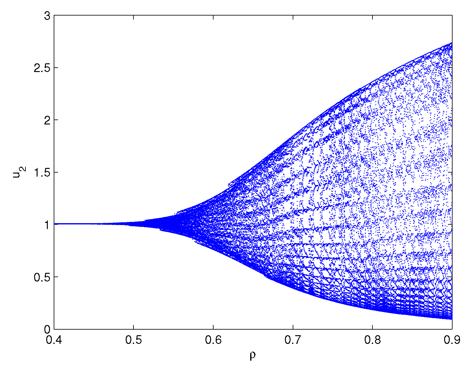
One can lightly acquire that model (6.1) owns the positive equilibrium point . By a series of algebraic operation, we can verify that the three assumptions of Theorem 3.1 hold true. Using Matlab software, one gains . In order to check the onset of Hopf bifurcation and stability issue of Theorem 3.1, both unequal delay values are provided. On the one hand, we select which demonstrates , namely, ρ is located within the range . On the other hand, we select which demonstrates , namely, ρ is located outside of the range . For , we obtain the simulation Figure 1. Based on Figure 1, we can lightly see that the positive equilibrium point is locally stable. In other words, the density of microorganism and the density of one chemical species in the sediment will run towards respectively. For , we obtain the simulation Figure 2. Based on Figure 2, we can lightly see that a family of periodic solutions (i.e, Hopf bifurcations) will take place around positive equilibrium point . In other words, the density of microorganism and the density of one chemical species in the sediment will retain periodic vibration around the values respectively. In addition, to show visually the bifurcation point, we draw the corresponding bifurcation diagrams which are given in Figure 3 and Figure 4. One can know that the bifurcation value is about .
Example 2.
Consider the following controlled delayed nutrient-microorganism system:
One can lightly acquire that model (6.2) owns the positive equilibrium point . Let . By a series of algebraic operation, we can verify that the three assumptions of Theorem 4.1 hold true. Using Matlab software, one gains . In order to check the onset of Hopf bifurcation and stability issue of Theorem 4.1, both unequal delay values are provided. On the one hand, we select which demonstrates , namely, ρ is located within the range . On the other hand, we select which demonstrates , namely, ρ is located outside of the range . For , we obtain the simulation Figure 5. Based on Figure 5, we can lightly see that the positive equilibrium point is locally stable. In other words, the density of microorganism and the density of one chemical species in the sediment will run towards respectively. For , we obtain the simulation Figure 6. Based on Figure 6, we can lightly see that a family of periodic solutions (i.e, Hopf bifurcations) will take place around positive equilibrium point . In other words, the density of microorganism and the density of one chemical species in the sediment will retain periodic vibration around the values respectively. In addition, to show visually the bifurcation point, we draw the corresponding bifurcation diagrams which are given in Figure 7 and Figure 8. One can know that the bifurcation value is about .
Example 3.
Consider the following controlled delayed nutrient-microorganism system:
One can lightly acquire that model (6.3) owns the positive equilibrium point . Let . By a series of algebraic operation, we can verify that the three assumptions of Theorem 5.1 hold true. Using Matlab software, one gains . In order to check the onset of Hopf bifurcation and stability issue of Theorem 5.1, both unequal delay values are provided. On the one hand, we select which demonstrates , namely, ρ is located within the range . On the other hand, we select which demonstrates , namely, ρ is located outside of the range . For , we obtain the simulation Figure 9. Based on Figure 9, we can lightly see that the positive equilibrium point is locally stable. In other words, the density of microorganism and the density of one chemical species in the sediment will run towards respectively. For , we obtain the simulation Figure 10. Based on Figure 10, we can lightly see that a family of periodic solutions (i.e, Hopf bifurcations) will take place around positive equilibrium point . In other words, the density of microorganism and the density of one chemical species in the sediment will retain periodic vibration around the values respectively. In addition, to show visually the bifurcation point, we draw the corresponding bifurcation diagrams which are given in Figure 11 and Figure 12. One can know that the bifurcation value is about .
Remark 1.
Relying on the numerical simulation outcomes in Example 6.1-Example 6.3, we can find that system (6.1) owns the bifurcation value , system (6.2) owns the bifurcation value , system (6.3) owns the bifurcation value , which confirms that we can postpone the time of appearance of bifurcation phenomenon of system (6.1) and expand the stability range of system (6.1) via our designed both different hybrid delayed feedback controllers in varying degrees.
7. Conclusions
During the past decades, mathematical models play a vital role in depicting the evolution of various chemical compositions in chemical reactions. Various chemical reaction models have been formulated and a lot of dynamical behavior of these chemical reaction models have been studied. In the manuscript, based on the forefathers’ research, we build new delayed nutrient-microorganism system. The parameter conditions on the existence and uniqueness, non-negativeness and boundedness of the solution of this model are acquired via fixed point theorem, inequality technique and a reasonable function. The stability and bifurcation phenomenon are discussed by virtue of the stability criterion and bifurcation argument of fractional delayed dynamical system. The critical delay value to guarantee the onset of Hopf bifurcation of this model is acquired. In order to control the the time of emergence of bifurcation phenomenon and stability domain of this model, two different hybrid controllers are provided to achieve the our goal. In these controllers, we can find that delay and control parameters are very important factors in achieve the our goal. The research fruits own enormous theoretical significance in dominating and optimizing the densities of microorganism and nutrient. Also the research fruits can be applied to control the stability, bifurcation behavior and chaos in many differential dynamical models (include integer-order and fractional-order dynamical models) in lots of areas.
Data Availability Statement
No data were used to support this study.
Acknowledgments
This work is supported by Natural Science Foundation of Henan Province(No.242300420242) and Innovative Exploration and New Academic talent project of Guizhou University of Finanace and Economics (No. 2024XSXMA03).
Conflicts of Interest
The authors declare that they have no conflict of interest.
References
- J.P. Gao, S.J. Guo, L. Ma, Global existence and spatiotemporal pattern formation of a nutrient-microorganism model with nutrient-taxis in the sediment, Nonlinear Dynamics 108 (2022) 4207-4229. [CrossRef]
- M. Baurmann, U. Feudel, Turing patterns in a simple model of a nutrient-microorganism system in the sediment, Ecol. Complex. 1(1) (2004) 77-94. [CrossRef]
- Q. Cao, J.H. Wu, Patterns and dynamics in the diffusive model of a nutrient–Cmicroorganism system in the sediment, Nonlinear Analysis: Real World Applications 49 (2019) 331-354. [CrossRef]
- M.X. Chen, R.C. Wu, Dynamics of diffusive nutrient-microorganism model with spatially heterogeneous environment, Journal of Mathematical Analysis and Applications 511(1) (2022) 126078. [CrossRef]
- B. Mukhopadhyay, R. Bhattacharyya, Modelling phytoplankton allelopathy in a nutrient-plankton model with spatial heterogeneity, Ecological Modelling 198 (1-2) (2006) 163-173. [CrossRef]
- M.X. Chen, R.C. Wu, B. Liu, L.P. Chen, Hopf-Hopf bifurcation in the delayed nutrient-microorganism model, Applied Mathematical Modelling 86 (2020) 460-483. [CrossRef]
- T.Y. Wang, L.S. Chen, P. Zhang, Extinction and permanence of two-nutrient and two-microorganism chemostat model with pulsed input, Communications in Nonlinear Science and Numerical Simulation 15(10) (2010) 3035-3045. [CrossRef]
- R. Liu, W.B. Ma, K. Guo, The general chemostat model with multiple nutrients and flocculating agent: From deterministic behavior to stochastic forcing transition, Communications in Nonlinear Science and Numerical Simulation 117 (2023) 106910. [CrossRef]
- M. Baurmann, U. Feudel, Turing patterns in a simple model of a nutrient-microorganism system in the sediment, Ecological Complexity 1(1) (2004) 77-94. [CrossRef]
- C.J. Xu, D. Mu, Z.X. Liu, Y.C. Pang, M.X. Liao, C. Aouiti, New insight into bifurcation of fractional-order 4D neural networks incorporating two different time delays, Communications in Nonlinear Science and Numerical Simulation 118 (2023) 107043. [CrossRef]
- C.J. Xu, D. Mu, Z.X. Liu, Y.C. Pang, M.X. Liao, P.L. Li, L.Y. Yao, Q.W. Qin, Comparative exploration on bifurcation behavior for integer-order and fractional-order delayed BAM neural networks, Nonlinear Analysis: Modelling and Control 27 (2022) 1030-1053. [CrossRef]
- C.J. Xu, M. Farman, A. Akgül, K.S. Nisar, A. Ahmad, Modeling and analysis fractal order cancer model with effects of chemotherapy, Chaos, Solitons & Fractals 161 (2022) 112325. [CrossRef]
- C.J. Xu, D. Mu, Y.L. Pan, C. Aouiti, L.Y. Yao, Exploring bifurcation in a fractional-order predator-prey system with mixed delays, Journal of Applied Analysis and Computation 13(3) (2023) 1119-1136. [CrossRef]
- C.J. Xu, Y.S. Wu, Bifurcation and control of chaos in a chemical system, Applied Mathematical Modelling 39 (8) (2015) 2295-2310. [CrossRef]
- C.J. Xu, Z.X. Liu, Y.C. Pang, S. Saifullah, M. Inc, Oscillatory, crossover behavior and chaos analysis of HIV-1 infection model using piece-wise Atangana-Baleanu fractional operator: Real data approach, Chaos, Solitons & Fractals 164 (2022) 112662. [CrossRef]
- C.J. Xu, M.X. Liao, P.L. Li, L.Y. Yao, Q.W. Qin, Y.L. Shang, Chaos control for a fractional-order Jerk system via time delay feedback controller and mixed controller, Fractal and Fractional 5(4) (2021) 257. [CrossRef]
- C.J. Xu, Z.X. Liu, P.L. Li, J.L. Yan, L.Y. Yao, Bifurcation mechanism for fractional-order three-triangle multi-delayed neural networks, Neural Processing Letters 55(9) (2023) 6125-6151. [CrossRef]
- C.J. Xu, W. Zhang, C. Aouiti, Z.X. Liu, L.Y. Yao, Bifurcation insight for a fractional-order stage-structured predator-prey system incorporating mixed time delays, Mathematical Methods in the Applied Sciences 46(8) (2023) 9103-9118. [CrossRef]
- C.J. Xu, Q.Y. Cui, Z.X. Liu, Y.L. Pan, X.H. Cui, W. Ou, M. Rahman, M. Farman, S. Ahmad, A. Zeb, Extended hybrid controller design of bifurcation in a delayed chemostat model, MATCH Communications in Mathematical and in Computer Chemistry 90(3) (2023) 609-648. [CrossRef]
- C.J. Xu, X.H. Cui, P.L. Li, J.L. Yan, L.Y. Yao, Exploration on dynamics in a discrete predator-prey competitive model involving time delays and feedback controls, Journal of Biological Dynamics 17(1)(2023) 2220349. [CrossRef]
- D. Mu, C.J. Xu, Z.X. Liu, Y.C. Pang, Further insight into bifurcation and hybrid control tactics of a chlorine dioxide-iodine-malonic acid chemical reaction model incorporating delays, MATCH Communications in Mathematical and in Computer Chemistry 89(3)(2023) 529-566. [CrossRef]
- H.L. Li, L. Zhang, C. Hu, Y.L. Jiang, Z.D. Teng, Dynamical analysis of a fractional-order prey-predator model incorporating a prey refuge, Journal of Applied Mathemtics and Computing 54 (2017) 435-449. [CrossRef]
- M. Das, A. Maiti, G.P. Samanta, Stability analysis of a prey-predator fractional order model incorporating prey refuge, Ecological Genetics and Genomics, 7-8 (2018) 33-46. [CrossRef]
- L. Li, Y.X. Zhang, Dynamic analysis and Hopf bifurcation of a Lengyel-Epstein system with two delays, Journal of Mathematics, Volume 2021, Article ID 5554562, 18 pages. [CrossRef]
- Z.Z. Zhang, H.Z. Yang, Hybrid control of Hopf bifurcation in a two prey one predator system with time delay, Proceeding of the 33rd Chinese Control Conference, July 28-30 (2014) 6895-6900. Nanjing, China. [CrossRef]
- L.P. Zhang, H.N. Wang, M. Xu, Hybrid control of bifurcation in a predator-prey system with three delays, Acta Physica Sinica 60 (1)(2011) 010506. [CrossRef]
- R.Y. Zhang, Bifurcation analysis for T system with delayed feedback and its application to control of chaos, Nonlinear Dynamics 72 (2013) 629-641. [CrossRef]
- L. Li, C.D. Huang, X.Y. Song, Bifurcation control of a fractional-order PD control strategy for a delayed fractional-order predator-prey system, The European Physical Journal Plus 138 (2023) 77. [CrossRef]
- S. Akhtar, R. Ahmed, M. Batool, N.A. Shah, J.D. Chung, Stability, bifurcation and chaos control of a discretized Leslie prey-predator model, Chaos, Solitons & Fractals 152 (2021) 111345. [CrossRef]
Figure 1.
Numerical experiment outcomes of system (6.1) involving the time delay The equilibrium point retains locally asymptotically stable condition.
Figure 1.
Numerical experiment outcomes of system (6.1) involving the time delay The equilibrium point retains locally asymptotically stable condition.
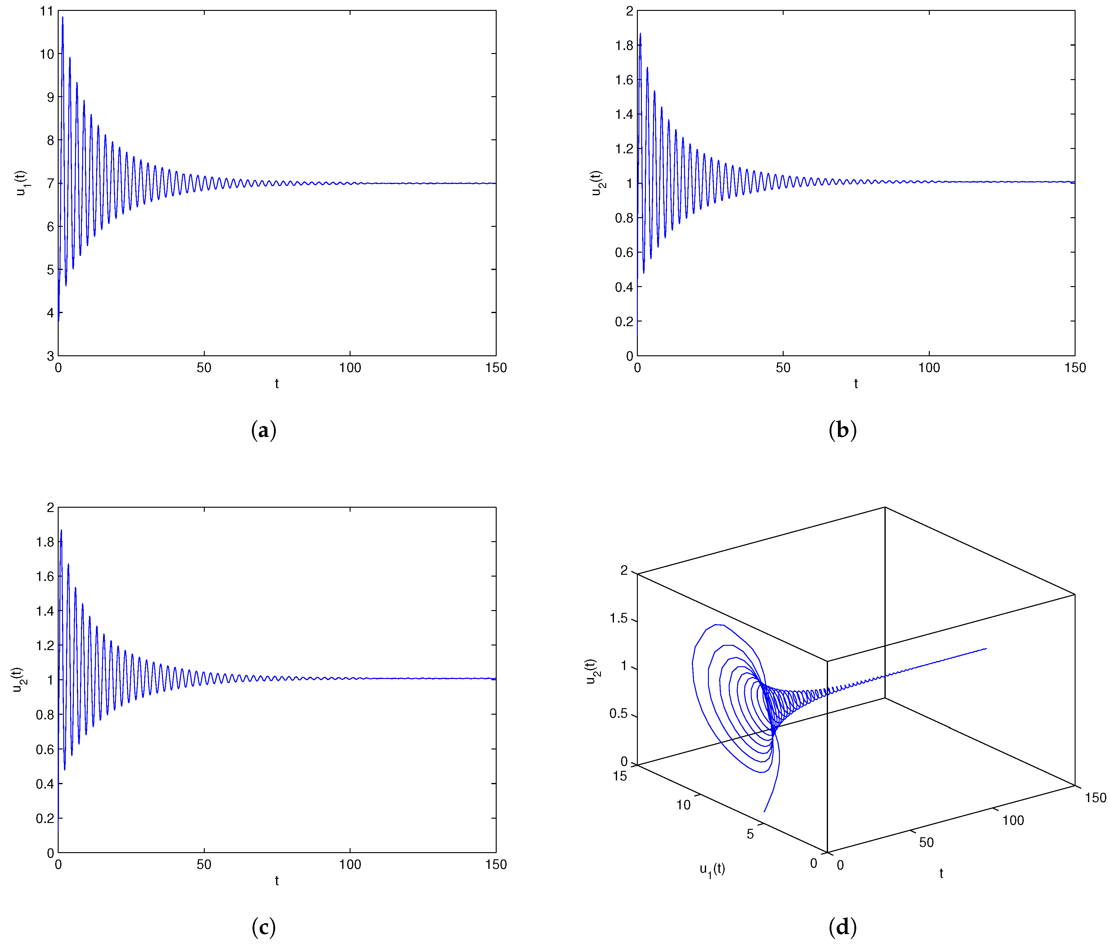
Figure 2.
Numerical experiment outcomes of model (6.1) involving the time delay A family of periodic solutions (namely, Hopf bifurcations) come into being in the nearby the equilibrium point .
Figure 2.
Numerical experiment outcomes of model (6.1) involving the time delay A family of periodic solutions (namely, Hopf bifurcations) come into being in the nearby the equilibrium point .
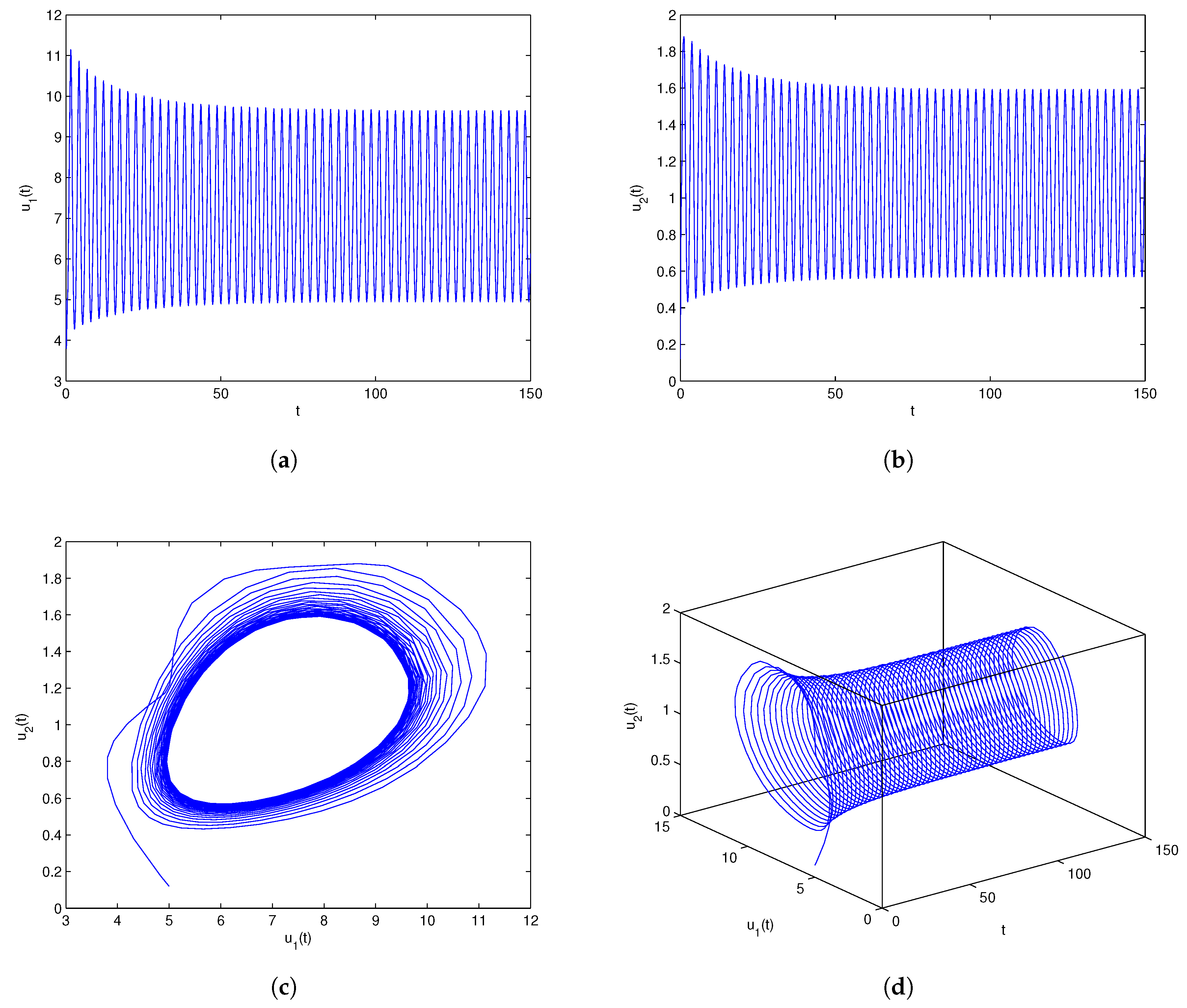
Figure 3.
Bifurcation diagram of model (6.1): x-axis represents the time delay and y-axis represents the variable . Model (6.1) admits the bifurcation value .
Figure 3.
Bifurcation diagram of model (6.1): x-axis represents the time delay and y-axis represents the variable . Model (6.1) admits the bifurcation value .
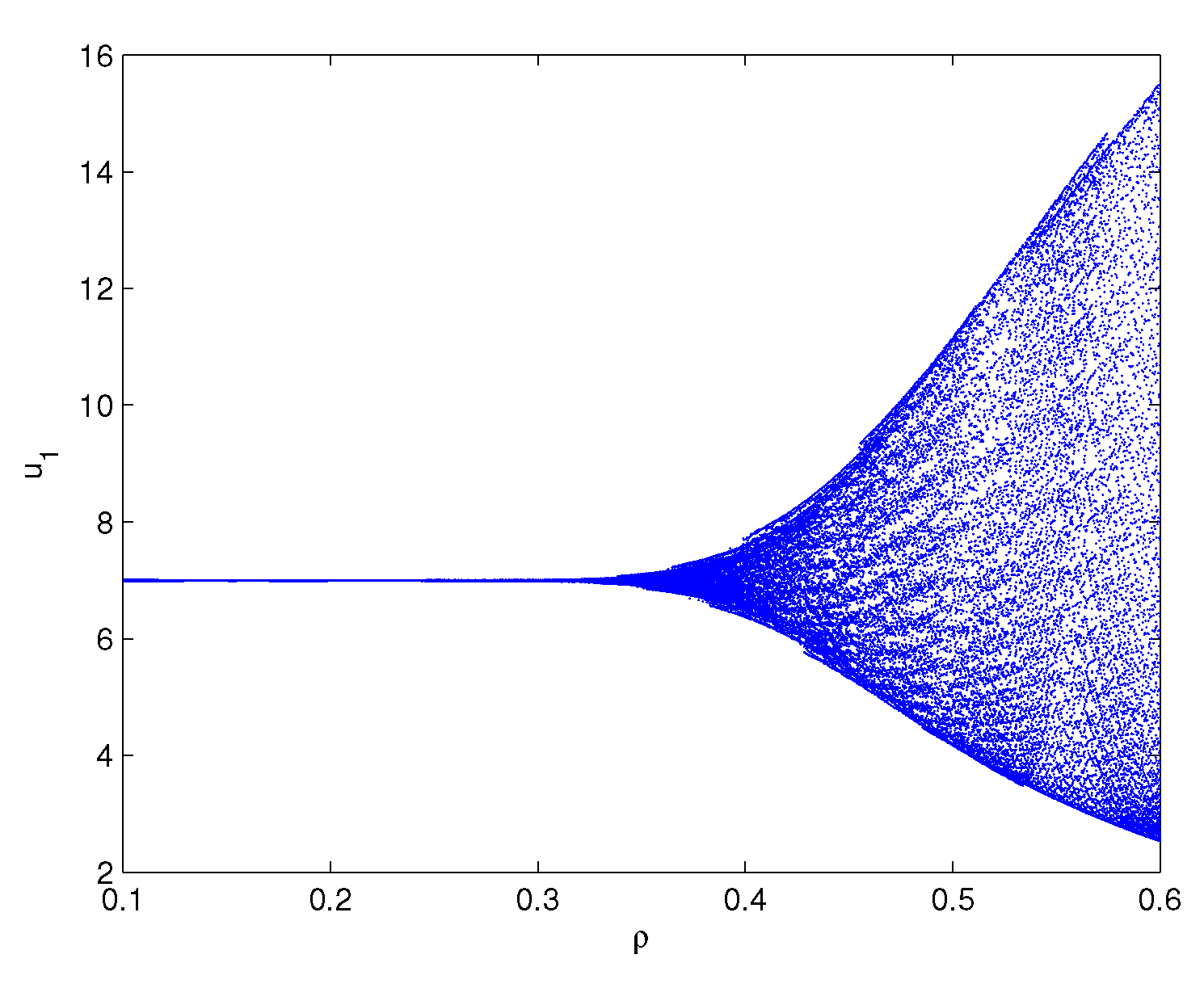
Figure 4.
Bifurcation diagram of model (6.1): x-axis represents the time delay and y-axis represents the variable . Model (6.1) admits the bifurcation value .
Figure 4.
Bifurcation diagram of model (6.1): x-axis represents the time delay and y-axis represents the variable . Model (6.1) admits the bifurcation value .
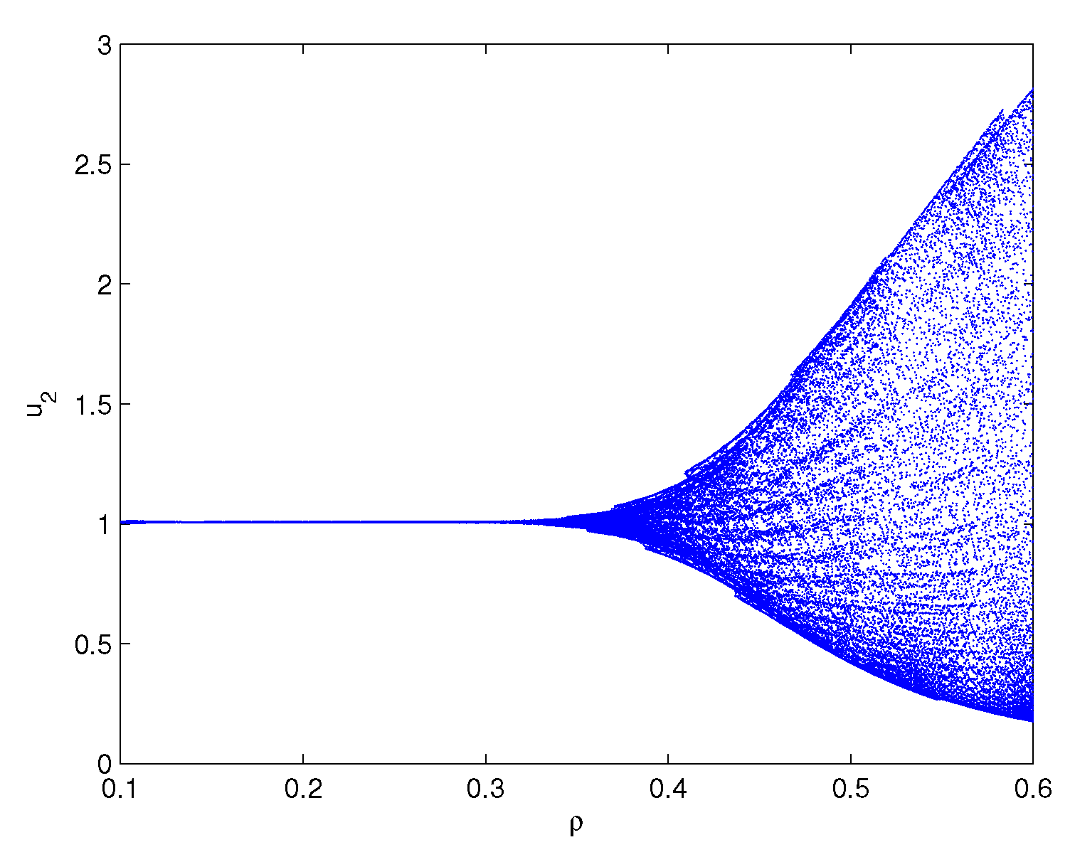
Figure 5.
Numerical experiment outcomes of system (6.2) involving the time delay The equilibrium point retains locally asymptotically stable condition.
Figure 5.
Numerical experiment outcomes of system (6.2) involving the time delay The equilibrium point retains locally asymptotically stable condition.
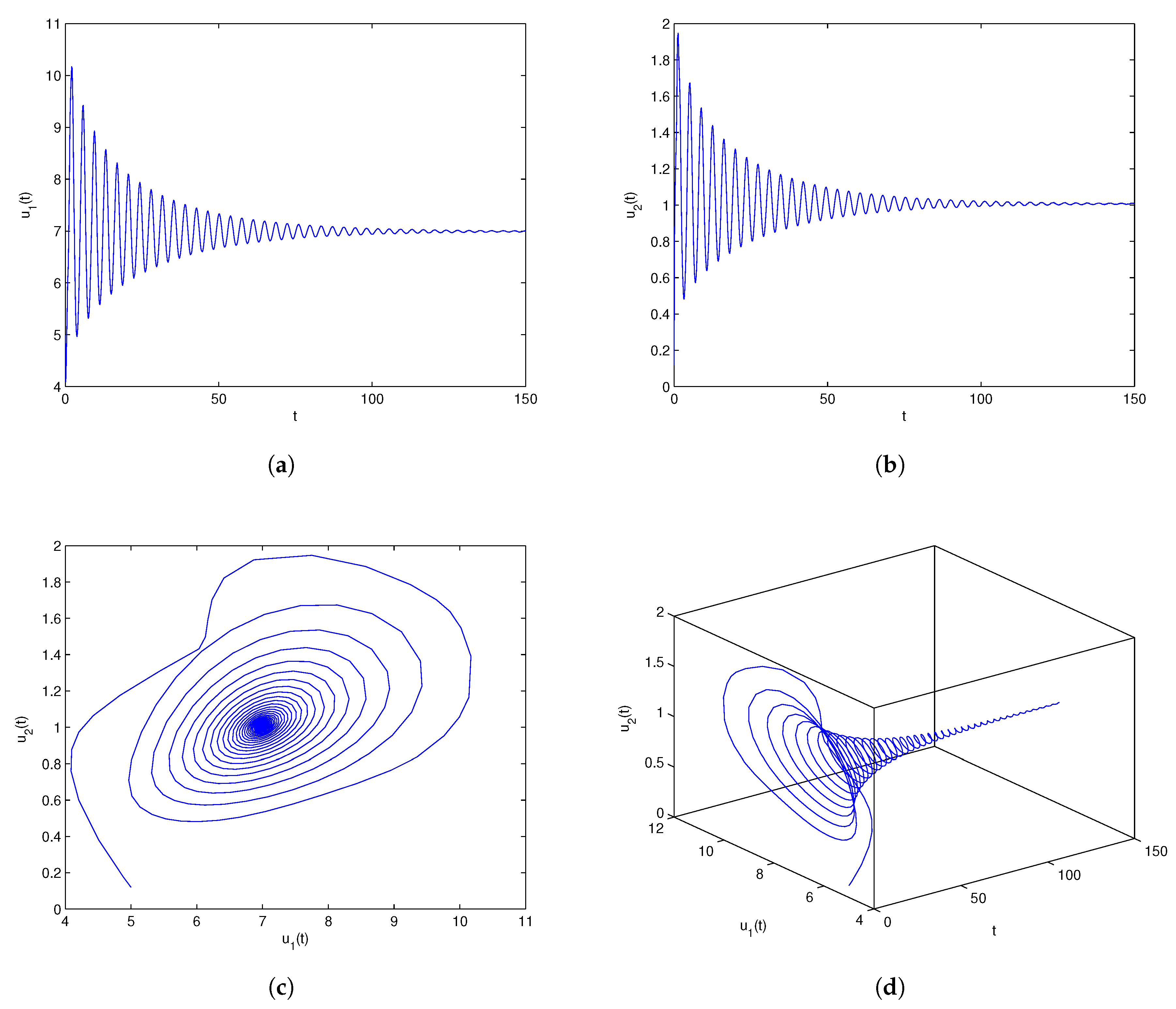
Figure 6.
Numerical experiment outcomes of model (6.2) involving the time delay A family of periodic solutions (namely, Hopf bifurcations) come into being in the nearby the equilibrium point .
Figure 6.
Numerical experiment outcomes of model (6.2) involving the time delay A family of periodic solutions (namely, Hopf bifurcations) come into being in the nearby the equilibrium point .
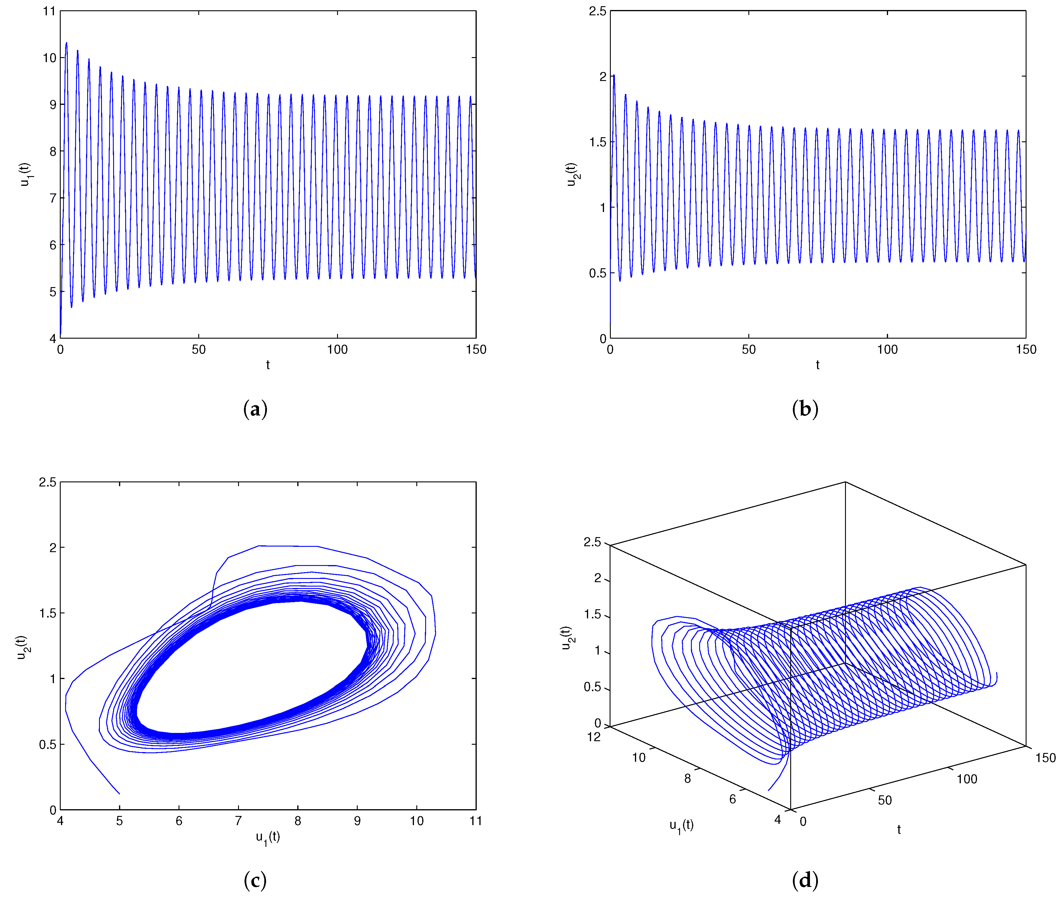
Figure 7.
Bifurcation diagram of model (6.2): x-axis represents the time delay and y-axis represents the variable . Model (6.2) admits the bifurcation value .
Figure 7.
Bifurcation diagram of model (6.2): x-axis represents the time delay and y-axis represents the variable . Model (6.2) admits the bifurcation value .
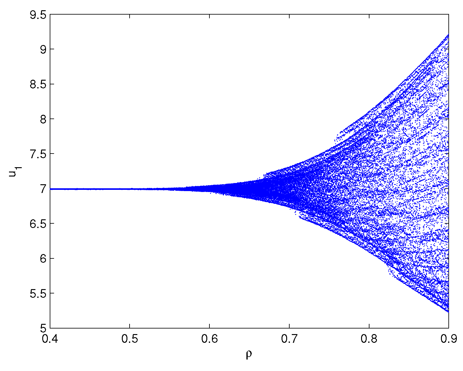
Figure 8.
Bifurcation diagram of model (6.2): x-axis represents the time delay and y-axis represents the variable . Model (6.2) admits the bifurcation value .
Figure 8.
Bifurcation diagram of model (6.2): x-axis represents the time delay and y-axis represents the variable . Model (6.2) admits the bifurcation value .
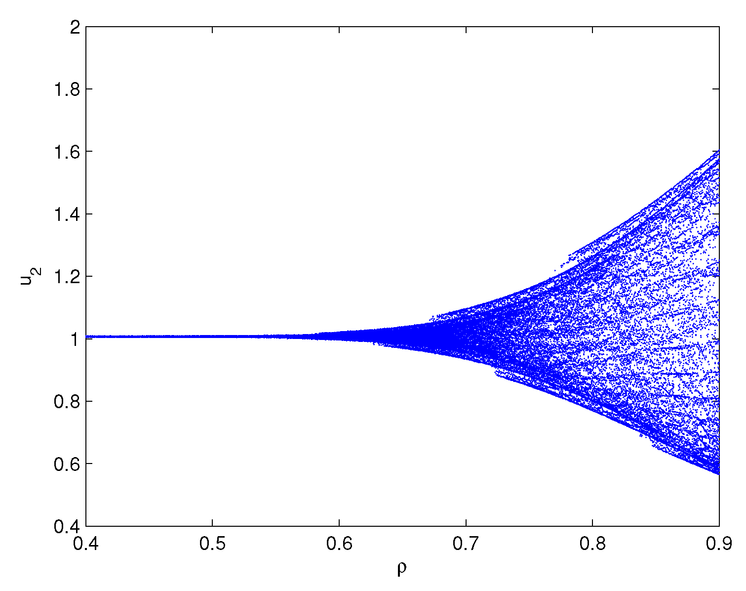
Figure 9.
Numerical experiment outcomes of system (6.3) involving the time delay The equilibrium point retains locally asymptotically stable condition.
Figure 9.
Numerical experiment outcomes of system (6.3) involving the time delay The equilibrium point retains locally asymptotically stable condition.
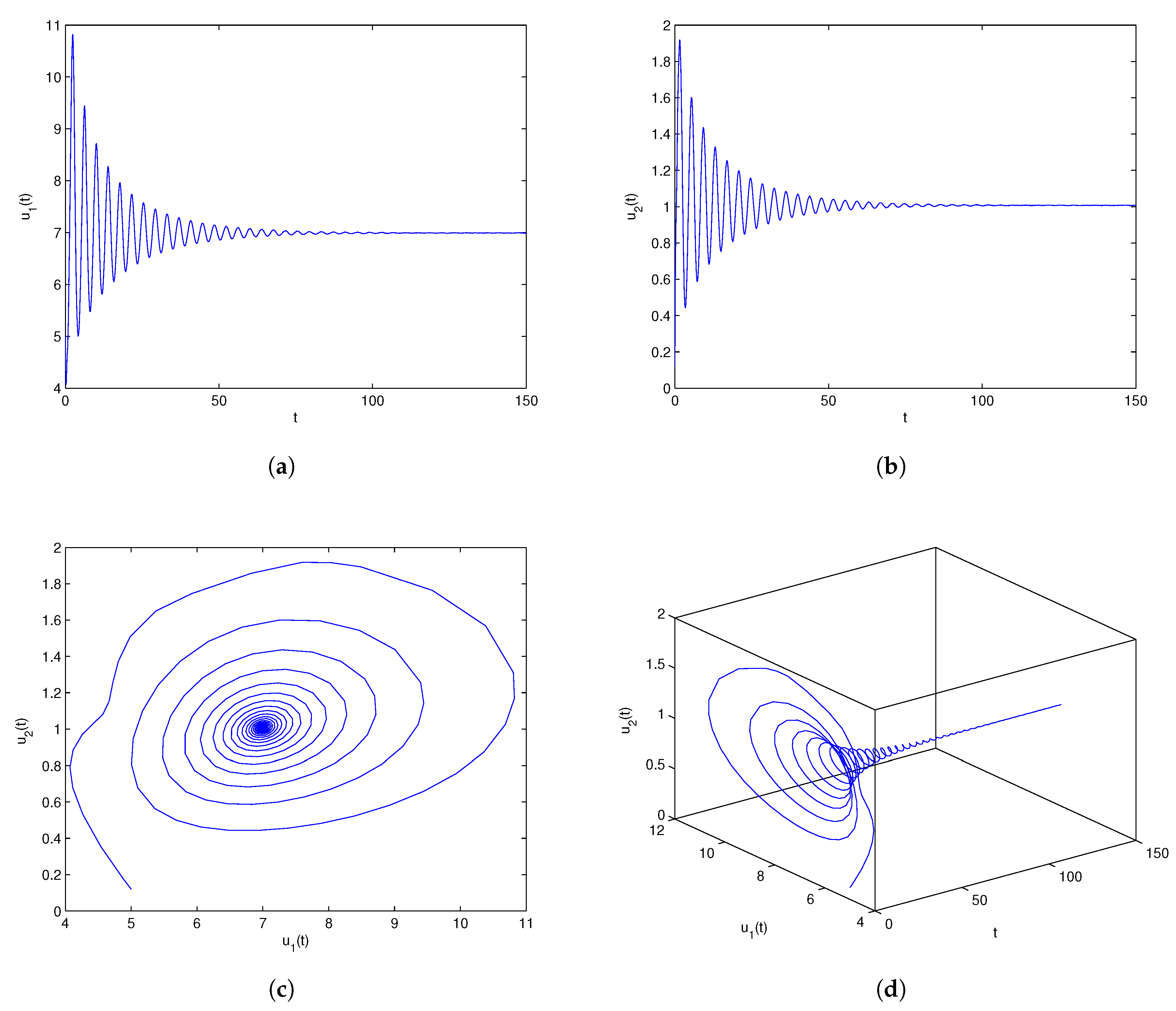
Figure 10.
Numerical experiment outcomes of model (6.3) involving the time delay A family of periodic solutions (namely, Hopf bifurcations) come into being in the nearby the equilibrium point .
Figure 10.
Numerical experiment outcomes of model (6.3) involving the time delay A family of periodic solutions (namely, Hopf bifurcations) come into being in the nearby the equilibrium point .
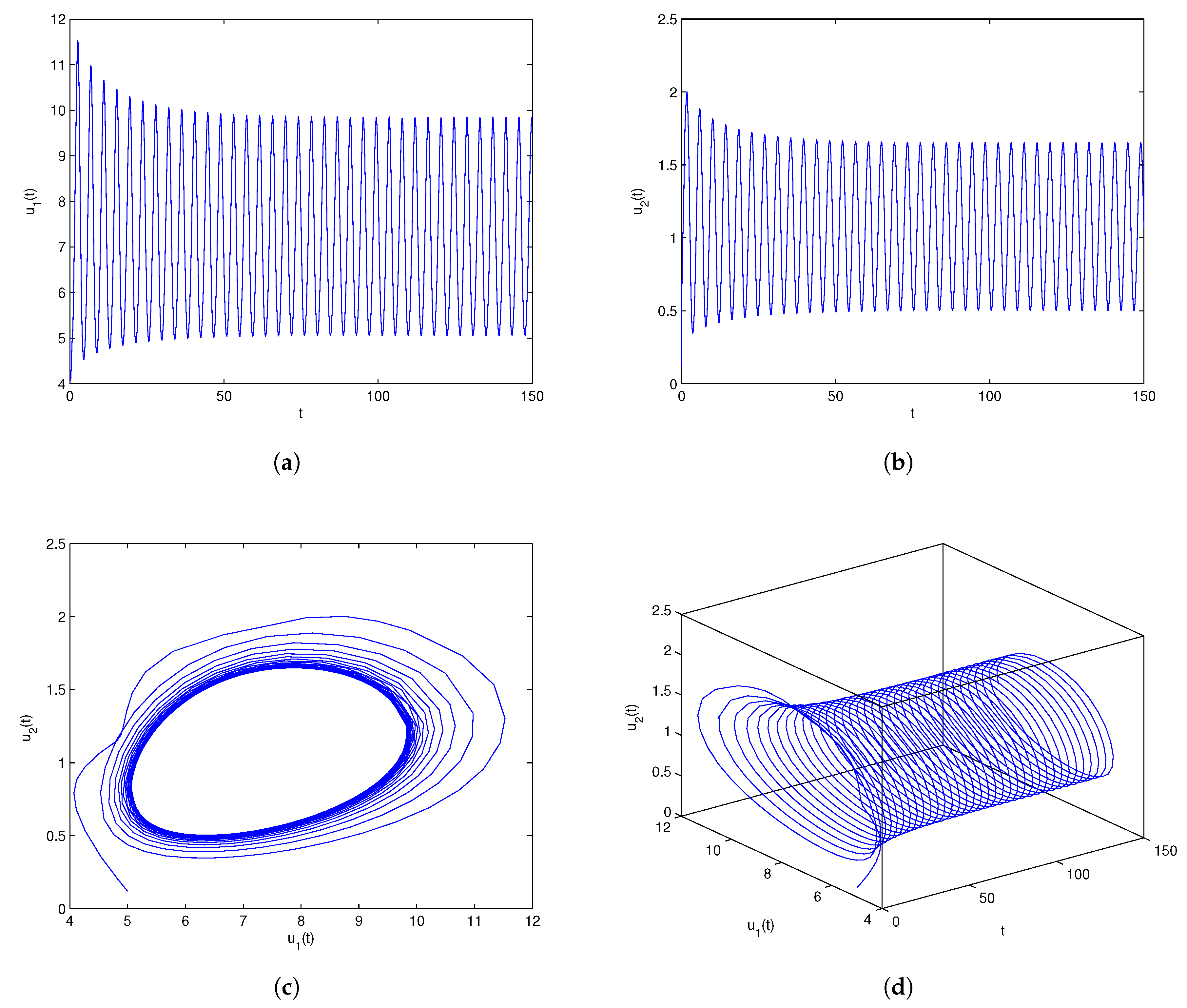
Figure 11.
Bifurcation diagram of model (6.3): x-axis represents the time delay and y-axis represents the variable . Model (6.3) admits the bifurcation value .
Figure 11.
Bifurcation diagram of model (6.3): x-axis represents the time delay and y-axis represents the variable . Model (6.3) admits the bifurcation value .
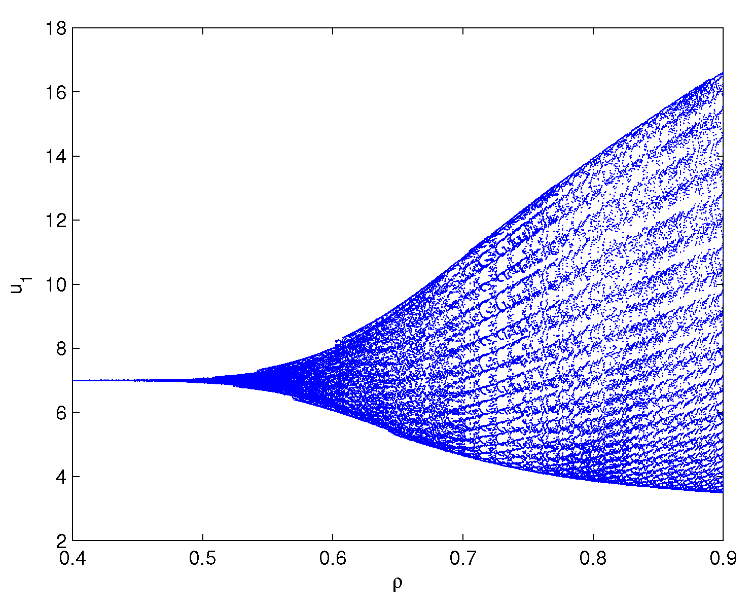
Figure 12.
Bifurcation diagram of model (6.3): x-axis represents the time delay and y-axis represents the variable . Model (6.3) admits the bifurcation value .
Figure 12.
Bifurcation diagram of model (6.3): x-axis represents the time delay and y-axis represents the variable . Model (6.3) admits the bifurcation value .
Disclaimer/Publisher’s Note: The statements, opinions and data contained in all publications are solely those of the individual author(s) and contributor(s) and not of MDPI and/or the editor(s). MDPI and/or the editor(s) disclaim responsibility for any injury to people or property resulting from any ideas, methods, instructions or products referred to in the content. |
© 2025 by the authors. Licensee MDPI, Basel, Switzerland. This article is an open access article distributed under the terms and conditions of the Creative Commons Attribution (CC BY) license (http://creativecommons.org/licenses/by/4.0/).
Copyright: This open access article is published under a Creative Commons CC BY 4.0 license, which permit the free download, distribution, and reuse, provided that the author and preprint are cited in any reuse.


