
Submitted:
20 January 2025
Posted:
21 January 2025
You are already at the latest version
Abstract
Fossil fuel depletion, environmental concerns, and energy efficiency initiatives drive the rapid growth in the adoption of electric vehicles. However, one of the significant challenges to the widespread deployment of this technology is the lengthy battery charging time. The concept of a battery swapping station has emerged as a solution to this issue, where depleted electric vehicle batteries are exchanged for fully charged ones in significantly less time. To this end, this paper evaluates the technical and economic performance of a grid-connected photovoltaic-wind hybrid power supply system for an electric vehicle battery swapping station. The objective is to investigate the viability of the hybrid power supply system as an alternative energy source by assessing its potential for cost savings and the overall cost-effectiveness of grid-connected systems for electric vehicle battery swapping stations. This is achieved through an optimal control model designed to minimize the total life cycle cost of the proposed system and reduce the consumption of electrical energy from the utility grid while maximizing system reliability, which is defined based on the loss of power supply probability. The optimal control problem is solved using mixed-integer linear programming, with decision variables including the power drawn from the utility grid, the number of wind turbines, and the number of solar photovoltaic panels. The effectiveness of this model is verified through a case study. Simulation results demonstrate the desirable performance of the proposed system, with the optimal number of wind turbines and solar photovoltaic panels determined to be 64 and 420, respectively. The total life cycle cost of the installation, in South African Rand, is estimated at R 1,963,520.12, leading to energy cost savings of up to 41.58% for the studied case. Additionally, an economic analysis, conducted through life cycle cost analysis, includes the initial capital investment as well as the maintenance and operation costs over the system’s lifetime. The LCC analysis results indicate a payback period of 5 years and 6 months, demonstrating that the proposed system is both economically and technically feasible.
Keywords:
electric vehicle battery swapping station
; grid-connected hybrid renewable power supply systems
; multi-objective optimisation
; mixed integer linear programming
; life cycle cost analysis
1. Introduction
The growing concerns about climate change, combined with the need to reduce reliance on fossil fuels and the imperative to mitigate environmental impacts related to energy, have spurred global efforts toward transitioning to sustainable energy sources [1,2]. The energy consumption forecast for years to come only strengthens this trend, especially in light of demographic trends and development in many countries around the world [3]. This is highly critical for countries listed as developed countries where the stakes are high in balancing economic growth with environmental sustainability [2,3]. For instance, in South Africa, the energy sector grapples with multiple challenges, including supply constraints, frequent power outages (load shedding), rising electricity costs, and environmental degradation [4,5]. The current power grid cannot meet the load demand, meaning an additional burden such as charging the depleted electric vehicles (EVs) battery could be harmful [6,7,8]. As part of South Africa’s commitment to sustainable development and energy security, there is a growing emphasis on diversifying the energy mix and promoting the integration of renewable energy.
The electric vehicle (EV) market has grown exponentially in the past decade. The International Energy Agency (IEA) predicts that the global EV market could reach 55–72 million units by 2025, representing approximately 8% of all vehicle sales [9]. The adoption of EVs could reduce fossil fuel consumption, subsequently decreasing the amount of greenhouse gases (GHGs) and other pollutants released into the atmosphere during road travel. Besides reducing fossil fuel dependence, EVs emit considerably less compared to internal combustion engines (ICEs) [10,11]. With the widespread adoption of EVs, the demand for EV charging infrastructure is inevitably increasing. Thus, the success of EV market is closely tied to the availability, efficiency, and accessibility of charging systems. However, several barriers still hinder the broader adoption of EVs, such as the high cost of EV battery replacement, the limited driving range, and long charging times. Despite the increasing number of EV charging stations, charging times often remain excessively long. This situation necessitates using fast charging methods, which can negatively impact the longevity of EV batteries. A promising solution to these challenges is the implementation of EV battery swapping stations (BSSs). BSSs offer a more convenient and efficient way to recharge EV batteries by allowing drivers to exchange their depleted EV batteries for fully charged ones within minutes. These stations charge the EV batteries according to a predetermined strategy before making them available for the next swap, effectively alleviating concerns about energy availability and long charging times. BSSs can also charge the depleted EV batteries ahead of time, especially during off-peak hours, to meet peak swapping demands, which is potentially compatible with the peak demand of the power supply system. The depleted EV batteries being charged can be integrated into the energy management system, where their charging is scheduled or discharged to supply power to the utility grid. This charging solution is imminent to offer seamless mobility since swapping a depleted EV battery takes less time than charging it. Moreover, BSSs can be considered as a demand response resource that benefits both the environment and the power supply system. BSSs play a crucial role in supporting EV adoption and reducing carbon emissions from transportation. Nevertheless, integrating BSSs with the existing power utility grid remains a significant challenge due to the high operating costs associated with generation and maintenance [12,13,14,15,16,17,18]. These challenges can be mitigated by integrating the BSS with renewable energy source systems (RES), thereby enhancing the stability of the power utility grid.
In light of the growing interest in BSSs, many companies globally are engaging in pilot installations to develop and implement BSS technology for the EV industry, showing that battery swapping technology is a promising and cost-effective alternative to traditional plug-in charging method [19,20,21,22]. Significant research studies have also focused on developing and optimizing BSSs by integrating them with RES. These research studies have often investigated different methods to improve the planning and operation of BSSs, highlighting their potential benefits over traditional plug-in charging methods. Rao et al. proposed an optimization charging model based on a questionnaire experiment to investigate and optimize the battery-swapping behaviours of EV users. The authors discovered that optimizing EV user behaviour in BSS can lead to improved energy efficiency [23]. Xu et al. concentrated on the mechanism of the smart battery charging and swapping operation service network for EVs, including their general design and operational mode. Two distinct types of demonstration installation projects were given, each of which elaborated on the state of EV infrastructure building. Finally, a performance study of the charging behaviours of electric taxis in fast charging stations based on queuing theory was provided. The simulation results revealed that the service duration and the number of generators affected on the average waiting time and queue length [24]. Yan et al. provided a real-time energy management strategy for a BSS-based smart community microgrid (SCMG) that uses fluctuating renewable energy to charge EV batteries and traditional household loads. A novel Lyapunov optimization framework based on queuing theory was developed to solve the suggested model. The proposed method reduces complicated energy scheduling to a single optimization problem, making it suitable for real-time applications. According to simulation studies, BSS employed for dual purposes might increase overall system economics and enable the incorporation of renewable energy compared to standalone operations [25]. Mahoor et al. concentrated on developing a mathematical model for uncertainty constrained in BSSs for the optimal operation that covered both random customer demand of fully charged batteries and leveraged the available batteries for minimising operation costs through demand shifting and reselling energy. The authors solved the BSS scheduling problem for one station using mixed integer linear programming and predicted battery depletion by presenting a feasible solution. Simulation approaches were also utilised to show the proposed model’s effectiveness and assess its practicality in reaching the lowest possible operating cost [26]. In [27], Liu et al. achieved optimal BSCS operation by proposing a closed-loop supply chain-based BSCS model to realise the combined operation of battery charging stations and battery swap stations. In contrast, a network calculus-based service model was used to ensure the quality of battery swapping service at BSS. The simulation results confirmed the practicality of the suggested model and the heuristic solution, which had small optimal losses and required less computing time. Yang et al. suggested a dynamic operating model of a BSS in the electricity market. The novel mathematical programming model tries to find the optimal short-term battery strategy, with 24-hour simulation results demonstrating the methodology’s practicality and practicability [28]. Zheng et al. developed a battery swap station operation model for a fleet of electric buses in public transportation. An optimal solution was found by examining the parameters of the electric city buses and battery leasing mode in order to minimise the charging impact on the grid while maximising the yearly profit of the battery swap station [29]. Based on life cycle cost (LCC) minimization, Zheng et al. provided a methodology for the optimal design of battery charging/swap stations in distribution networks. According to the findings, battery swap stations are more suited for public transportation in distribution networks [30]. Wu et al. developed an optimal charging strategy to increase PV-generated power self-consumption and service availability while accounting for forecast mistakes. After introducing the basic structure and operation model of PV-based BSS, they offered three indices to measure operational performance. Then, for each time slot, the PSO algorithm was designed to compute the optimal charging power and minimise the charging cost. The proposed charging strategy reduces the influence of expected uncertainty on the battery swapping service’s availability. Finally, a case study was used to simulate a day-ahead operating plan, a real-time decision-making method, and the proposed PSO charging technique for PV-based BSS. The simulation results showed that the suggested technique might significantly enhance the self-consumption of PV-generated electricity while minimising charging costs [31]. Tan et al. developed a model that included an open-loop queue of electric vehicles and a closed-loop queue of batteries. The first research stream provided queuing network models as a framework for modelling and building BSSs with a local charging mode. They experimented on a single battery swap station and used modelling approaches to give valuable information for the infrastructure development of real battery swapping services [32]. In [33], Wu et al. presented an optimization model for a BSS to minimize costs by determining the optimal charging schedule for swapped EV batteries. Three factors were considered: the number of batteries taken from stock to handle all swapping orders from incoming EVs, the possibility of charging damage from high-rate chargers, and the electricity cost for different times of the day. A series of simulation studies are executed to assess the feasibility of the proposed model and compare the performance between the proposed algorithm and typical evolutionary algorithms. The proposed model can determine the optimal charging schedule according to the results. Additionally, the proposed algorithm performed significantly better than the other optimization algorithms [33].
Previous research has focused on optimizing BSS by exploring various strategies and approaches to improve efficiency, such as optimal location and sizing of stations, dynamic scheduling and dispatching of EV batteries, and incorporating renewable energy to reduce carbon footprint and operational costs. However, these studies often lack a comprehensive analysis of the technical and economic viability of integrating renewable energy sources like solar and wind power and the development of smart grid technologies to enhance the overall performance and sustainability of battery swapping networks within grid-connected hybrid renewable power supply systems.
To the best of the authors’ knowledge, no research has yet examined the grid-connected hybrid renewable power supply system for EV BSS from the perspective of South Africa. This gap in the literature motivated the current study. The rapid increase in EV adoption, influenced by new vehicle brands, infrastructure development, and government initiatives aimed at reducing transport sector emissions by 5% by 2050, underscores the need for cleaner mobility solutions in South Africa [34,35,36]. Despite the growing network of public charging stations across the country, inadequate charging infrastructure remains a significant barrier to widespread EV adoption [36,37]. Effective BSS design and operation must address complex factors, including the intermittent nature of renewable energy, EV battery charging patterns, EV battery swapping demand, and utility grid stability. This paper investigates the technical and economic factors influencing BSS performance and their integration with the utility grid, thereby filling the gap. Understanding these aspects is essential for maximizing benefits and ensuring the sustainability of EV BSS.
This paper assesses the techno-economic feasibility and optimal design of a grid-connected hybrid renewable power generation system to support EV BSS in South Africa. A multi-objective optimization model is developed to minimize the total life cycle cost of the proposed system and the electricity cost purchased from the utility grid through optimal power flow control within the demand-side management framework while maximizing the reliability of the grid-connected wind-solar system, expressed by the loss of power supply probability (LPSP). This developed multi-objective optimization model can provide the EV BSS with a continuous power supply at a low cost, and the scheduling strategy can be implemented for the swapping EV battery so that the swapping demand must be satisfied at any given time of the day. Designing such a system to effectively minimize costs and power purchases from the utility grid while meeting reliability requirements is challenging. Therefore, mixed integer linear programming (MILP) is employed for the multi-objective optimal sizing, offering advantages over heuristic algorithms due to the quick solvability of linear programming (LP) sub-problems and the guarantee of obtaining the global optimum through a convex feasible region [38].
The remaining sections of this paper are organized as follows: Section 2 describes the mathematical model formulation of the proposed system, including technical and economic parameters. Section 3 presents a case study reflecting real-world conditions. Section 4 discusses the simulation results of the case study. Finally, conclusions are drawn in Section 5.
2. Mathematical Model Formulation
2.1. Schematic Model Layout
The schematic layout of the proposed grid-connected wind-photovoltaic hybrid power generation system for the EV BSS is shown in Figure 1. The main components of the proposed system are the vertical wind turbines (WT), the photovoltaic generator (PV), the inverters, and the battery swapping station (BSS), which comprises the charging apparatus and swapping service for the depleted EV batteries. For such a proposed system, the size of the hybrid renewable power generation system depends on the charging and swapping demand service at the BSS. The BSS uses three distinct sources of electrical energy to charge EV batteries. These sources include the electricity generated by vertical wind turbines, the electricity generated by the photovoltaic generator, and the electricity obtained from the utility grid. To ensure that the demand for swapping depleted EV batteries is met efficiently, it is crucial to accurately determine the properties of power sources utilized to charge the depleted EV batteries. By doing so, the charging process can be optimized to effectively replenish the EV batteries and meet the needs of the drivers. The depleted EV batteries are charged with the utmost priority using clean and renewable electricity generated by the vertical wind turbine and solar photovoltaic panel. However, this charging process is dependent on the availability of adequate resources. In other words, if the electricity generated by the vertical wind turbine and solar photovoltaic panel is insufficient, then the electricity from the utility grid is used to charge the depleted EV batteries. This ensures that the depleted EV batteries are charged optimally and that the use of electricity from the utility grid is minimized. Suppose the electricity generated by the vertical wind turbine and the solar photovoltaic panel is more than the charging demand of the depleted EV batteries. In that case, the surplus electricity generated can be sold to the utility grid. The fluctuating electricity prices at different times of the day significantly impact the charging process’s overall cost. Effectively managing this impact is achieved through implementing a time-of-use (TOU) tariff, a critical factor in determining the power source for recharging depleted EV batteries. The TOU tariff is strategically designed to incentivize power consumption during off-peak hours when electricity prices are lower. This approach serves the dual purpose of minimizing stress on the utility grid during peak hours and optimizing the cost-effectiveness of the charging process. Depending on the prevailing TOU tariffs, the BSS can be supplied by either hybrid power generation or the utility grid. This flexibility ensures that the BSS draws power from the utility grid during periods of lower electricity prices, contributing to cost savings. By doing so, the power flow from the utility grid is managed efficiently and cost-effectively, maintaining reliability and stability. This strategic utilization of the TOU tariff and power source selection not only minimizes operational costs but also contributes to the overall sustainability and resilience of the EV charging infrastructure. The decision to charge the depleted EV batteries is determined by multiple factors, such as the power flow’s limitations and the TOU electricity tariff within the utility grid. The power flow’s limitations depend on the available power capacity and the current power demand in the system. The TOU tariff considers the cost of electricity at different times of the day, where charging the depleted EV batteries during off-peak hours can be more cost-effective. On the other hand, the decision to replace the depleted EV batteries with fully charged ones is determined by the EV driver’s arrival or the swapping service demand at the BSS. The BSS can offer a convenient solution for EV drivers who want to continue their journey without waiting for their EV battery to charge. In this paper, the electrical energy generated by the hybrid renewable power generation system is deliberately not reintegrated into the utility grid.
2.2. Sub-Models of the Proposed System Components
The following sections provide comprehensive descriptions and mathematical models of the various components of the proposed system.
2.2.1. Wind Turbine System
In wind energy systems, the air is moved to generate power through its kinetic energy. Wind energy is a resource that has the potential to be abundant, and that might be easily harvested and converted into useful energy using standard technology. In addition to allowing for the efficient use of distributed resources, wind energy systems promise to make energy supply systems more flexible, robust, secure, stable, and profitable [39]. As a result, it is crucial to have a reliable assessment of the resources available at a wind farm to generate electricity there. In general, when the wind speed varies between the "cut-in wind speed" () and the "rated wind speed" , the total amount of energy generated by the wind turbine is proportional to the cube of the wind speed. The model used to determine the wind turbine’s output power is displayed in Figure 2. The wind turbine cannot generate electricity when the wind speed is less than the cut-in speed. When the wind speed exceeds the cut-in speed, the power generated by the wind turbine rises by the cube of the wind speed until it reaches its maximum value at the rated speed. It is known as the rated power , and it is the power for which the wind turbine is designed. As shown in Figure 2, the wind speed is very high at some given time, which is dangerous for wind turbines. This is referred to as "cut-out wind speed" . The wind turbine operation must stop at this point because it has reached the . Equation 1 represents a description of the simplest straightforward model of this behaviour to simulate the output power of the wind turbine [40]:
where, denotes the wind speed at sampling time t, denotes the rated wind speed, denotes the cut-in wind speed, denotes the cut-out wind speed, and denotes the rated power of the wind generator.
If all the wind speeds and rated power are known, Equation 1 can be used to determine the wind turbine’s power output. Therefore, the rated power of the wind turbine generator can be expressed as
where and are the gearboxes and generator efficiency, respectively, denotes the density of air , denotes the power coefficient of the wind turbine, which is the ratio of the power output of the wind generator divided by maximum power, denotes the sweeping area of the turbine rotor . In contrast, denotes the rated wind speed .
To maximise the amount of energy available from the wind turbine system, the wind profile may need to be adjusted based on the height of the wind turbine. The wind speed vertical profiles may be simulated using two mathematical models, such as the logarithm and power law. As a common method of analysis in research, power laws will be applied to this research study [41]. When using this model, the wind speed at the hub height is
where denotes the wind speed measured at the reference height (), V denotes the wind speed measured at the hub height (h), and denotes the coefficient of ground surface friction, which has a value of more than 0.25 in forested areas and less than 0.1 in flat or watery areas [41].
Multiple wind turbines can be coupled in parallel to meet the proposed system requirements. One of the design variables is the number of wind turbines () when operating in parallel. The wind turbine size is among the variables that influence the output power of the wind turbine. When is taken into account as the number of wind turbines, the output power generated by the wind turbine at sampling time is calculated from
Depending on the operation conditions, the net power supply of the wind turbine to the power system is limited by boundaries, which can vary between zero and the maximum output power generated. This can be expressed as
where 0 is the minimum capacity of the output power generated by the wind turbine, and is the maximum capacity of the output power generated by the wind turbine.
Furthermore, the limited availability number of wind turbines is constrained so that
where is the minimum number of wind turbines taken as zero and is the maximum number of wind turbines that can fit into the allocated area as given by
where is the total sweeping area available for the wind turbine at the EV BSS, and is the sweeping area of the wind turbine rotor.
2.2.2. Solar Photovoltaic System
As the name suggests, the principle of the electricity generated by the photovoltaic is related to photons and voltage. By definition, photovoltaic is a technology that converts the radiant (photon) energy from sunlight into DC power [42]. A photovoltaic cell is a crucial element in converting light energy directly into electricity through a chemical and physical process called the photovoltaic effect. The term describes a device whose electrical properties change when exposed to light, such as voltage, current, or resistance. Solar photovoltaic panels, also known as solar photovoltaic modules, comprise solar photovoltaic cells. A solar photovoltaic module or solar photovoltaic panel comprises several solar photovoltaic cells arranged in an integrated group, all facing the same direction. In contrast, an array or solar photovoltaic array comprises the solar photovoltaic module or solar photovoltaic panel connected in series, parallel, or a combination of the two [43]. The size of the photovoltaic panel, its efficiency, solar radiation, and the surrounding temperature all affect how much electricity the photovoltaic system can generate. The output power generated by a solar photovoltaic array is given by [43]:
where is the power output generated by the PV array, is the area of the PV array exposed to solar radiation, is the solar radiation that reaches the PV array, and is the energy conversion efficiency of the PV generator.
It is possible to express the solar irradiation according to the time during the day using
where, is a geometric factor used to indicate the ratio between plane-tilted beams’ irradiation incident and plane-horizontal beams’ standard irradiation, is the diffuse irradiation, and is the hourly global irradiation.
The ambient temperature and hourly isolation impact the solar PV generator energy conversion efficiency . It can be stated that
where denotes the temperature factor for PV generator efficiency, which ranges from 0.004 to 0.006 per oC, denotes the reference cell temperature, denotes the efficiency of power conditioning, denotes the cell temperature, and denotes the manufacturer-rated efficiency of the solar array module. The cell temperature is
where is the nominal cell operating temperature, while is the ambient temperature.
The output generated power of a PV array varies with the number of PV panels () installed. The variables, such as the size of the panels used and other factors, affect the total output power generated by the PV system. When is taken into account as the number of solar photovoltaic panels, the total output power generated by the PV panels at sampling time is calculated from
Depending on the operation conditions, the net power supply of the solar photovoltaic panels to the power system is determined by sizing and optimal positioning, and it can vary between zero and the maximum output power generated. This can be stated in the following way:
where 0 and represent the minimum and maximum capacity of the solar PV panel, respectively.
Furthermore, the limited availability number of solar PV arrays is constrained so that
where is the minimum number of solar PV panels taken as zero and is the maximum number of solar PV panels that can fit into the allocated area as given by
where denotes the total available surface area for the solar PV panel at the EV BSS, and denotes the area of the PV array that is exposed to solar radiation.
2.2.3. Inverter
The inverter is a very important device in grid-connected renewable energy systems. It is used to synchronize the output power and set the output voltage. Inverters convert DC power sources to AC power and vice versa. The output power of the wind turbine is in AC electricity, which is transformed into DC by the inverter for later use. The charging demand is in AC power form, and the output power from the solar PV system, which is in DC electricity, is converted again by the inverter to AC electricity. The inverters provide other features to ensure the protection and monitoring of power instability for the entire system. Therefore, it is essential to have high inverter efficiency. The inverter efficiency is given by [44]:
where is the efficiency of the inverter, is the power out from the inverter, is the power which enters into the inverter. In order to ensure safe operation and efficiency, the inverter’s rated power should often be oversized by 10% to 30% [45]. Therefore, the inverter-rated power is
where is the oversized coefficient of the inverter. The inverter lifetime is less than the installation lifespan. The number of times during the lifetime of the installation that the inverter is required to be replaced is expressed by:
where is the lifespan of the installation project, while is the lifespan of the inverter.
2.2.4. Utility Grid Power Supply System
The current utility grid was not designed to meet the demand to charge the depleted EV battery [46]. In contrast to household loads, the full charge of the depleted EV batteries requires high power levels and substantial amounts of energy [47,48]. When charging the depleted EV batteries can have a significant impact on voltages, component loads, and losses depending on the supplied loads and the design of the utility grid. The impacts on the utility grid are significantly influenced by the charging power and penetration level of the EVs. The number of EV batteries as a percentage of all EVs at the BSS is the general definition of the penetration level. The power from the utility grid is modelled as an all-time available power source charging the depleted EV batteries at the BSS. The energy drawn from the utility grid is given by
where is the power flow from the utility grid to charge the depleted EV batteries at the BSS, and is the sampling time.
Therefore, the energy cost that can be extracted from the utility grid is determined by the local electricity market policy and time of use (TOU) tariff. Two parameters are required for utility grid modelling: the maximum amount of electricity that can be drawn from the utility grid in kW (the maximum grid demand) and the price of electricity purchased from the utility grid in ZAR/kWh (the power price). The energy cost that can be drawn from the utility grid when charging the depleted EV batteries can be calculated from
where is the TOU electricity price at the t-th sampling interval per . Additionally, the power flow from the utility grid can be constrained to a limited range using:
2.2.5. Battery Swapping Station Power Demand Mathematical Modelling
An EV BSS is a facility designed for EV owners to efficiently exchange their depleted EV batteries for fully charged ones within a few minutes. This innovative concept has emerged as a potential solution to address the challenges associated with traditional plug-in charging methods for EVs [21,22]. A standard EV BSS has one or more battery swapping units, enabling multiple EVs to exchange their depleted EV batteries simultaneously. The power demand of a BSS is typically influenced by various factors, including the process of charging and swapping the depleted EV battery, as well as the characteristics of the EV battery itself. These characteristics encompass parameters such as EV battery capacity, EV battery technology, and the depleted EV battery’s state of charge (SoC) before charging [49]. Proper modelling of power demand is essential at the BSS, particularly during the charging period of depleted EV batteries, in order to meet the swapping demand when the EVs arrive. Equations (22) and (23) respectively represent the total charged power and total discharged power of depleted EV batteries at the BSS. These equations calculate the cumulative power by summing the power contributions or power outputs of all depleted EV batteries present at the BSS [50].
where n is the total number of the depleted EV batteries at the BSS, is the total charging power of the depleted EV batteries at the BSS, is the total discharging power of the depleted EV batteries at the BSS, is the charging power of one depleted EV battery at the BSS, is the discharging power of one depleted EV battery at the BSS. Each depleted EV battery undergoes a charging or discharging process similar to a conventional battery. The charging of these depleted EV batteries is determined based on their State of Charge (SoC) during specific time intervals, which quantifies the available capacity relative to the maximum capacity achievable when the EV battery is fully charged. Taking these factors into account, the SoC of every EV battery at sampling interval inside the BSS can be generally expressed by [26,50]:
where is the duration of time interval in minute, is the efficiency of one EV battery (%) and it given by Equation (25).
During the battery swapping process, a fully charged EV battery is swapped for a depleted EV battery from an arriving EV at the BSS. This swap period prevents the EV battery from being charged or discharged as the swapping operation progresses. Consequently, during this swapping time period, the power and SoC of the EV battery are set to zero, as described by Equation (26).
Before the battery swapping period, the depleted EV battery must be fully charged in preparation for the next swap. Therefore, the energy management system must ensure that a sufficient number of fully charged EV batteries are available at each time interval to accommodate the upcoming swaps. This requirement is articulated in Equation (27).
The total power demand at the BSS is based on the power capacity of the charging station. The discretized charging power demand for each depleted EV battery is added together to determine the overall charging power demand. In other words, the total expected power demand for all n depleted EV batteries charged at the BSS at time t can be estimated using the following Equation (28).
where is the total expected power demand of all depleted EV batteries charged at time , and n is the total number of the depleted EV batteries at the BSS.
2.3. Technical and Economic Parameters of the Proposed System
Before applying the optimisation design, it is necessary to define technical and economic parameters to systematically define the proposed system’s total cost and reliability. The total life cycle cost parameter and the loss of power load probability (LPSP) parameter are employed in this paper to quantify the overall cost and to measure the reliability of the proposed system, respectively. These two parameters are explained in the following:
2.3.1. Economic Evaluation Parameters of the Proposed System
The economic evaluation indicators are mathematical methods that are used to compare the cost and benefits of the installations regarding the economic, commercial, and social aspects, and it has a significant impact on the optimization design of a grid-connected renewable energy system [51,52]. This paper considers the economic parameter based on the life cycle cost (LCC) concept as the economic criterion to evaluate the installation financial viability. When using the LCC method, all future cash flows are discounted to present value cash flows by considering the time value of money and installation lifespan. In other words, the LCC covers all the cash inflows and outflows into the proposed system in its entire lifetime [53,54]. It compares initial investment options and identifies the least cost alternatives for a x period (years). The costs included in the LCC evaluation are the initial capital investment (), operation and maintenance cost (), replacement cost (), and salvage cost (). Mathematically, the LCC is given by [55,56]:
The initial capital investment cost is the amount of money required to set up all components in the proposed system, which includes the cost of purchasing materials, civil work, and the installation of each component. Meanwhile, the operating and maintenance cost present value indicates the maintenance costs incurred throughout the proposed system’s lifespan for all components to ensure proper operation. This represents the total of all yearly planned operation and maintenance costs. The operator’s wage, inspections, insurance, and any necessary planned maintenance are all included in the operation and maintenance cost. A general form to express the present value of the operation and maintenance cost of a hybrid system is [57,58]:
where is the operation and maintenance cost in the first year, r is the inflation rate, i is the interest rate, and is the lifespan of the installation. The replacement cost is a cautionary expense over the lifetime of the proposed system for replacing any components. During the lifespan of the proposed system, some components, like the inverter, could need to be changed. Again, the price of these components is liable to change in the future. The present value of the replacement cost may be calculated by taking into account the real interest rate (i) and the inflation rate () of the component to be replaced [57,58]. It can be expressed as
where is the capital cost of the component per , is the nominal capacity of the replacement system component in , is the inflation rate of the component replaced taken equal to r, y is the index of the components, is the lifetime of the components, is the number of replacement of each component over the system lifespan period of the installation . And finally, the cost incurred at the end of the system’s lifespan is known as the salvage cost. This includes the cost of removal and disposal and the proposed system’s salvage value.
In order to assess the economic viability of the hybrid system, it is necessary to calculate its overall life cycle cost. This entails totalling the LCCs of each component so that:
where is the life cycle cost of the wind turbine, is the life cycle cost of the photovoltaic generator, and is the life cycle cost of all the inverters.
- a)
- LCC of the wind turbine system
The initial capital investment cost of the wind turbine system includes the cost of purchasing and installing the wind turbine at the BSS. The purchase cost of the wind turbine may vary depending on its size, efficiency, and brand. In addition, installation costs can vary depending on factors such as the location and complexity of the installation process. Overall, the initial capital investment cost of the wind turbine system can be estimated by factoring in the cost of purchasing and installing the wind turbine, as shown in (33).
where is the initial capital investment cost of the wind turbine generator system, is the initial cost of the wind turbine, and is the installation cost of the wind turbine. Assuming that the installation cost is considered to be 20% of the initial cost of the wind turbine generator [59,60]. Then, the initial capital investment cost of the wind turbine generator system is given by:
where is the capital cost of the wind turbine generator per , is the total number of the wind turbine generator, and is the power rating of the wind turbine generator. It is assumed that the operation and maintenance cost of the wind turbine generation system will be 5% of its initial capital investment cost [59,60]. Considering the annual cost of wind turbine generator increasing at the inflation rate (r), the net present value of the operation and maintenance cost of the wind turbine generator () can be calculated using
with,
Assuming that the installation lifespan and the wind turbine generator lifetime are equal, the replacement cost of the wind turbine generator is zero (). The salvage cost is neglected. As a result, by using (34) and (35), the LCC of the wind power generation system can be obtained from
- b)
- LCC of the photovoltaic system
The initial capital investment cost of the PV system includes the purchase and installation costs of the solar panel at the BSS. The purchase cost of the solar panel may vary depending on its size, efficiency, and brand. Additionally, installation costs may vary based on factors such as the location and complexity of the installation process. Overall, the initial capital investment cost of solar PV system can be estimated by factoring in the cost of purchasing and installing the solar panel, as shown in (37).
where is the initial capital investment cost of the solar PV system, is the initial cost of the solar panel, and is the installation cost of the solar panel. Some research studies have suggested that the installation cost of a solar PV panel is a significant factor that accounts for 40% of the total initial cost [59,60]. By considering the installation costs along with other associated expenses, the initial capital investment cost of the solar PV panel system is given by:
where is the capital cost of the solar PV panel per , is the total number of solar PV panels, is the power rating of the solar PV, is the output power generated by the solar PV panel at each instant t. Solar PV panels’ operation and maintenance cost is assumed to be 1% of its initial capital investment cost [59,60]. Considering the annual cost of solar PV panels increasing at the inflation rate (r), the net present value of the operation and maintenance cost () can be calculated from
with
If it is assumed that the installation and the solar PV panels have the same lifetime, then the replacement cost of the solar PV panel is zero (). The salvage cost is ignored. By using equations (38) and (39), the overall LCC of the PV power generation system () is given by:
- c)
- LCC of the inverters
The initial capital investment cost of the inverter includes all the expenses incurred in the purchase and installation of the inverter at the BSS. This includes the cost of the inverter unit, as well as any additional equipment, parts, and labour required to complete the installation. The initial capital investment cost is given by
where is the initial capital investment cost of the inverter, is the initial cost of the inverter, and is the installation cost of the inverter. This paper doesn’t take into account the installation cost of the inverters. Then, the initial capital investment cost can be calculated from
where is the capital cost of the inverter per , is the oversize coefficient of the inverter, and is the efficiency of the inverter. The inverter lifespan () is less than the installation lifespan. Additional investment is required before the end of the installation project. Then, the net present value of the replacement cost of the inverter is given by
where .
In this paper, the operation and maintenance cost of the inverter, as well as its salvage cost, have not been taken into account. The LCC of the inverter (), in general terms, is given by
2.3.2. Reliability Consideration of the Proposed System
In this paper, the reliability of the proposed system is evaluated by the loss of power supply probability (LPSP). LPSP is a statistical parameter which indicates a failure of distributed power systems to meet the charging demand [61]. The reliability of grid-connected renewable energy systems is sized and evaluated using the LPSP approach as one of the technology-implemented criteria. For a given period N, the LPSP is defined as the ratio of all the loss of power supply (LPS) values for that period N to the sum of the charging demand. Due to the proximity of the substation and the installation area for the proposed system to the EV BSS, wiring losses within the distribution network are assumed to be insignificant. The LPSP is given by [62,63]:
where is the loss of power supply at sampling time , and is the hourly load demand of the charging demand of depleted EV batteries at the BSS.
Assuming that the LPSP is a value between 0 and 1, the charging demand at the BSS is never fulfilled when the LPSP is equal to 1. On the other hand, the charging demand is always satisfied when the LPSP is equal to 0. Therefore, the LPS is given by
where is the power flow from the utility grid charging the depleted EV batteries at the BSS, is the power flow from the solar PV system charging the depleted EV batteries at the BSS, and is the power flow from the wind turbine charging the depleted EV batteries at the BSS.
2.4. Optimisation Problem Formulation and Proposed Algorithm
This section presents the MILP formulation of the proposed optimisation model for the grid-connected hybrid wind-solar power system designed for the EV BSS. The model determines the optimal sizing combination and management strategy under the considered TOU electricity tariff, with the aim of minimizing the overall life cycle cost and the charging cost of the depleted EV batteries from the utility grid while maximizing its reliability. By integrating both wind and solar energy sources, the model leverages renewable energy to reduce dependency on the utility grid. However, the inherent variability and intermittency of wind and solar power introduce challenges in maintaining a consistent energy supply.
2.4.1. Objective Function
The objective of the optimisation model is to minimize the total life cycle cost () of the proposed system and the electricity cost purchased from the utility grid () to charge the depleted EV batteries at the BSS through optimal power flow control within the demand-side management framework while maximizing its reliability. The objective function is given in (47), in which the first part represents the total LCC, and the second part is the cost of the energy consumption from the utility grid.
where is a weighting factor. The weighting factor is employed to convert the multi-objective optimization problem to a single-objective optimization problem for the EV BSS, which should generate one optimal solution. In this paper, the priority of the total LCC and the cost of the energy consumption from the utility grid are treated as equally important and are assumed to be balanced. Thus, the weighting factor is 0.5. The decision variables are the hourly power from the utility grid , the number of wind turbine , and the number of solar PV panels which both depend on the total surface area and for the wind turbine and solar photovoltaic panel respectively available at the EV BSS. The hourly power from the utility grid is a continuous variable, while the number of WT and solar PV panels must be an integer value. Taking into account these decision variables, the objective function (47) can therefore be rewritten as
where denotes the capital cost of the photovoltaic generator per , denotes the number of the solar photovoltaic panel, denotes the output power generated by the photovoltaic panel at sampling time t, denotes the power rating of a photovoltaic generator, denotes the capital cost of the wind turbine generator per , denotes the number of the wind turbine, denotes the output power generated by the wind turbine at sampling time t, denotes the power rating of a wind turbine, denotes the capital cost of the inverter per , denotes the efficient of the inverter, denotes the oversize coefficient of the inverter, N the sampling period, denotes the power from the grid, is the sampling time, is the weighting factor.
2.4.2. System Constraints
As a result of power supply generation and charging demand at the EV BSS, the objective function has some operational, technical, and reliability constraints. These constraints are mathematically represented as follows:
▸Reliability: To maximize the reliability of the proposed system, the LPSP is subject to the following constraints:
▸The power flow limits: For safety reasons, all the power flows connected to various components should be kept within the manufacturer’s requirements. Therefore, at any sampling time t, the power flows can be within a specific limited range of zero to their rated power, and these can be represented as follows:
▸Wind turbine numbers: The limited number of wind turbines is bounded by the maximum and minimum units of wind turbines considered. The economic constraints define the upper limit, while the configuration considered determines the lower limit. This means
▸Solar photovoltaic panel numbers: The limited number of solar PV panels is bounded by the maximum and minimum units of solar PV panels considered. The economic constraints define the upper limit, while the configuration considered determines the lower limit:
2.4.3. Algorithm for Solving the Optimisation Problem
The optimization problem formulated in this paper is a mixed-integer linear programming problem (MILP). Since the number of wind turbines and PV panels must be an integer and, at the same time, the power flow from the utility grid must be a continuous value, the optimization problem is solved using the SCIP (Solving Constraint Integer Programs) solver in the Matlab OPTI Toolbox 1. The algorithm for solving a MILP problem using the SCIP solver involves several key steps. Initially, SCIP reads and parses the problem, converting it into an internal representation. This is followed by preprocessing, where SCIP simplifies the problem by removing redundant constraints and variables, tightening bounds, and detecting infeasible sub-problems. The core of the algorithm is the branch-and-bound method, which iteratively divides the problem into smaller sub-problems by branching on fractional variables. At each node of the branch-and-bound tree, SCIP uses linear programming (LP) relaxations to obtain bounds and employs cutting planes to improve these bounds. Additionally, heuristics are applied to find feasible solutions quickly, and primal and dual bounds are updated to guide the search process. SCIP also integrates constraint propagation techniques to further reduce the search space. The process continues until all sub-problems are either solved or pruned, resulting in the optimal solution to the MILP problem [38,64]. A scalarization technique is necessary to solve multi-objective optimization problems using MILP. This technique employs weight factors to convert multiple objective functions into a single aggregated objective function [65,66]. Therefore, the objective function and constraints can be formulated using the canonical form:
subject to:
where represents the objective function, x is the vector containing the decision variables representing the optimal number of wind turbines and solar panels, as well as the cost of the energy purchased from the utility grid, A and b are the coefficients associated with inequality constraints, and are the lower and upper bounds of the decision variables.
3. General Data
A case study is conducted utilizing real-world data from an operational BSS network to validate the feasibility and effectiveness of the proposed system, as illustrated in Figure 1. These data provide reliable and practical input parameters for the analysis and simulations, making them ideal for addressing this multi-optimization problem. Renewable energy sources demonstrate the applicability and benefits of the developed model. The charging demand at the EV BSS is met using a combination of vertical wind turbines, solar PV panels, and the utility grid. This paper doesn’t feed the energy generated into the utility grid. The subsequent sections present the daily load profile of the EV BSS power demand, followed by an introduction to the necessary input data used in the model for simulating hybrid renewable power output and the time-of-use (TOU) electricity tariff for the selected location.
3.1. EV BSS Power Demand Load Profile
To accurately assess the energy requirements of the EV BSS, a detailed load profile was constructed using historical data from an operational BSS. The chosen EV BSS is a heavy-duty truck swapping station situated at a central logistics hub in Shanghai Port, China, where energy consumption patterns reflect the high and variable demand associated with commercial EV operations. The data was recorded over a representative period, capturing daily and seasonal demand variation. Figure 3 illustrates the daily energy consumption at the EV BSS, highlighting peak demand periods that coincide with high traffic volumes and operational hours. The load profile serves as the basis for sizing the hybrid renewable energy system and determining the optimal mix of energy sources.
3.2. Renewable Energy Power Supply
The proposed hybrid renewable power generation system incorporates wind turbines and solar PV panels as primary energy sources, supplemented by grid electricity to ensure a reliable supply. The input parameters for WT system power generation, such as the wind speed, and for solar PV power generation, such as the solar radiation and ambient temperature, are obtained from a typical day in the low-demand season in Cape Town, South Africa, as referenced in [67]. Figure 4 presents the hourly average wind speed at 10 m above the ground. The wind speed varies throughout the day, with a daily average of 2.46 m/s. The windiest period occurs between 2:00 and 3:00 PM, with an average wind speed of 4.6 m/s, while the calmest period is observed between 1:00 and 2:00 AM, with an average wind speed of 1.08 m/s. For more information, the average hourly wind speed over the year is presented in Figure 5. Additionally, the daily average for PV generation is depicted in Figure 6, indicating that the peak incident short-wave radiation for solar PV power generation reaching the ground’s surface over a wide area is approximately 0.42 around 12:45 PM. For more information, the annual short-wave radiation for solar PV power generation reaching the ground’s surface over a wide area is presented in Figure 7, which gives significant seasonal variation with the peak brighter and lowest darker period of the year around December and June, respectively. The hybrid power system is designed to ensure that the EV BSS power demand is met at any given time, particularly when electricity from the utility grid is expensive. The sizing of the wind and PV system is tied to the initial equipment cost and available capital, directly impacting power generation and reducing energy costs from the utility grid.
3.3. Time-of-Use Electricity Tariff
The South African power grid is managed by the national utility, "Eskom", with electricity tariffs regulated by the National Energy Regulator of South Africa (Nersa). Eskom’s tariff structure typically includes both flat and dynamic TOU pricing systems. TOU pricing is a demand-side management strategy that reflects the varying costs of electricity production throughout the day and is divided into three periods: off-peak (), standard-peak (), and on-peak (). These periods correspond to times when electricity demand and generation costs are low, moderate, and high, respectively. In the context of the optimization problem, the TOU electricity tariff significantly influences the energy efficiency of the EV BSS. This paper considers the Eskom Megaflex TOU tariff scheme, which applies to urban and industrial consumers who both consume energy from the utility grid and generate energy at the same point of supply. For this case study, the 2023/2024 Eskom Megaflex electricity tariff for high-demand season (from June to August) weekdays is used as the basis for the TOU electricity tariff analysis given as 2:
with is the South African currency (Rand), and t represents the time of day in hours.
4. Simulation Results and Discussion
This section presents the simulation results obtained from the optimization model described in the previous section. The simulation results regarding the system’s performance, cost-effectiveness, and reliability are analysed. Additionally, the impact of varying key input parameters, such as the number of wind turbines, PV panels, and TOU electricity tariffs, is also discussed. The outcomes provide insights into the optimal design and management strategies for a grid-connected wind-solar hybrid power generation system for the EV BSS. Furthermore, a comprehensive economic analysis is conducted by assessing the payback period and cost-effectiveness of installing the proposed system.
4.1. Optimal Hybrid Power System Sizing and Management Strategy
The optimization problem is a MILP. Since the number of WTs and solar PV panels must be integers, and the power flow from the utility grid must be continuous, the optimization problem is solved using the SCIP solver in MATLAB’s OPTI Toolbox over a 24-hour horizon with a sampling interval of . The technical and economic input parameters used for the simulation based on the case study and the developed optimization problem in this paper are listed in Table 1. The simulation is conducted for a specific day with the lowest monthly average wind speed and shortwave solar power, as shown in Figure 5 and Figure 7, respectively. The objective is to determine the most efficient and optimal design for the hybrid system, focusing on optimal sizing of the WT and solar PV systems to ensure energy autonomy and cost efficiency for the EV BSS. In the optimization process, the objective function’s weighting factor balances the energy sources’ cost and reliability. The number of WTs and solar PV panels is determined to meet the charging demand at the EV BSS while minimizing reliance on grid electricity, thereby reducing operational costs. Figure 8 represents the power generated by hybrid power generation. The power generated by the WT system is provided according to Equation 1, and the power generated by the solar PV system is provided according to the radiation from Figure 6. When the weighting factor is set to 0.5, the simulation results indicate that the optimal configuration for the hybrid power generation systems consists of 64 wind turbines and 402 solar PV panels, with a total LCC of ZAR 1,963,520.12. The results remain consistent for any weighting factor value within the range of 0.27 to 0.71. Varying the weighting factor between 0 and 0.27 prioritizes the hybrid power generation systems over the utility grid, potentially leading to excess energy being absorbed by the utility grid. Conversely, setting the weighting factor between 0.71 and 1 prioritizes the utility grid, resulting in all charging power being supplied solely by the power flow from the utility grid, with the hybrid power generation systems becoming oversized. Figure 9 shows the simulation results of the charging demand along with the optimal output power flows from each source over a 24-hour period. It can be seen that the charging demand varies throughout the 24 hours, with peak demand occurring around 9 AM, 2 PM, and 7 PM. Hybrid power generation systems provide a significant proportion of the power needed to meet the charging demand, substantially reducing the utility grid operation cost. From 00:00 to 06:00, the power generated by the hybrid power generation systems is very low due to minimal wind speeds and the unavailability of solar PV. At this period, the charging demand is met by power from the utility grid. As wind speeds increase, the power generated by the WTs also increases, and the charging demand is met by the utility grid and the WTs system. From 06:00 to 09:00, the solar PV system begins to generate power, which, along with the WTs, is prioritized to meet the charging demand. The utility grid supplements any power deficit. From 09:00 to 17:00 and 17:00 to 19:00, the hybrid power generation systems generate sufficient energy to meet the charging demand, with the utility grid serving as a backup to supply any remaining deficit power. From 19:00 to 22:00 and 22:00 to 00:00, the charging demand is met by the power from the utility grid and WTs, which have lower wind speeds resulting in a lower power supply, but at this same time the solar PV is not available. In general, hybrid power generation systems produce more power during the day than at night. Applying Eskom’s TOU electricity tariff to the proposed system results in an electricity cost of R7 676.39 for the charging demand shown in Figure 3. Incorporating the optimization model reduces this cost to ZAR 4 483.53, representing a cost saving of ZAR 3 192.85, which is 41,6 % of the daily cost savings. Table 2 and Table 3 summarize the simulation results, showing the number of WTs, PV panels, the total LCC, and cost savings achieved through optimal control intervention. These results are based on the average daily cost in the case study, with the daily cost annualized to reflect an average yearly amount. The results demonstrate the feasibility and effectiveness of integrating wind and solar energy to power the EV BSS, offering a sustainable and resilient solution for EV charging and swapping infrastructure.
4.2. LCC Analysis for the Payback Period
Economic feasibility is assessed through a cost-benefit analysis of cash outflows and inflows associated with installing the proposed system. The installation feasibility can be evaluated using various methods, considering both environmental benefits and economic indicators [68,69,70]. The LCC method accounts for the time value of money and installation lifespan by discounting all future cash flows to their present value. The comparative advantage of LCC is that it covers all the cash inflows and outflows into the system in its lifetime. Therefore, the discounted present value (DPV) of one cash flow occurring in a future period ( year) can be represented as:
where represents the discounted present value (discounted cash flow) of the future cash flow, is the nominal value of a cash flow amount in a future period ( year), r is the discount rate, and z is the time in years before the future cash flow occurs. In this LCC analysis, the discount rate reflects the time value of money or the cost of tying up capital and may also allow for the risk that the payment may not be received in full. The actual discount rate is given by the difference between the average interest and inflation rate. The interest rate represents the opportunity value of time; that is, the compensation should be paid to defer additional expenditure in the current year until a later year, while the inflation rate is the percentage increase or decrease in prices during a specified period and usually over a month or a year. The percentage tells you how quickly prices rose during the period. The interest rate is an essential parameter in the LCC analysis of an installation project, and thus, the unit cost of generation is an essential parameter. The average interest 3 and inflation rate 4 in this paper is 8.25% and 4.6%, respectively, indicating the time value of the money in South Africa as of July 2024. The component prices are based on South African market rates. In this LCC economic analysis of energy efficiency projects, both operational and maintenance costs, as well as cost savings, are considered. Once FV (z) is determined, the net present value (cumulative cash flow) is calculated as follows [70]:
where NPV is the net present value (cumulative cash flow), CC is the total investment capital cost of the project. Subsequently, the discounted payback period (PBP) can be determined using the following equation [70]:
where denotes the last year with a negative NPV. Table 4 provides the approximate prices of the various components of the proposed grid-connected wind-photovoltaic hybrid power supply system, leading to the total investment capital cost (CC).
Some assumptions are made while carrying out LCC analysis of the proposed system. The annual operation and maintenance costs are assumed to increase proportionally throughout the installation service lifetime, along with the annual optimal cost-benefit. The annual cost-benefit represents the amount the EV BSS owner would have spent each year without implementing the proposed system. Table 5 presents the LCC analysis of the proposed system under the optimal control strategy, with the salvage cost neglected for the payback period (PBP). From Table 5, the estimated total investment capital cost is a negative cash flow in the financial statement represented in brackets as (5 691 216.10). The cash flows and PBP are calculated following the assumptions that the annual optimal cost benefits and annual operational and maintenance costs will proportionately increase throughout the lifetime of the proposed system. The cumulative cash flows continue to decrease in negative cash flow until it crosses to positive cash flows. The payback/break even happens at the point when the cumulative cash flow equals zero. This is the point at which all the invested capital is recovered. For the proposed system, the PBP occurs after 5 years and 6 months. Thereafter, the cumulative cash flow goes into positive values, meaning the total investment capital cost has been fully recovered, and all the revenue in subsequent years follows is pure benefit or profit. If an installation lifetime is 20 years and PBP of around 5 years and 6 months, the EV BSS owner can recover his total capital investment within a reasonable time and will have more than 10 years to generate profit, which is guaranteed.
5. Conclusions
This paper presents a novel techno-economic evaluation and optimal design approach for a grid-connected wind-photovoltaic hybrid power supply system tailored for electric vehicle battery swapping stations. The proposed optimization model, developed using mixed-integer linear programming, aims to minimize the total life cycle cost and the cost of electrical energy consumption from the utility grid while maximizing system reliability. The decision variables considered include the number of wind turbines, solar photovoltaic panels, and power drawn from the grid. For the case study, the results demonstrate that the implementation of energy cost management under a time-of-use (TOU) electricity tariff yields substantial savings, reducing electricity costs from the grid by 41.58%. The optimal solution consists of 64 wind turbines and 420 solar photovoltaic panels, resulting in a total life cycle cost of 1,963,520.12 ZAR. A cost-effectiveness analysis performed using LCC as the economic performance indicator reveals a payback period of 5 years and 6 months, highlighting the financial benefits of the proposed hybrid system. Furthermore, this optimization approach not only significantly reduces energy costs but also ensures high system reliability. This techno-economic feasibility and design optimisation offers an adaptable solution for various applications. The developed method can be extended to different locations, proving its flexibility in optimizing grid-connected wind-photovoltaic hybrid power systems, especially in areas where energy storage costs may be prohibitive. The proposed system offers a cost-effective and reliable solution for electric vehicle battery swapping stations, with promising potential for widespread implementation in South Africa’s roadways, driving both economic and environmental benefits.
Author Contributions
Conceptualization, L.T.-E.N. and D.D.; methodology, L.T.-E.N. and D.D.; software, L.T.-E.N.; validation, L.T.-E.N., D.D., L.M. and S.W.; formal analysis, L.T.-E.N. and D.D.; investigation, L.T.-E.N., D.D., L.M. and S.W.; resources, L.T.-E.N., S.W.; data curation, L.T.-E.N., S.W.; writing—original draft preparation, L.T.-E.N.; writing—review and editing, L.T.-E.N., D.D., L.M. and S.W.; visualization, L.T.-E.N.; supervision, D.D. and L.M.; project administration, L.T.-E.N. and D.D.; funding acquisition, L.T.-E.N. All authors have read and agreed to the published version of the manuscript.
Funding
This research received no external funding.
Conflicts of Interest
The authors declare no conflict of interest.
References
- Skovgaard, J. EU climate policy after the crisis. Environmental Politics 2014, 23(1), 1–17. [Google Scholar] [CrossRef]
- McCarthy, J. A socioecological fix to capitalist crisis and climate change? The possibilities and limits of renewable energy. Environment and Planning A: Economy and Space 2015, 47, 2485–2502. [Google Scholar] [CrossRef]
- Eder, L.; Provornaya, I. Analysis of energy intensity trend as a tool for long-term forecasting of energy consumption. Energy Effciency 2018, 11(8), 1971–1997. [Google Scholar] [CrossRef]
- Kenny, A. The rise and fall of Eskom and how to fix it now. Policy Bulletin South African Institute Race Relations (IRR) 2015, 2(18), 1–22. [Google Scholar]
- Giglmayr, S.; Brent, A.C.; Gauch´e, P.; Fechner, H. Utility-scale PV power and energy supply outlook for South Africa in 2015. Renewable Energy 2015, 83, 779–785. [Google Scholar] [CrossRef]
- Khan, W.; Ahmad, F.; Alam, M.S. Fast EV charging station integration with grid ensuring optimal and quality power exchange. Engineering Science and Technology, an International Journal 2019, 22, 143–152. [Google Scholar] [CrossRef]
- Asaad, M.; Ahmad, F.; Alam, M.S.; Rafat, Y. Iot enabled monitoring of an optimized electric vehicles battery system. Mobile Networks and Applications 2018, 23(4), 994–1005. [Google Scholar] [CrossRef]
- Shaikh, F.; Alam, M.S.; Asghar, M.; Ahmad, F. Blackout mitigation of voltage stability constrained transmission corridors through controlled series resistors. Recent Advances in Electrical & Electronic Engineering (Formerly Recent Patents on Electrical & Electronic Engineering) 2018, 11, 4–14. [Google Scholar]
- International Energy Agency. Global EV Outlook 2021. Available online: https://www.iea.org/reports/global-ev-outlook-2021.
- Alexander, M.; Tonachel, L. Projected greenhouse gas emissions for plug-in electric vehicles. World Electric Vehicle Journal 2016, 8(4), 987–995. [Google Scholar] [CrossRef]
- Sujitha, N.; Krithiga, S. Res based ev battery charging system: A review. Renewable and Sustainable Energy Reviews 2017, 75, 978–988. [Google Scholar] [CrossRef]
- Alanazi, F. Electric Vehicles: Benefits, Challenges, and Potential Solutions for Widespread Adaptation. Applied Sciences 2023, 13(10), 6016. [Google Scholar] [CrossRef]
- Zhan, W.; Wang, Z.; Zhang, L.; Liu, P.; Cui, D.; Dorrell, D.G. A review of siting, sizing, optimal scheduling, and cost-benefit analysis for battery swapping stations. Energy 2022, 124723. [Google Scholar] [CrossRef]
- Dharmakeerthi, C.; Mithulananthan, N.; Saha, T. Impact of electric vehicle fast charging on power system voltage stability. International Journal of Electrical Power& Energy Systems 2014, 57, 241–249. [Google Scholar]
- Nyamayoka, L.T.; Masisi, L.M.; Dorrell, D.G.; Wang, S. Optimisation Design of On-Grid Hybrid Power Supply System for Electric Vehicle Battery Swapping Station. In 2023 IEEE International Future Energy Electronics Conference (IFEEC) 2023, 296-299. IEEE.
- Fan, Y.; Guo, C.; Hou, P.; Tang, Z.; et al. Impact of electric vehicle charging on power load based on tou price. Energy Power Eng 2013, 5, 1347–1351. [Google Scholar] [CrossRef]
- Sehar, F.; Pipattanasomporn, M.; Rahman, S. Demand management to mitigate impacts of plug-in electric vehicle fast charge in buildings with renewables. Energy 2017, 120, 642–651. [Google Scholar] [CrossRef]
- Amiri, S.S.; Jadid, S.; Saboori, H. Multi-objective optimum charging management of electric vehicles through battery swapping stations. Energy. 2018, 15(165), 549–562. [Google Scholar] [CrossRef]
- Adu-Gyamfi, G.; Song, H.; Nketiah, E.; Obuobi, B.; Adjei, M.; Cudjoe, D. Determinants of adoption intention of battery swap technology for electric vehicles. Energy 2022, 15(251), 123862. [Google Scholar] [CrossRef]
- Danilovic, M.; Liu, J.L.; Müllern, T.; Nåbo, A. Almestrand Linné, P. Exploring battery-swapping for electric vehicles in China 1.0.
- Chen, X; Xing, K; Ni, F; Wu. Y; Xia, Y. An electric vehicle battery-swapping system: Concept, architectures, and implementations. IEEE Intelligent Transportation Systems Magazine 2021, 14, 175–194.
- Lebrouhi, B.E.; Khattari, Y.; Lamrani, B.; Maaroufi, M.; Zeraouli, Y.; Kousksou, T. Key challenges for a large-scale development of battery electric vehicles: A comprehensive review. Journal of Energy Storage 2021, 44, 103273. [Google Scholar] [CrossRef]
- Rao, R; Zhang, X; Xie, J; Ju, L. Optimizing electric vehicle users’ charging behavior in battery swapping mode. Applied Energy 2015, 155, 547–559. [CrossRef]
- Xu, X; Yao, L; Zeng, P; Liu, Y; Cai, T. Architecture and performance analysis of a smart battery charging and swapping operation service network for electric vehicles in china. Journal of Modern Power Systems and Clean Energy 2015, 3(2), 259–268. [CrossRef]
- Yan, J; Menghwar, M; Asghar, E; Panjwani, M.K; Liu, Y. Real-time energy management for a smart-community microgrid with battery swapping and renewables. Applied Energy 2019, 238, 180–194. [CrossRef]
- Mahoor, M; Hosseini, Z.S; Khodaei, A. Least-cost operation of a battery swapping station with random customer requestsests. Energy 2019, 172, 913–921. [CrossRef]
- Liu, X; Zhao, T; Yao, S; Soh, C.B; Wang, P. Distributed operation management of battery swapping-charging systems. IEEE Transactions on Smart Grid 2018, 10, 5320–5333.
- Yang, S; Yao, J; Kang, T; Zhu, X. Dynamic operation model of the battery swapping station for ev (electric vehicle) in electricity market. Energy 2014, 65, 544–549. [CrossRef]
- Zheng, D; Wen, F; Huang, J. Optimal planning of battery swap stations. International Conference on Sustainable Power Generation and Supply (SUPERGEN 2012) 2012, 2012, 153.
- Zheng, Y; Dong, Z.Y; Xu, Y; Meng, K; Zhao, J.H; Qiu, J. Electric vehicle battery charging/swap stations in distribution systems: comparison study and optimal planning. IEEE transactions on Power Systems 2013, 29, 221–229.
- Wu, S; Xu, Q; Li, Q; Yuan, X; Chen, B. An optimal charging strategy for pv based battery swapping stations in a dc distribution system. International Journal of Photoenergy 2017, 2017.
- Tan, X; Sun, B; Tsang, D.H. Queueing network models for electric vehicle charging station with battery swapping. in 2014 IEEE International Conference on Smart Grid Communications (SmartGridComm) 2014, 1–6.
- Wu, H; Pang, G. K. H; Choy, K. L; Lam, H.Y. An optimization model for electric vehicle battery charging at a battery swapping station. IEEE Transactions on Vehicular Technology 2017, 67(2), 881–895.
- DoT. Green Transport Strategy for South Africa: (2018-2050), Department of Transport, Pretoria, South Africa February 2019.
- Ahjum, F; Godinho, C; Burton, J; McCall, B; Marquard, A. A low-carbon transport future for South Africa: Technical, Economic and Policy Considerations. 2020.
- Pillay, N. S; Nassiep, S. Employment in automotive parts with electric vehicle market penetration in South Africa. 2020.
- Moeletsi, M. E; Tongwane, M.I. Projected direct carbon dioxide emission reductions as a result of the adoption of electric vehicles in Gauteng province of South Africa. Atmosphere 2020, 11(6), 591. [CrossRef]
- Lamedica, R; Santini, E; Ruvio, A; Palagi, L; Rossetta, I. A MILP methodology to optimize sizing of PV-Wind renewable energy systems. Energy 2018, 165, 385–398. [CrossRef]
- Banks, D.; Schaffler, J. The potential contribution of renewable energy in South Africa. Sustainable Energy & Climate Change Project (SECCP) 2005.
- Diaf, S.; Belhamel, M.; Haddadi, M.; Louche, A. Technical and economic assessment of hybrid photovoltaic/wind system with battery storage in corsica island. Energy policy 2008, 36(2), 743–754. [Google Scholar] [CrossRef]
- Diaf, S.; Diaf, D.; Belhamel, M.; Haddadi, M.; Louche, A. A methodology for optimal sizing of autonomous hybrid pv/wind system. Energy policy 2007, 35(11), 5708–5718. [Google Scholar] [CrossRef]
- Belkaid, A.; Colak, I.; Isik, O. Photovoltaic maximum power point tracking under fast varying of solar radiation. Applied energy 2016, 179, 523–530. [Google Scholar] [CrossRef]
- Abbes, D.; Martinez, A.; Champenois, G. Life cycle cost, embodied energy and loss of power supply probability for the optimal design of hybrid power systems. Mathematics and Computers in Simulation 2014, 98, 46–62. [Google Scholar] [CrossRef]
- Kazem, H.A.; Khatib, T. Techno-economical assessment of grid connected photovoltaic power systems productivity in Sohar, Oman. Sustainable Energy Technologies and Assessments 2013, 3, 61–65. [Google Scholar] [CrossRef]
- Ramli, M.A.; Hiendro, A.; Twaha, S. Economic analysis of pv/diesel hybrid system with flywheel energy storage. Renewable Energy 2015, 78, 398–405. [Google Scholar] [CrossRef]
- Bokopane, L.; Kanzumba, K.; Vermaak, H. Is the south african electrical infrastructure ready for electric vehicles? 2019 Open Innovations (OI). IEEE 2019, 127–131. [Google Scholar]
- Dane, A.; Wright, D.; Montmasson-Clair, G. Exploring the policy impacts of a transition to electric vehicles in South Africa. Pretoria: Trade & Industrial Policy Strategies 2019.
- Sooknanan Pillay, N.; Brent, A.C.; Musango, J.K.; van Geems, F. Using a system dynamics modelling process to determine the impact of ecar, ebus and etruck market penetration on carbon emissions in South Africa. Energies 2020, 13(3), 575. [Google Scholar] [CrossRef]
- Brenna, M.; Foiadelli, F.; Leone, C.; Longo, M. Electric vehicles charging technology review and optimal size estimation. Journal of Electrical Engineering & Technology 2020, 15, 2539–2552. [Google Scholar]
- Hemmati, R. Chapter 3 - integration of electric vehicles and charging stations. In Energy Management in Homes and Residential Microgrids: Short-Term Scheduling and Long-Term Planning; Hemmati, R.; Elsevier, 2024; pp. 79–140.
- Evans, A.; Strezov, V.; Evans, T.J. Assessment of sustainability indicators for renewable energy technologies. Renewable and Sustainable Energy Reviews 2009, 13(5), 1082–1088. [Google Scholar] [CrossRef]
- Adefarati, T.; Bansal, R.C.; Shongwe, T.; Naidoo, R.; Bettayeb, M; Onaolapo, A.K. Optimal energy management, technical, economic, social, political and environmental benefit analysis of a grid-connected PV/WT/FC hybrid energy system. Energy Conversion and Management 2023, 292, 117390. [CrossRef]
- Al-Sharrah, G.; Elkamel, A.; Almanssoor, A. Sustainability indicators for decision-making and optimisation in the process industry: The case of the petrochemical industry. Chemical Engineering Science 2010, 65(4), 1452–1461. [Google Scholar] [CrossRef]
- Bilal, M.; Oladigbolu, J.O.; Mujeeb, A.; Al-Turki, Y.A. Cost-effective optimization of on-grid electric vehicle charging systems with integrated renewable energy and energy storage: an economic and reliability analysis. Journal of Energy Storage 2024, 100, 113170. [Google Scholar] [CrossRef]
- Sediqi, M.M.; Furukakoi, M.; Lotfy, M.E.; Yona, A.; Senjyu, T. Optimal economical sizing of grid-connected hybrid renewable energy system. Journal of Energy and Power Engineering 2017, 11(4), 244–253. [Google Scholar]
- Zhang, W.; Maleki, A.; Rosen, M.A.; Liu, J. Optimization with a simulated annealing algorithm of a hybrid system for renewable energy including battery and hydrogen storage. Energy 2018, 163, 191–207. [Google Scholar] [CrossRef]
- Kaabeche, A.; Belhamel, M.; Ibtiouen, R. Sizing optimization of grid-independent hybrid photovoltaic/wind power generation system. Energy 2011, 36(2), 1214–1222. [Google Scholar] [CrossRef]
- Kamjoo, A.; Maheri, A.; Dizqah, A.M.; Putrus, G.A. Multi-objective design under uncertainties of hybrid renewable energy system using NSGA-II and chance constrained programming. International journal of electrical power & energy systems 2016, 74, 187–194. [Google Scholar]
- Duffie, J.A.; Beckman, W.A.; Blair, N. Solar engineering of thermal processes, photovoltaics and wind, 5th ed.; John Wiley & Sons, 2020.
- Eltamaly, A.M.; Mohamed, M.A. Optimal sizing and designing of hybrid renewable energy systems in smart grid applications. in Advances in renewable energies and power technologies Elsevier, 2018, 231–313.
- Askarzadeh, A.; dos Santos Coelho, L. A novel framework for optimization of a grid-independent hybrid renewable energy system: A case study of Iran. Solar Energy 2015, 112, 383–396. [Google Scholar] [CrossRef]
- Maleki, A.; Pourfayaz, F.; Rosen, M.A. A novel framework for optimal design of hybrid renewable energy-based autonomous energy systems: a case study for Naming, Iran. Energy 2016, 98, 168–180. [Google Scholar] [CrossRef]
- Anoune, K.; Ghazi, M.; Bouya, M.; Laknizi, A.; Ghazouani, M.; Abdellah, A.B.; Astito, A. Optimization and techno-economic analysis of photovoltaic-wind-battery based hybrid system. Journal of Energy Storage 2020, 32, 101878. [Google Scholar] [CrossRef]
- Bénichou, M.; Gauthier, J.M.; Girodet, P.; Hentges, G.; Ribière, G.; Vincent, O. Experiments in mixed-integer linear programming. Mathematical programming 1971, 1, 76–94. [Google Scholar] [CrossRef]
- Penangsang, O.; Sulistijono, P. Suyanto, Optimal power flow using multi-objective genetic algorithm to minimize generation emission and operational cost in micro-grid. International Journal of Smart Grid and Clean Energy 2014, 3, 410–416.
- Gunantara, N. A review of multi-objective optimization: Methods and its applications. Cogent Engineering 2018, 5(1), 1502242. [Google Scholar] [CrossRef]
- Available online: https://weatherspark.com/y/82961/Average-Weather-in-Cape-Town-South-Africa-Year-Round#Figures-WindSpeed (accessed on 25 November 2023).
- Hoppmann, J.; Volland, J.; Schmidt, T.S.; Hottmann, V.H. The economic viability of battery storage for residential solar photovoltaic systems–A review and a simulation model. Renewable and Sustainable Energy Reviews 2014, 2014 39, 1101–1118. [Google Scholar] [CrossRef]
- Liu, G. Development of a general sustainability indicator for renewable energy systems: A review. Renewable and Sustainable Energy Reviews 2014, 31, 611–621. [Google Scholar] [CrossRef]
- Sichilalu, S.; Mathaba, T.; Xia, X. Optimal control of a wind–PV-hybrid powered heat pump water heater. Applied energy 2017, 185, 1173–1184. [Google Scholar] [CrossRef]
| 1 | |
| 2 | |
| 3 | |
| 4 |
Figure 1.
Schematic layout of the proposed system.
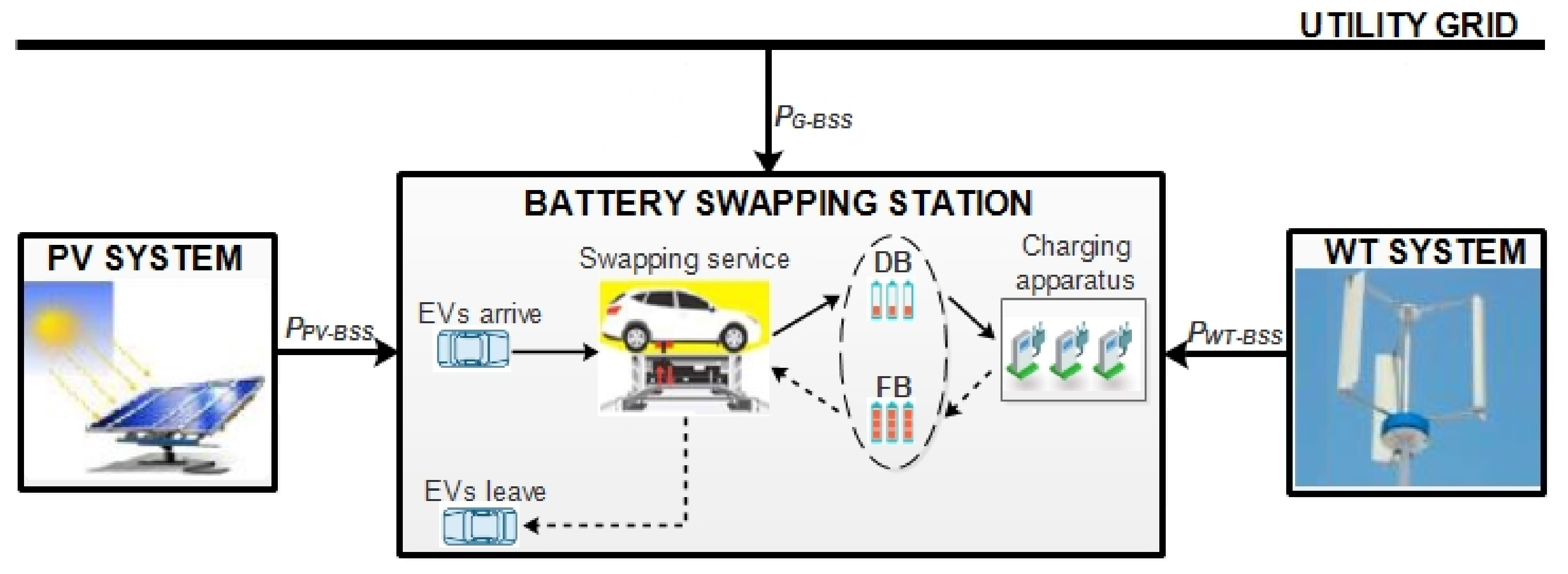
Figure 2.
Wind generator power curve.
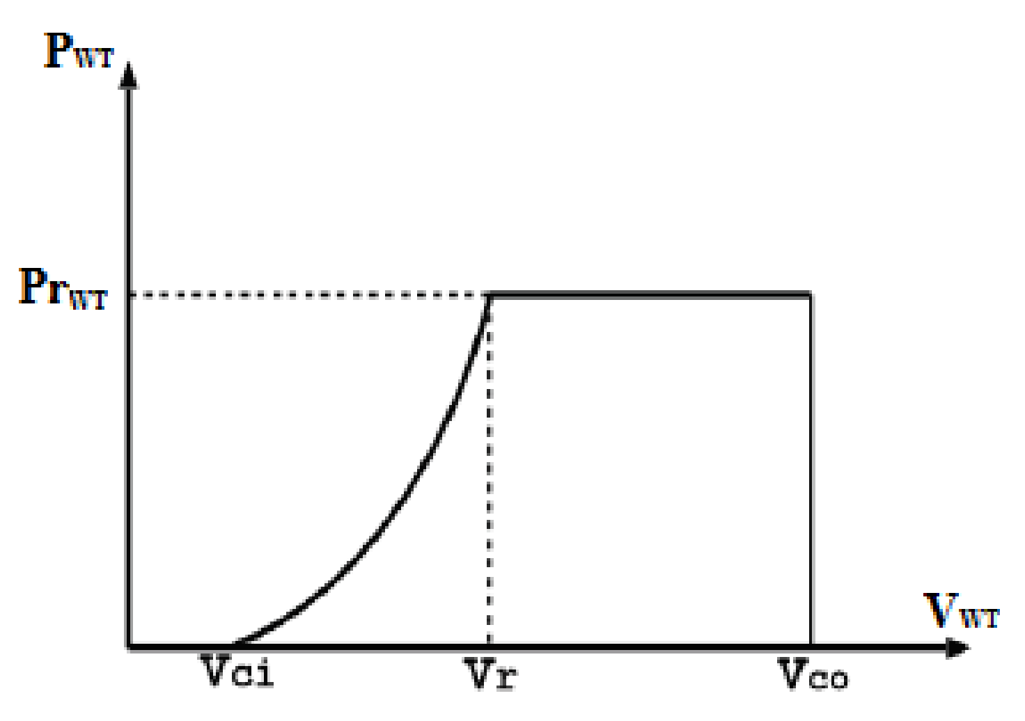
Figure 3.
Charging patterns of electric vehicles battery swapping station.
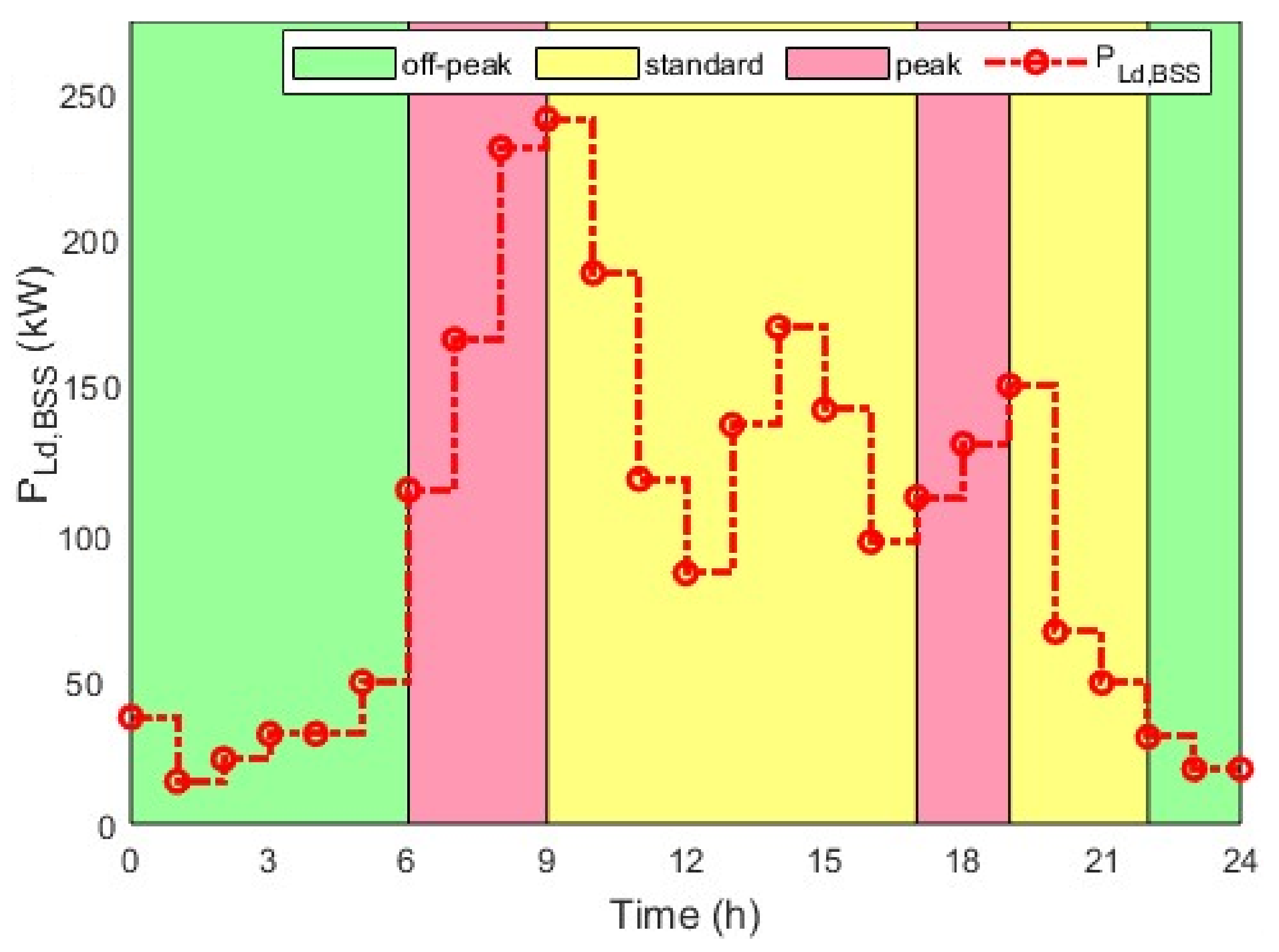
Figure 4.
Average hourly wind speed.
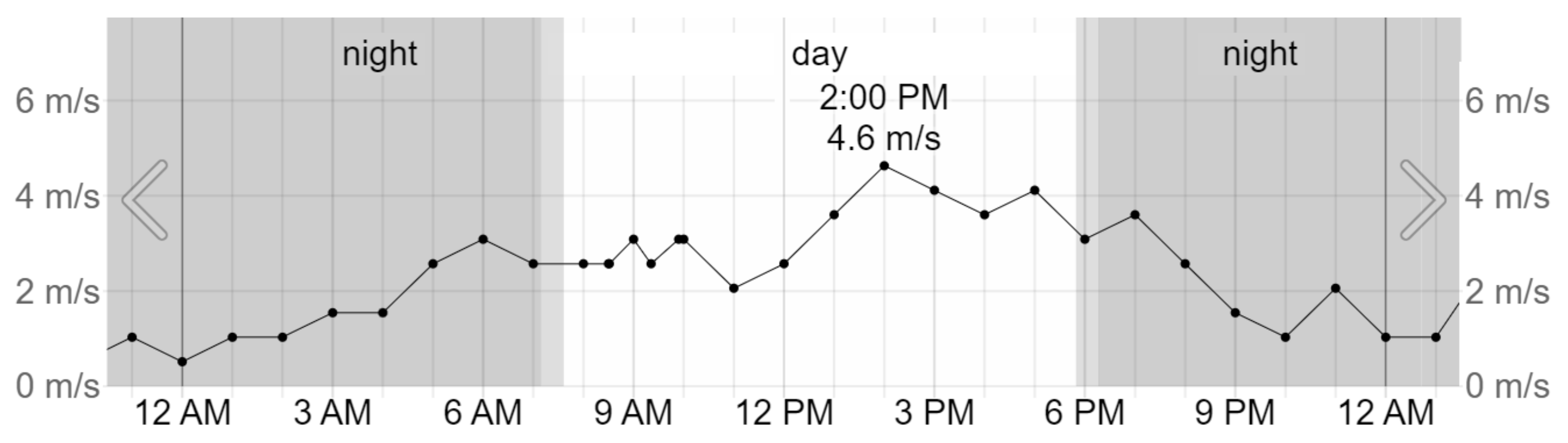
Figure 5.
Monthly average wind speed.
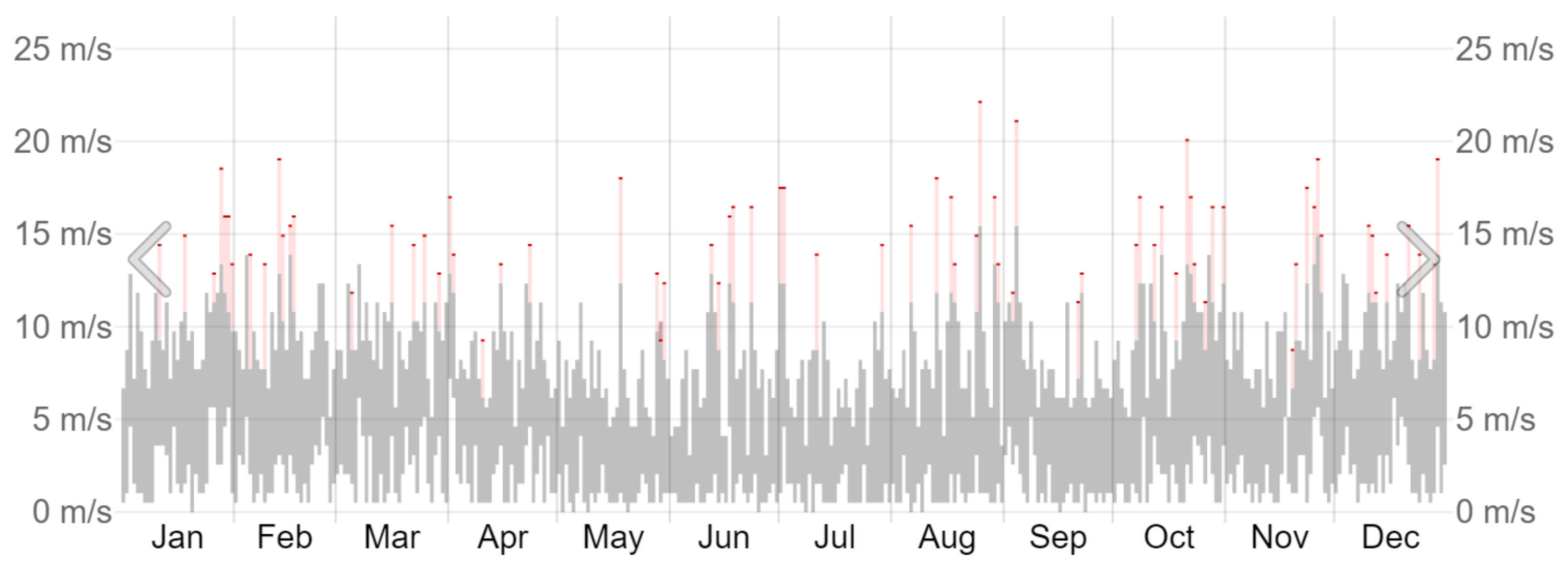
Figure 6.
Daily average shortwave solar power.
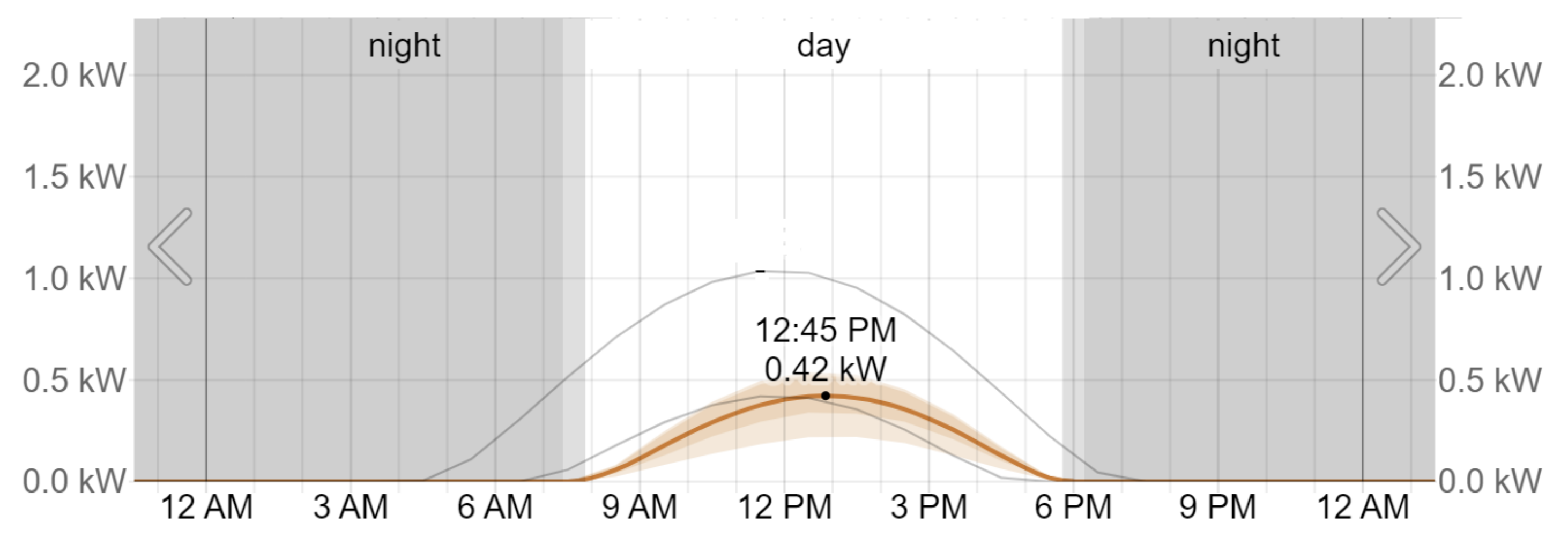
Figure 7.
Monthly average shortwave solar power.
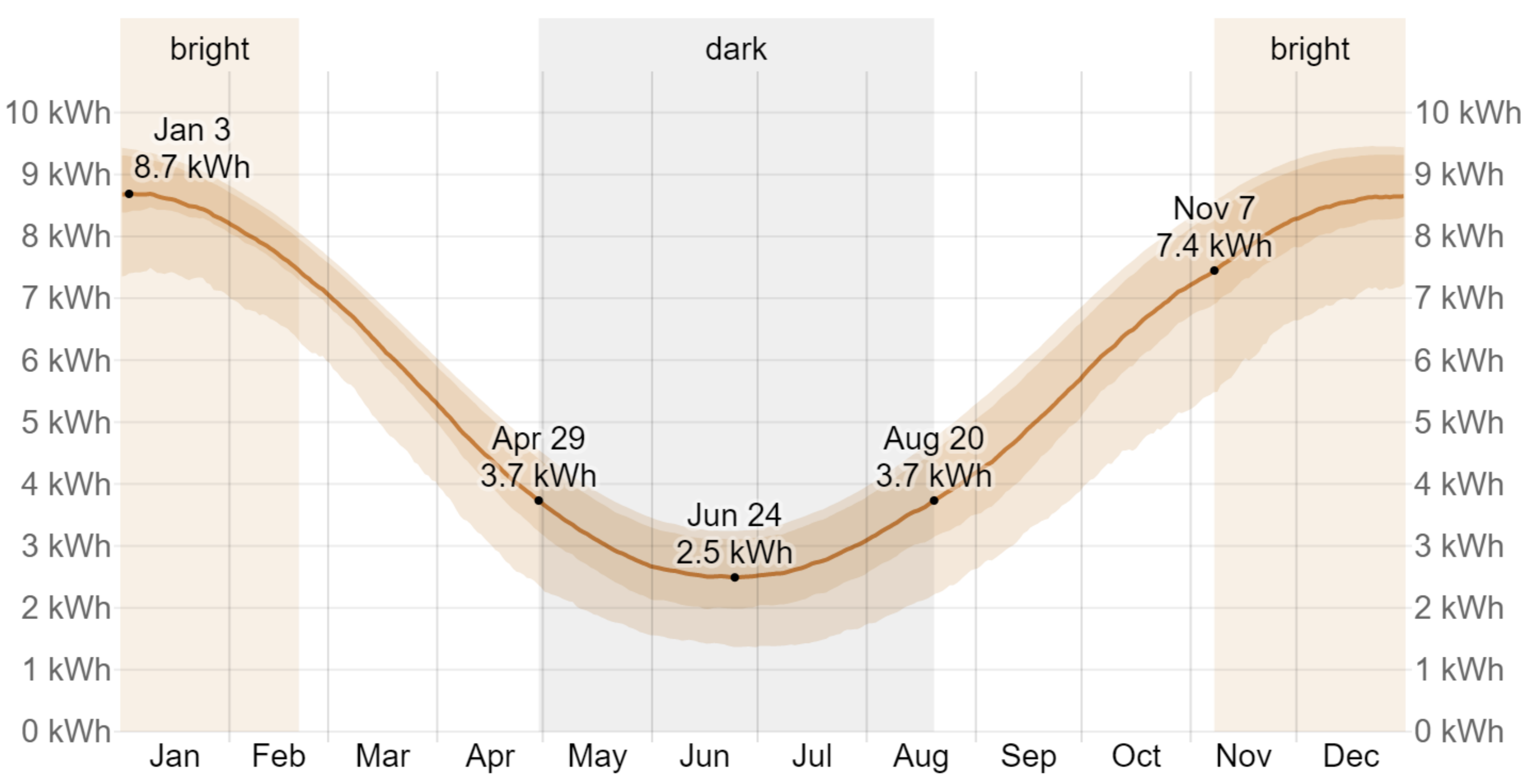
Figure 8.
Wind and photovoltaic power generated by the hybrid systems.
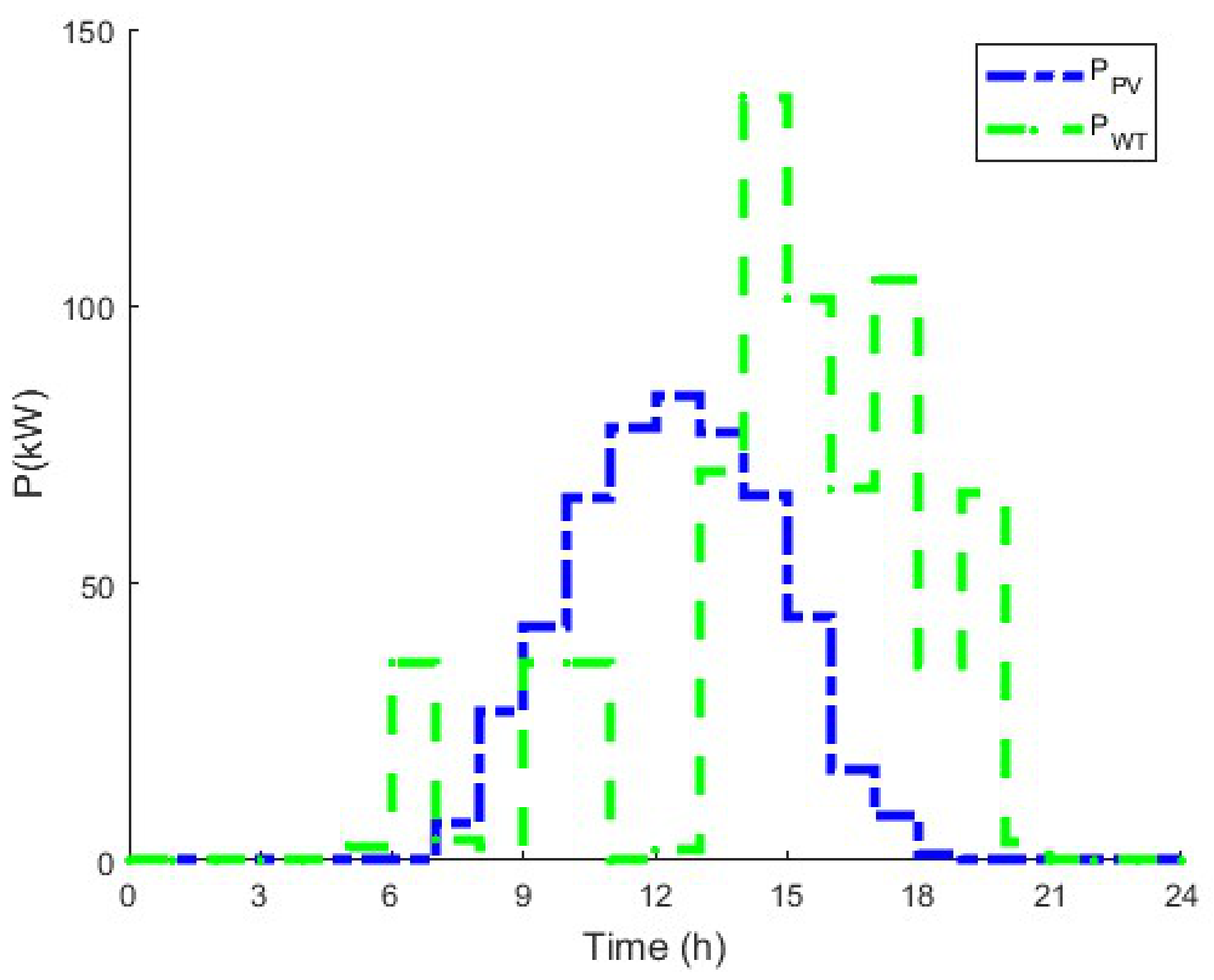
Figure 9.
Load side power flows at EV-BSS.
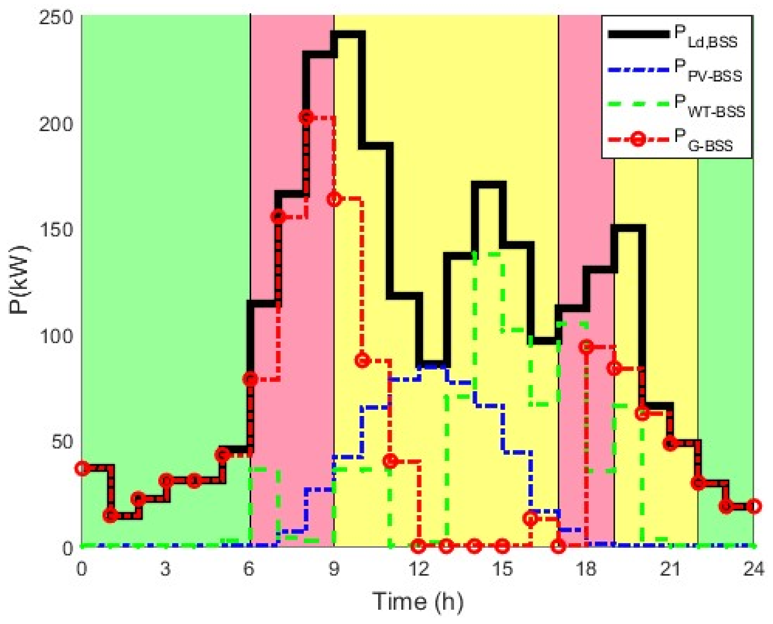

Table 1.
Simulation parameters used in this paper.
| Parameters | Symbol | Values |
|---|---|---|
| Installation lifetime | 20 years | |
| Sampling period | N | 24 |
| Sampling time | 1 h | |
| Weighting factor | 0.5 | |
| Upper bound | ||
| Lower bound | ||
| Inflation rate | r | 4.60% |
| Interest rate | i | 8.25% |
| PHOTOVOLTAIC SYSTEMS | ||
| Lifetime of the PV system | 25 years | |
| Rated power of the PV panel | 0.545 kW | |
| Conversion efficiency of the PV panel | 19.4% | |
| Rated efficiency of the PV panel | 18.1% | |
| Initial cost of the PV panel | 3 199.99 ZAR | |
| Annual O & M cost of PV | 1% of | |
| Capital cost of the solar PV per kW | 8 220.16 ZAR/kW | |
| WIND TURBINE SYSTEMS | ||
| Lifetime of the WT system | 25 years | |
| Rated power of the WT generator | 8 kW | |
| Rated WT speed | 12 m/s | |
| Cut-in WT speed | 2.5 m/s | |
| Cut-out WT speed | 25 m/s | |
| WT gearbox efficiency | 90% | |
| WT generator efficiency | 80% | |
| Air density | 1.225 kg/m3 | |
| WT power coefficient | 0.48 | |
| Initial cost of the WT | 10 580,63 ZAR | |
| Annual O & M cost of WT | 5% of | |
| Capital cost of the WT per kW | 15 403 ZAR/kW | |
| INVERTER | ||
| Lifetime of the inverter | 15 Years | |
| Efficiency of the inverter | 98% | |
| Inverter factor | 1.25 | |
| Initial cost of the inverter | 38 860.00 ZAR | |
| Capital cost of inverter per kW | 3 108.80 ZAR/kW |
Table 2.
Simulation results of the proposed system.
| Number of WTs | Number of PV panels | Total life cycle cost |
|---|---|---|
| 64 | 420 | 1 963 520.12 ZAR |
Table 3.
Daily and annual cost savings of the proposed system.
| Baseline cost | Optimal cost | Cost saving | |
|---|---|---|---|
| Daily | 7 676.39 ZAR | 4 483.53 ZAR | 3 192.5 ZAR |
| Annualized | 1 165 262.5 ZAR |
Table 4.
Costs components of the proposed system.
| Components | Costs (ZAR) |
|---|---|
| Wind turbines | 677 160.32 |
| Solar photovoltaic | 1 286 359.80 |
| Inverters | 77 720 |
| Installation cost | 649 975,98 |
| Accessories | 3 000 000 |
| Total investment capital cost | 5 691 216.10 |
Table 5.
Life cycle cost analysis and payback period of the proposed system (Total investment capital cost is ZAR 5 691 216.10.). Payback is 5 years plus 6 months (6.45636)
Table 5.
Life cycle cost analysis and payback period of the proposed system (Total investment capital cost is ZAR 5 691 216.10.). Payback is 5 years plus 6 months (6.45636)
| Years | Annual O & M cost (ZAR) | Annual optimal cost benefit (ZAR) | Total | Discount factor (1+d) | Discounted cash flows | Cumulative cash flows |
|---|---|---|---|---|---|---|
| 0 | 1.00 | (5 691 216.10) | (5 691 216.10) | |||
| 1 | (46 721.61) | 1 165 390.25 | 1 118 668.64 | 0.96 | 1 079 275.10 | (4 611 941.01) |
| 2 | (47 389.73) | 1 182 055.33 | 1 134 665.60 | 0.93 | 1 056 158.93 | (3 555 782.07) |
| 3 | (48 067.40) | 1 198 958.72 | 1 150 891.32 | 0.90 | 1 033 537.87 | (2 522 244.20) |
| 4 | (48 754.77) | 1 216 103.83 | 1 167 349.07 | 0.87 | 1 011 401.32 | (1 510 842.89) |
| 5 | (49 451.96) | 1 233 494.12 | 1 184 042.16 | 0.84 | 989 738.89 | (521 104.00) |
| 6 | (50 159.12) | 1 251 133.08 | 1 200 973.96 | 0.81 | 968 540.43 | 447 436.43 |
| 7 | (50 876.40) | 1 269 024.29 | 1 218 147.89 | 0.78 | 947 796.00 | 1 395 232.43 |
| 8 | (51 603.93) | 1 287 171.33 | 1 235 567.40 | 0.75 | 927 495.88 | 2 322 728.31 |
| 9 | (52 341.87) | 1 305 577.88 | 1 253 236.02 | 0.72 | 907 630.56 | 3 230 358.87 |
| 10 | (53 090.35) | 1 324 247.65 | 1 271 157.29 | 0.70 | 788 190.71 | 4 018 549.58 |
| 11 | (53 849.55) | 1 343 184.39 | 1 289 334.84 | 0.67 | 869 167.24 | 4 887 716.82 |
| 12 | (54 619.60) | 1 362 391.92 | 1 307 772.33 | 0.65 | 850 551.21 | 5 738 268.03 |
| 13 | (55 400.66) | 1 381 874.13 | 1 326 473.47 | 0.63 | 832 333.90 | 6 570 601.93 |
| 14 | (56 192.89) | 1 401 634.93 | 1 345 442.04 | 0.61 | 814 506.78 | 7 385 108.72 |
| 15 | (56 996.44) | 1 421 678.31 | 1 364 681.86 | 0.58 | 797 061.48 | 8 182 170.20 |
| 16 | (57 811.49) | 1 442 008.31 | 1 384 196.82 | 0.56 | 779 989.84 | 8 962 160.04 |
| 17 | (58 638.20) | 1 462 629.03 | 1 403 990.83 | 0.54 | 763 283.83 | 9 725 443.87 |
| 18 | (59 476.72) | 1 483 544.62 | 1 424 067.90 | 0.52 | 746 935.64 | 10 472 379.50 |
| 19 | (60 327.24) | 1 504 759.31 | 1 444 432.07 | 0.51 | 730 937.60 | 11 203 317.10 |
| 20 | (61 189.92) | 1 526 277.37 | 1 465 087.45 | 0.49 | 715 282.20 | 11 918 599.30 |
Disclaimer/Publisher’s Note: The statements, opinions and data contained in all publications are solely those of the individual author(s) and contributor(s) and not of MDPI and/or the editor(s). MDPI and/or the editor(s) disclaim responsibility for any injury to people or property resulting from any ideas, methods, instructions or products referred to in the content. |
© 2025 by the authors. Licensee MDPI, Basel, Switzerland. This article is an open access article distributed under the terms and conditions of the Creative Commons Attribution (CC BY) license (http://creativecommons.org/licenses/by/4.0/).
Copyright: This open access article is published under a Creative Commons CC BY 4.0 license, which permit the free download, distribution, and reuse, provided that the author and preprint are cited in any reuse.


