
Submitted:
14 January 2025
Posted:
15 January 2025
You are already at the latest version
Abstract
Transformer encoders are widely used in deep learning-based time series anomaly detection due to their ability to capture temporal dependencies. Recently, many studies have attempted to improve a vanilla Transformer encoder by incorporating their novel techniques into the vanilla Transformer encoder. These advanced models have shown remarkable performance in various time series anomaly detection benchmarks. However, unlike these approaches, we argue that vanilla Transformer encoders remain undervalued. To support this claim, Through extensive experiments, we evaluated the proposed framework against advanced models on widely recognized time series anomaly detection benchmarks. The results demonstrate that our simple framework delivers performance comparable to that of the advanced models. The code for the proposed framework, along with its pre-trained weights for the benchmark datasets, is publicly available at https://github.com/chatterboy/revisitVanillaTransEncUnsupTSAD.
Keywords:
time series anomaly detection
; unsupervised learning
; vanilla transformer encoders
; careful design choices
1. Introduction
Time series anomaly detection is to identify unusual patterns or events in time series data [1,2]. This is an important problem across many domains like finance, manufacturing, and healthcare [3,4]. Due to its importance, this problem has been a focus of research for several decades. Initially, statistical methods [5,6,7,8] and machine learning methods [9,10,11,12] were studied. Recently, with advancements in deep learning, there has been increasing interest in applying deep learning models to time series anomaly detection [13]. In particular, unsupervised time series anomaly detection has attracted significant attention due to the issue of collecting abnormal data in real-world scenarios [14,17,18,19].
In unsupervised time series anomaly detection, numerous models have been proposed. Some studies have focused on capturing temporal dependencies using RNNs and LSTMs [15,20,21], while others have used CNNs and TCNs to extract temporal features locally and hierarchically [22,23,24]. Additionally, Graph Neural Networks have been employed to model complex relationships in multivariate time series data [25,26,27]. Generative models, such as Variational Autoencoders, Generative Adversarial Networks, Normalizing Flows, and Diffusion models, have also been explored. These models detect anomalies by analyzing reconstruction errors or deviations from learned data distributions [16,28]. Autoencoders, in particular, are widely adopted due to their simplicity and effectiveness in capturing temporal features [30].
Transformers, originally introduced in natural language processing (NLP), demonstrated superior performance compared to previous models [31]. Since then, it has been successfully applied across diverse domains, proving its effectiveness. Recently, the success of Transformers has driven extensive research into their application for unsupervised time series anomaly detection [32,33,34,35]. In particular, the Transformer encoder has gained attention for its ability to simultaneously capture temporal dependencies and complex patterns within time series data. However, due to the inherent complexity of time series data, many studies have attempted to improve a vanilla Transformer encoder by introducing novel techniques. These improvements have achieved superior performance on various benchmarks [32,36,37,38].
In contrast to these trends, this study revisits the potential of the vanilla Transformer encoder for unsupervised time series anomaly detection. We argue that, despite its simplicity, the vanilla Transformer encoder, when combined with thoughtful preprocessing techniques and design choices, can achieve competitive performance with state-of-the-art models. This research proposes a minimalist framework that leverages a vanilla Transformer encoder and a simple linear decoder to perform anomaly detection effectively. Our experiments demonstrate that this approach highlights the often-overlooked potential of the vanilla Transformer encoder in handling diverse time series anomlay detection tasks.
2. Materials and Methods
This work aims to revisit the potential of a vanilla Transformer encoder in unsupervised time series anomaly detection. To evaluate the capabilities of a vanilla Transformer encoder, we propose an autoencoder-based framework equipped with a vanilla Transformer encoder and a linear layer decoder(see Figure 1). This framework makes use of a simple architecture while enabling a vanilla Transformer encoder to effectively capture temporal dependencies. This framework takes time series segments, generated from (preprocessed) time series data, as input and reconstructs the taken time series segments. The proposed framework consists of the following modules: preprocessing time series, generating time series segments, segment-level normalization-denormalization, time series segment embedding, and an asymmetric encoder-decoder.
2.1. Preprocessing Time Series Data
Preprocessing plays a vital role in the development of a deep learning framework. We are concerned with normalization techniques for preprocessing in the context of unsupervised learning-based time series anomaly detection. They are used to convert the scale of time series data into a specified interval, which usually significantly impacts the performance of the anomaly detection process.
Representative normalization techniques include min-max normalization and z-score normalization. Let represent time series data, where denotes the value at the i-th time step of the j-th variable. Its normalized time series data can be expressed in , where is a normalization method which is defined as follows:
where and represent the mean and standard deviation of the j-th variable, respectively.
This study emphasizes selecting the most suitable normalization method for each dataset rather than applying a uniform approach, to better capture temporal features. In model development, we consider the following three options: no use of normalization, min-max normalization, and z-score normalization. We choose the best option by examining the performance of each option for the given dataset.
Some datasets are composed of multiple sub-datasets (see Table 1 and Table 2). For instance, the multivariate dataset MSL consists of 27 sub-datasets, and the univariate dataset ABP consists of 42 sub-datasets. For datasets consisting of multiple sub-datasets, we apply two levels of normalization sequentially: first at the sub-dataset level, followed by the dataset level, with three normalization options available at each level. Sub-dataset level normalization is performed on each sub-dataset individually, while dataset-level normalization is applied across all sub-datasets as a whole. The total nine combinations of normalization methods for the sub-dataset level and the dataset level are examined to select the best one. At inference time, parameters such as min, max, mean, and standard deviation, computed during training, are utilized.
2.2. Generating Time Series Segments
Time series datasets often consist of long sequences dynamically collected in real-world environments. These characteristics can make it difficult to directly feed raw time series data into an outlier detection model. To address this, techniques for generating fixed-length segments from the original data are employed, facilitating easier analysis and processing by the model.
The windowing technique is a commonly used method for generating time series segments in unsupervised anomaly detection for time series data. It involves copying fixed-length segments from an original time series data at regular intervals using a sliding window. Varying the window length and stride enables the generation of different sets of time series segments from the data. The process of generating a full set of time series segments from preprocessed data using the windowing technique can be outlined as follows:
where is a window function, , and denote the time series sigement and its preprocessed dataset, respectively.
The optimal window length and stride size for capturing temporal dependencies effectively can vary across datasets. To address this, we adopt window lengths and stride sizes tailored to each dataset. Furthermore, stride size can be applied differently during training and evaluation. During evaluation, the stride size matches the window length, following the non-overlapping approach used in prior studies such as [20,37,38,39]. In contrast, during training, the stride size is selected based on whether an overlapping or non-overlapping approach is more effective for capturing temporal dependencies. This approach ensures efficient temporal pattern extraction during training.
2.3. Segment-Level Normalization and Denormalization
Real-world time series data are often non-stationary, with statistical properties that change over time. This non-stationarity poses significant challenges in extracting meaningful temporal features. Since time series segments are derived from non-stationary data, they inherently retain this non-stationarity. To address these challenges, we use a segment-level normalization and denormalization technique, designed to effectively capture temporal dependencies in non-stationary time series segments. As shown in Figure 1, the normalization is applied to time series segments prior to their embedding. The embedded time series segments pass through the encoder and the corresponding time series segments are reconstructed by the decoder. The reconstructed one is denormalized into the scale of original time series segments.
We employ a reversible instance normalization method [40], originally proposed for time series forecasting to address distribution shifts between training and testing datasets, for normalizing and denormalizing time series segments. Given batched time series segments with batch size B, the sequence length L and the number of variables V, the normalization method is applied to multivariate time series segments as follows:
where represents the normalized time series segments, and denote the mean and standard deviation of the data points of the j-th variable within a time series segment i, and and are learnable parameters used for scaling and shifting of the j-th variable. This normalization might mitigate the impact of non-stationality, while preserving the temporal characteristics of time series segments.
The encoder and decoder are trained to reconstruct the normalized time series segments at the output of the decoder. For normalized time series segments reconstructed by the decoder, denormalization is carried out as follows:
where represents the final denormalized reconstructed time series segments produced by the model, while represents the normalized reconstructed time series segments generated by the decoder.
2.4. Time Series Segment Embedding
Time series segment embedding is needed to transform time series segments into a format suitable for the proposed autoencoder-based architecture which consists of the encoder and decoder shown in Figure 1. The embedding module converts the data points of dimension V within time series segments into real-valued vectors of dimension F. To capture both individual data point information and short-term temporal dependencies within time series segments, we use a 1D convolutional layer for embedding. That is, the embedding method generates an embedding vector e by considering individual data points along with their neighboring data points for a time series segment .
where is a batch of B sequences, where each sequence consists of L embedding vectors with a feature dimension of F. The 1D convolutional layer consists of F kernels, each with a length of 3, a stride of 1, and no bias term, to generate an embedding vector of dimension F. Zero padding is applied to ensure that the sequence length of the embedded time series segment matches that of the original time series segment.
Additionally, we choose not to use positional encoding (PE), which is commonly employed in Transformers to incorporate positional information for extracting position-based features. This decision is based on two key considerations. First, positional encoding works by injecting additional positional information into the data. However, this process may lead the model to interpret the sequential flow of the data based on the positional encoding rather than its original order. As a result, the model may fail to properly learn the natural sequential relationships in the data. In reconstruction-based methods, preserving the original sequence is crucial, and such distortions can negatively impact reconstruction performance. Second, a reconstruction model, such as an autoencoder, aims to reproduce the input data as accurately as possible. Adding positional encoding introduces new patterns to the data, which might cause the model to learn these patterns inappropriately or to overlook essential structural information from the original data by overemphasizing positional differences. This may impair the model’s reconstruction performance, resulting in degrading its anomaly detection capabilities. To assess the impact of positional encoding, we have conducted an ablation study as part of our analysis (see Subsection 3.4).
2.5. Asymmetric Autoencoder
Autoencoders are widely used in unsupervised time series anomaly detection because of their simplicity and capability to reconstruct input data. An autoencoder consists of two components: an encoder and a decoder. The encoder extracts features from the input data, while the decoder reconstructs the input data from these extracted features. According to Wang et al. [41], an overly powerful decoder can hinder the encoder’s ability to effectively capture meaningful features. This is because the decoder may accurately reconstruct the input data during training, even when relying on uninformative features such as random noise.
To mitigate this issue, we propose an asymmetric autoencoder design where the encoder is more complex and parameter-rich, while the decoder is kept simpler with fewer parameters. This asymmetry ensures that the decoder focuses solely on reconstruction, allowing the encoder to effectively capture rich and informative temporal features from the time series segments. Specifically, we use a vanilla Transformer encoder for the encoder and a linear layer for the decoder.
Given a batch of embedding vector sequences , a vanilla Transformer encoder produces a batch of hidden vector sequences as follows:
where is the output of the last encoder block in a vanilla Transformer encoder. Then, a decoder reconstructs normalized time series segments for given hidden vector sequences.
The decoder, implemented as a linear layer, transforms each hidden vector from the encoder into a data point within a normalized time series segment, as follows:
where is a weight matrix for the decoder. The decoder processes each hidden vector generated by the encoder to reconstruct the normalized time series segment corresponding to the input time series segment provided to the encoder.
2.6. Training
The proposed framework is an autoencoder-based model designed to reconstruct given time series segments. To achieve this, we employ a reconstruction-based training approach that minimizes the discrepancy between the input and the reconstructed output. Specifically, the model is trained to reduce the difference between the input time series segments and the corresponding reconstructed segments generated by the framework. Let represent the input time series segments, and let denote the reconstructed segments. The model is optimized using the following loss function:
where B is batch size, and and denote the b-th segments of and , respectively.
2.7. Evaluation
We use an evaluation protocol commonly used in reconstruction-based methods. The protocol consists of three steps: first, computing anomaly scores; second, predicting whether each timestamp is normal or abnormal; and third, evaluating the predictions using standard evaluation metrics.
Various methods exist for computing anomaly scores in reconstruction-based approaches. We utilize the anomaly scoring method proposed in the literature [36,37,38,39]. For a given data point from a batched time series segment and its reconstructed counterpart produced by the trained model, the anomaly score at timestamp t is computed as follows:
To predict the anomaly status at each timestamp t within the time series data , we compute it as follows:
Here, represents the anomaly status prediction, where , and is the threshold used to determine whether a data point is anomalous or normal. The threshold is a critical parameter for accurate predictions. Among the various methods available for threshold selection, we adopt the approach used in the previous comparative studies [37,38,39].
To evaluate the model’s performance, we utilize a range of metrics. We employ Precision, Recall, and F1 score for experiments on multivariate datasets, which are widely used in unsupervised time series anomaly detection. Additionally, we use Point Adjustment (PA) [42], a post-processing method that considers an entire anomalous segment correctly identified if at least one data point within the segment is detected as anomalous. PA-based metrics are applied to both the proposed framework and the comparative models [36,37,38,39] for fair evaluation.
However, PA-based metrics have limitations in fully capturing model performance [43,44]. To address these issues, we adopt the affiliation metrics [45] in experiments with univariate datasets. These metrics, designed to overcome the shortcomings of PA-based metrics, include affiliation Precision, affiliation Recall, and affiliation F1 score, providing a more robust evaluation.
3. Comparative Experiments and Results
3.1. Benchmark Datasets
This section outlines the datasets utilized to evaluate the proposed framework. The evaluation includes both multivariate and univariate time series datasets widely used.
3.1.1. Multivariate datasets
We use six multivariate time series anomaly detection benchmarks, as described in Table 1. The MSL [15] contains telemetry data with labeled anomalies from the Mars Science Laboratory rover. The SMAP [15] includes telemetry and anomaly labels from the Soil Moisture Active Passive satellite. The SMD [16] is a labeled multivariate time series dataset containing metrics like CPU and memory usage from 28 server machines over 5 weeks. The PSM [46] features anonymized server metrics from eBay spanning 13 weeks of training and 8 weeks of testing. The GECCO [2] focuses on drinking water quality monitoring, providing multivariate time series data with physical and chemical properties. The SWAN-SF [2] includes multivariate time series data on extreme space weather conditions for space weather analysis.

Table 1.
Description of multivariate time series anomaly detection benchmark datasets.
| # sub-datasets | # dimensions | # training data points | # test data points | Anomaly ratio (%) | |
| MSL | 27 | 55 | 58,317 | 73,729 | 10.53 |
| SMAP | 54 | 25 | 138,004 | 435,826 | 12.84 |
| SMD | 28 | 38 | 708,405 | 708,420 | 4.16 |
| PSM | 1 | 25 | 132,481 | 87,841 | 27.76 |
| GECCO | 1 | 9 | 69,260 | 69,261 | 1.05 |
| SWAN-SF | 1 | 38 | 60,000 | 60,000 | 32.60 |
3.1.2. Univariate datasets
We employ nine univariate time series anomaly detection benchmark datasets, described in Table 2. These datasets are derived from the UCR Anomaly Archive [47], following the categorization by Goswami et al. [48]. The UCR Anomaly Archive consists of 250 sub-datasets, each originating from a specific domain. Goswami et al. [48] grouped these sub-datasets into nine distinct domains: ABP, Acceleration, Air Temperature, ECG, EPG, Gait, NASA, Power Demand, and RESP. To construct the datasets, we concatenated all sub-datasets within each domain.
Table 2.
Description of univariate time series anomaly detection benchmark datasets.
| # sub-datasets | # training data points | # test data points | Anomaly ratio (%) | |
| ABP | 42 | 1,036,746 | 1,841,461 | 0.37 |
| Acceleration | 7 | 38,400 | 62,337 | 1.71 |
| Air Temperature | 13 | 52,000 | 54,392 | 0.82 |
| ECG | 91 | 1,795,083 | 6,047,314 | 0.38 |
| EPG | 25 | 119,000 | 410,415 | 0.45 |
| Gait | 33 | 1,157,571 | 2,784,520 | 0.38 |
| NASA | 11 | 38,500 | 86,296 | 0.86 |
| Power Demand | 11 | 197,149 | 311,629 | 0.61 |
| RESP | 17 | 868,000 | 2,452,953 | 0.12 |
3.2. Baselines
To assess the effectiveness of the proposed framework, we compare it with recent advanced deep learning methods for unsupervised time series anomaly detection. For multivariate datasets, the baseline methods include Anomaly Transformer [37], DCdetector [39], MEMTO [38], and AnomalyLLM [36]. For univariate datasets, the comparisons feature TS-TCC [49], THOC [20], NCAD [50], and AnomalyLLM [36].
3.3. Implementation Details
The proposed framework was implemented using Python 3.8.19 and PyTorch 2.1.0. Training and evaluation were conducted on a single NVIDIA A100 GPU, utilizing the Adam optimizer [51]. The hyperparameter configurations for the multivariate and univariate datasets are detailed in Table A1 and Table A2, respectively. Key hyperparameters were determined through a grid search, while other parameters were set to commonly used default values.
3.4. Main Results
Table 3 presents the F1 scores comparing the proposed vanilla Transformer encoder-based model with state-of-the-art time series anomaly detection methods, including Anomaly Transformer, DCdetector, MEMTO, and AnomalyLLM, across the six multivariate time series datasets.
The results for the proposed model were obtained following the aforementioned experimental procedures, while the results for the other models were taken from their respective publications. The findings reveal that the proposed model achieved competitive performance across most datasets, with superior results on some. Specifically, it recorded the highest F1 scores of 0.975 and 0.920 on SMAP and GECCO, respectively. For SMD, PSM, and SWAN-SF, it achieved the second-highest performance, following AnomalyLLM. In particular, on GECCO, the proposed model outperformed both DCdetector and AnomalyLLM by a substantial margin.
These results highlight that, despite its relatively simple architecture, the proposed model delivers performance comparable to or better than more advanced models. Through thoughtful design choices, the vanilla Transformer encoder-based model effectively captures the temporal dependencies inherent in time series data. Further details on the experimental results are provided in Table A3.
Table 4 presents the Affiliation F1 scores comparing the proposed vanilla Transformer encoder-based model with state-of-the-art time series anomaly detection methods, including THOC, NCAD, and AnomalyLLM, across the nine univariate time series datasets. The results of the proposed model were obtained using the outlined experimental procedures, while those for the other models were sourced from the experiments in AnomalyLLM [36].
The findings show that, with few exceptions, the proposed model demonstrated competitive or superior performance in most datasets. Notably, it achieved the highest scores of 0.966, 0.802, and 0.763 on Acceleration, ECG, and RESP, respectively. For datasets such as ABP, Air Temperature, Gait, NASA, Power Demand, and Average, the model delivered the second-best performance. Although the proposed model showed a noticeable performance gap compared to AnomalyLLM on ABP and EPG, it performed competitively or even better on the remaining datasets.
As with the multivariate dataset experiments, these results confirm that the proposed model, despite its relatively simple architecture, achieves performance comparable to or exceeding that of advanced methods. This shows that with thoughtful design choices, a vanilla Transformer encoder-based model can effectively capture temporal features. Additional details on the experimental results are provided in Table A4.
3.5. Ablation Study
We conducted an ablation study to evaluate the impact of the key design principles underlying the proposed framework. These principles include: (1) segment-level normalization and denormalization, (2) the use of positional encoding, and (3) preprocessing of time series data.
3.5.1. Segment-level normalization and denormalization
To evaluate the effectiveness of segment-level normalization and denormalization, we assessed the model’s performance with and without RevIN. For this analysis, three multivariate datasets (MSL, SMAP, and SMD) and three univariate datasets (ECG, Gait, and RESP) were selected. The F1 score was used as the evaluation metric for the multivariate datasets, while the affiliation F1 score was applied for the univariate datasets.
Table 5 shows the F1 scores for the multivariate datasets, and Table 6 presents the affiliation F1 scores for the univariate datasets. In the experiments with the multivariate datasets, incorporating RevIN consistently led to improved performance across all datasets. Similarly, in the univariate dataset experiments, RevIN generally achieved superior performance. These findings demonstrate that employing RevIN can enhance the performance of both multivariate and univariate anomaly detection tasks.
RevIN has been develped to address distribution shift issues that occur between training and testing datasets in time series forecasting. In this study, we used RevIN not only to mitigate distribution shifts between training and testing datasets but also to alleviate distribution shifts between time series segments in window-based anomaly detection. Such segment-level distribution shifts can prevent a model from effectively learning general temporal patterns during training. By addressing this issue, RevIN facilitates the efficient capture of general temporal patterns.
3.5.2. Positional Encoding
The analysis revealed that incorporating positional encoding (PE) does not consistently improve the model’s performance in time series anomaly detection. Experiments on multivariate datasets, such as MSL, SMAP, and SMD, produced mixed results when absolute positional encoding (APE) or learnable PE was applied. Notably, the vanilla Transformer encoder achieved the highest F1 scores without any form of PE, as shown in Table 5. This indicates that preserving the temporal context in its original form may be more effective for reconstruction-based anomaly detection tasks.
Reconstruction tasks often rely on maintaining the integrity of the temporal context. Adding positional information can cause the model to differentiate features unnecessarily, potentially leading to overfitting on anomalous data. For univariate datasets, such as ECG, Gait, and RESP (see Table 6), the exclusion of PE also resulted in higher affiliation F1 scores. This aligns with the hypothesis that PE may introduce additional complexity, counterproductive for models focused on reconstructing temporal patterns.
Overall, these findings underscore that positional encoding is not essential for the vanilla Transformer encoder in this task. Instead, direct modeling of temporal dependencies can yiedld better results.
3.5.3. Preprocessing Time Series Data
Preprocessing strategies played a crucial role in determining the model’s performance. The experiments examined various preprocessing combinations of normalization at both the dataset and sub-dataset levels, including min-max normalization and z-score normalization. The results in Table 7 and Table 8 provide the following key insights: For all the multivariate datasets, highest F1 scores are achieved without using any normalization methods at sub-dataset-level and dataset-level normalizations. For the univariate datasets, different normalization methods at sub-dataset-level and dataset-level normalizations produced the best affiliation F1 scores.
Choosing the preprocessing techniques like normalization that align with the specific characteristics of a dataset is crucial for preserving the integrity of its temporal structure. Proper preprocessing strategies, for multivariate and univariate datasets, enhance the model’s ability to distinguish normal patterns from anomalies, thereby improving reconstruction accuracy. These findings advocate for a tailored approach to preprocessing in time series anomaly detection, emphasizing its significant impact on model performance.
3.6. Hyperparameter Sensitivity
We performed a hyperparameter sensitivity analysis for the key parameters of our proposed framework. Figure 2 presents the results of this analysis.
For the training window stride, the results indicate that the framework demonstrates robust performance within a specific range. However, performance declines significantly as the stride decreases, especially in the MSL and SMD datasets. This drop may result from variations in the time series segments generated according to the training window stride.
Regarding the window length, the framework exhibits high sensitivity to this parameter. For the MSL and SMAP datasets, performance tends to decrease as the window length increases. Conversely, in the SMD dataset, shorter window lengths lead to poorer performance. Additionally, in the SMAP dataset, performance declines when the window length deviates from 50, either shorter or longer. Since window length directly affects the generation of training and testing time series segments, it is a critical hyperparameter. Given that the optimal window length varies across datasets, selecting an appropriate value is crucial for achieving the best results.
For the number of heads in the Transformer-based encoder, this parameter appears to have minimal impact on model performance. While employing multiple attention heads allows the model to capture diverse dependencies, the results suggest that increasing the number of heads does not enhance performance. This indicates that effective anomaly detection can be achieved with a smaller number of dependencies.
The model dimension size shows varying effects depending on the dataset. For MSL and SMAP, performance decreases as the model dimension size increases. In contrast, for SMD, performance deteriorates when the model dimension size is either smaller or larger than 128. In PSM, performance remains unchanged across all model dimension sizes. These results highlight the need to carefully tune the model dimension size for optimal performance.
The impact of the number of encoder blocks varies depending on the dataset. For SMAP and PSM, performance remains almost unchanged regardless of the number of encoder blocks. In contrast, SMD and PSM exhibit greater performance fluctuations, indicating that this parameter can affect model performance in specific datasets.
The learning rate results show trends similar to the number of encoder blocks. In SMAP and PSM, performance is largely unaffected by changes in the learning rate. However, in SMD and PSM, significant variations in performance are observed, indicating that the learning rate is also an important hyperparameter.
Lastly, the dropout ratio results suggest that the framework achieves robust performance across different dropout ratios. Even in MSL, where the largest performance variation is noted, the changes are relatively minor.
4. Discussion
This work highlights the potential of a vanilla Transformer encoder with carefully selected design choices for unsupervised time series anomaly detection. Despite its simplicity, the proposed framework delivers performance that is competitive with, and in some cases exceeds, state-of-the-art models across various benchmark datasets. Notably, our framework achieved overall performance comparable to the SOTA model, AnomalyLLM, which relies on abnormal data injection [50,52,53] — a technique that synthesizes abnormal data from normal data during training. In contrast, our framework uses only normal data for training. These findings underscore the viability of a vanilla Transformer encoder as an effective model for unsupervised time series anomaly detection.
Transformers require effective training strategies due to their limited inductive bias [54]. To address this, prior studies have introduced various architectural modifications. For instance, Anomaly Transformer added an extra branch to the Transformer encoder to distinguish dependencies between normal and abnormal data [37]. DCdetector developed a two-tower model with multi-head attention to simultaneously capture two types of dependencies: point-level and patch-level [39]. MEMTO incorporated a memory module to encode prototypical features [38], while AnomalyLLM implemented several architectural adjustments to efficiently model temporal patterns [36].
In contrast to these approaches, we propose a straightforward yet effective framework built on a vanilla Transformer encoder without any architectural changes. Instead, our approach emphasizes optimizing design choices such as preprocessing, time series segmentation, omitting positional encoding, segement-level normalization and demormalization, and fine-tuning hyperparameters. Comprehensive evaluations on multiple benchmark datasets for unsupervised time series anomaly detection demonstrate the effectiveness of our proposed framework.
While our proposed framework demonstrated promising results, some limitations remain. First, unsupervised time series anomaly detection is inherently challenging due to the absence of abnormal data in the training dataset [33]. With only normal data available for training, it becomes difficult to optimize hyperparameters, like the threshold in Eq.(11), that are sensitive to abnormal data.
Second, our evaluation of multivariate datasets in the experiments was conducted using the point adjustment (PA) method [42], which is known to potentially overestimate model performance [43,44]. To ensure fair comparisons with other models, we applied the same PA method as used in prior studies. However, for univariate datasets, we employed affiliation metrics [45], which are independent of the PA method, to provide a more reliable assessment of our framework’s performance in comparison to other models.
Third, we evaluated our proposed framework using a non-overlapping window evaluation protocol, where the window step size matches the window length. All the compared methods followed the same protocol for performance evaluation. In addition to the non-overlapping window protocol [20,36,37,38,39], some studies use overlapping window evaluation protocols. For example, a step size of 1 is employed in certain methods [26,27,33,55,56,57]. These differences in window step sizes during evaluation make direct comparisons across studies more challenging.
Lastly, we found that adjusting the window step size during training proved effective. However, keeping the step size fixed during the generation of time series segments restricts the model’s ability to capture the diverse temporal features present in time series data. This limitation may have adversely contributed to the significant performance gap observed compared to AnomalyLLM on certain univariate datasets.
Future research should address the limitations identified in this study. First, the reliance on training datasets containing only normal data restricts the model’s ability to generalize to diverse anomaly patterns. Incorporating semi-supervised or self-supervised learning techniques could improve the model’s capacity to handle unseen anomalies. Additionally, the evaluation methodology, which relies on the point adjustment method and non-overlapping window protocols, could be enhanced by exploring alternative metrics and approaches to ensure more comprehensive and equitable model comparisons. Investigating dynamic or adaptive windowing strategies may further enhance the detection of temporal patterns. Lastly, extending the framework to accommodate more diverse datasets and application scenarios, including resource-constrained environments, could improve its practicality and scalability.
5. Conclusions
This study revisited the potential of a vanilla Transformer encoder for unsupervised time series anomaly detection. By designing a straightforward yet effective autoencoder-based framework, we demonstrated that a vanilla Transformer encoder, when paired with thoughtful design choices, can deliver performance that is competitive with or even surpasses advanced state-of-the-art models across various univariate and multivariate benchmark datasets. Our findings highlight that the key design components, such as segment-level normalization and denormalization, omission of positional encoding, and careful hyperparameter configuration, play crucial roles in the model’s success. Despite its simplicity, the proposed framework effectively captures temporal dependencies for time series anomaly detection, highlighting the often-underestimated value of vanilla Transformer encoders.
Author Contributions
Conceptualization, C.S.Han and K.M.Lee; methodology, C.S.Han and K.M.Lee; software, C.S.Han; validation, C.S.Han, H.W.Kim. and K.M.Lee; formal analysis, C.S.Han and K.M.Lee; investigation, K.M.Lee; resources, H.W.Kim. and K.M.Lee; data curation, C.S.Han; writing—original draft preparation, C.S.Han; writing—review and editing, K.M.Lee; visualization, C.S.Han; supervision, C.S.Han; project administration, K.M.Lee; funding acquisition, H.W.Kim and K.M.Lee. All authors have read and agreed to the published version of the manuscript.
Funding
This work was supported by Innovative Human Resource Development for Local Intellectualization program through the Institute of Information & Communications Technology Planning & Evaluation (IITP) grant funded by the Korea government (MSIT) (IITP-2024-2020-0-01462, 20%), the National Research Foundation of Korea (NRF) grant funded by the Korea government (MSIT) (No. 2022R1A5A8026986, 80%).
Institutional Review Board Statement
Not applicable.
Informed Consent Statement
Not applicable.
Data Availability Statement
We have used the benchmarks which are publicly available.
Conflicts of Interest
The authors declare no conflicts of interest.
Abbreviations
The following abbreviations are used in this manuscript:
| 1D | one-dimensional |
| ABP | Arterial blood pressure benchmark |
| APE | Absolute Positional Encoding |
| CNN | Convolutional Neural Network |
| ECG | Electrocardiogram benchmark |
| EPG | Electrical Penetration Graph benchmark |
| GECCO | Genetic and Evolutionary Computation Conference benchmark |
| GRU | Gated Recurrent Unit |
| LSTM | Long Short Term Memory |
| MSL | Mars Science Laboratory benchmark |
| PA | Point Adjustment |
| PE | Positional Encoding |
| PSM | Pooled Server Metrics benchmark |
| RESP | Respiration benchmark |
| RevIN | Reversible Instance Normalization |
| RNN | Recurrent Neural Network |
| SegND | Segment-level Normalization-Denormalization |
| SMAP | Soil Moisture Active Passive satellite benchmark |
| SMD | Server Machine Dataset benchmark |
| SWAN-SF | Space Weather Analytics for Solar Flares benchmark |
| TCN | Temporal Convolutional Network |
Appendix A
Table A1.
Hyperparameter configurations on multivariate datasets.
| MSL | SMAP | SMD | PSM | GECCO | SWAN-SF | |
| # epochs | 1 | 1 | 6 | 4 | 4 | 5 |
| Batch size | 32 | 32 | 32 | 32 | 32 | 32 |
| # layers | 1 | 3 | 5 | 2 | 2 | 2 |
| # heads | 1 | 1 | 8 | 8 | 8 | 8 |
| Model dimension size | 96 | 16 | 128 | 256 | 128 | 512 |
| Feed-forward dimension size | 96 | 32 | 256 | 512 | 256 | 1024 |
| Window length | 25 | 50 | 300 | 30 | 10 | 400 |
| Training window stride | 100 | 100 | 300 | 30 | 10 | 200 |
| Test window stride | 25 | 50 | 300 | 30 | 10 | 400 |
| Dropout ratio | 0.1 | 0.1 | 0.1 | 0.1 | 0.1 | 0.0 |
| Learning rate | 3e-4 | 3e-4 | 3e-4 | 3e-4 | 3e-4 | 3e-4 |
| Sub-dataset-level norm | - | - | - | - | - | - |
| Dataset-level norm | - | - | - | - | z-score | - |
Table A2.
Hyperparameter configurations of univariate datasets.
| ABP | Acceleration | Air Temperature | ECG | EPG | Gait | NASA | Power Demand | RESP | |
| # epochs | 3 | 5 | 10 | 1 | 3 | 2 | 5 | 2 | 1 |
| Batch size | 32 | 32 | 32 | 32 | 32 | 32 | 8 | 32 | 32 |
| # layers | 2 | 2 | 1 | 2 | 2 | 2 | 2 | 3 | 1 |
| # heads | 8 | 8 | 8 | 8 | 8 | 8 | 1 | 8 | 8 |
| Model dimension size | 512 | 256 | 256 | 256 | 256 | 256 | 32 | 128 | 256 |
| Feed-forward dimension size | 1024 | 512 | 512 | 512 | 512 | 512 | 32 | 256 | 512 |
| Window length | 100 | 200 | 50 | 100 | 30 | 350 | 100 | 100 | 100 |
| Training window stride | 100 | 400 | 50 | 100 | 30 | 350 | 100 | 100 | 100 |
| Test window stride | 100 | 200 | 50 | 100 | 30 | 350 | 100 | 100 | 100 |
| Dropout ratio | 0.0 | 0.1 | 0.1 | 0.1 | 0.1 | 0.1 | 0.1 | 0.0 | 0.1 |
| Learning rate | 5e-5 | 3e-5 | 3e-3 | 3e-4 | 5e-5 | 5e-5 | 5e-5 | 3e-3 | 3e-3 |
| Sub-dataset-level norm | minmax | minmax | - | minmax | minmax | minmax | - | minmax | minmax |
| Dataset-level norm | z-score | z-score | - | z-score | - | - | - | z-score | z-score |
Table A3.
Detailed performance evaluation results on six multivariate time series datasets.
| MSL | SMAP | SMD | PSM | GECCO | SWAN-SF | |||||||||||||
| P | R | F1 | P | R | F1 | P | R | F1 | P | R | F1 | P | R | F1 | P | R | F1 | |
| Anomaly Transformer | 0.921 | 0.952 | 0.936 | 0.942 | 0.994 | 0.967 | 0.894 | 0.955 | 0.923 | 0.969 | 0.989 | 0.979 | - | - | - | - | - | - |
| DCdetector | 0.937 | 0.997 | 0.966 | 0.956 | 0.989 | 0.970 | 0.836 | 0.911 | 0.872 | 0.971 | 0.987 | 0.979 | 0.383 | 0.597 | 0.466 | 0.955 | 0.596 | 0.734 |
| MEMTO | 0.921 | 0.968 | 0.944 | 0.938 | 0.996 | 0.966 | 0.891 | 0.984 | 0.935 | 0.975 | 0.992 | 0.983 | - | - | - | - | - | - |
| AnomalyLLM | 0.937 | 0.979 | 0.958 | 0.944 | 0.969 | 0.956 | 0.934 | 0.998 | 0.965 | 0.996 | 0.998 | 0.997 | 0.511 | 0.793 | 0.620 | 0.873 | 0.745 | 0.804 |
| Ours | 0.917 | 0.971 | 0.943 | 0.964 | 0.986 | 0.975 | 0.894 | 0.989 | 0.939 | 0.992 | 0.994 | 0.993 | 0.919 | 0.921 | 0.920 | 0.861 | 0.749 | 0.801 |
Table A4.
Affiliation precision, affiliation recall, and affiliation F1 score results for our model and other comparisons on nine univariate time series anomaly detection datasets. Bold represents a top result and underline denotes a second result on a metric.
Table A4.
Affiliation precision, affiliation recall, and affiliation F1 score results for our model and other comparisons on nine univariate time series anomaly detection datasets. Bold represents a top result and underline denotes a second result on a metric.
| ABP | Acceleration | Air Temperature | ECG | EPG | |||||||||||
| AP | AR | AF1 | AP | AR | AF1 | AP | AR | AF1 | AP | AR | AF1 | AP | AR | AF1 | |
| TS-TCC | 0.763 | 0.745 | 0.754 | 0.555 | 0.543 | 0.549 | 0.980 | 0.957 | 0.969 | 0.758 | 0.782 | 0.784 | 0.928 | 0.935 | 0.931 |
| THOC | 0.822 | 0.808 | 0.815 | 0.782 | 0.770 | 0.776 | 0.984 | 0.958 | 0.971 | 0.762 | 0.758 | 0.760 | 0.911 | 0.905 | 0.908 |
| NCAD | 0.802 | 0.786 | 0.794 | 0.855 | 0.842 | 0.849 | 0.762 | 0.747 | 0.758 | 0.737 | 0.732 | 0.735 | 0.795 | 0.783 | 0.789 |
| AnomalyLLM | 0.931 | 0.910 | 0.920 | 0.965 | 0.948 | 0.956 | 0.989 | 0.959 | 0.974 | 0.768 | 0.808 | 0.787 | 0.935 | 0.932 | 0.933 |
| Ours | 0.725 | 0.991 | 0.838 | 0.934 | 1.000 | 0.966 | 0.951 | 0.993 | 0.972 | 0.698 | 0.942 | 0.802 | 0.743 | 0.966 | 0.840 |
| Gait | NASA | Power Demand | RESP | Average | |||||||||||
| AP | AR | AF1 | AP | AR | AF1 | AP | AR | AF1 | AP | AR | AF1 | AP | AR | AF1 | |
| TS-TCC | 0.798 | 0.790 | 0.794 | 0.512 | 0.508 | 0.511 | 0.767 | 0.759 | 0.763 | 0.561 | 0.560 | 0.560 | 0.736 | 0.731 | 0.735 |
| THOC | 0.788 | 0.780 | 0.784 | 0.902 | 0.891 | 0.896 | 0.777 | 0.772 | 0.775 | 0.382 | 0.395 | 0.389 | 0.790 | 0.782 | 0.786 |
| NCAD | 0.864 | 0.852 | 0.858 | 0.869 | 0.853 | 0.861 | 0.724 | 0.723 | 0.723 | 0.613 | 0.612 | 0.613 | 0.780 | 0.770 | 0.776 |
| AnomalyLLM | 0.891 | 0.852 | 0.871 | 0.969 | 0.953 | 0.961 | 0.888 | 0.884 | 0.886 | 0.736 | 0.736 | 0.736 | 0.897 | 0.887 | 0.892 |
| Ours | 0.767 | 0.998 | 0.867 | 0.892 | 0.962 | 0.926 | 0.766 | 0.994 | 0.865 | 0.629 | 0.969 | 0.763 | 0.789 | 0.979 | 0.871 |
References
- Cook, A.A.; Mısırlı, G.; Fan, Z. Anomaly detection for IoT time-series data: A survey. IEEE Internet of Things Journal 2019, 7, 6481–6494. [Google Scholar] [CrossRef]
- Lai, K.H.; Zha, D.; Xu, J.; Zhao, Y.; Wang, G.; Hu, X. (2021, June). Revisiting time series outlier detection: Definitions and benchmarks. In Thirty-fifth conference on neural information processing systems datasets and benchmarks track (round 1).
- Zamanzadeh Darban, Z.; Webb, G.I.; Pan, S.; Aggarwal, C.; Salehi, M. Deep learning for time series anomaly detection: A survey. ACM Computing Surveys 2024, 57, 1–42. [Google Scholar] [CrossRef]
- Choi, K.; Yi, J.; Park, C.; Yoon, S. Deep learning for anomaly detection in time-series data: Review, analysis, and guidelines. IEEE access 2021, 9, 120043–120065. [Google Scholar] [CrossRef]
- Basu, S.; Meckesheimer, M. Automatic outlier detection for time series: An application to sensor data. Knowledge and Information Systems 2007, 11, 137–154. [Google Scholar] [CrossRef]
- Hyndman, R.J.; Athanasopoulos, G. (2018). Forecasting: Principles and Practice 2nd Edition, 2018. Available: Otexts. com/fpp2/.[Accessed 8 May 2018].
- Breunig, M.M.; Kriegel, H.P.; Ng, R.T.; Sander, J. (2000, May). LOF: Identifying density-based local outliers. In Proceedings of the 2000 ACM SIGMOD international conference on Management of data (pp. 93–104).
- Hahsler, M.; Bolaños, M. Clustering data streams based on shared density between micro-clusters. IEEE transactions on knowledge and data engineering 2016, 28, 1449–1461. [Google Scholar] [CrossRef]
- He, J.; Cheng, Z.; Guo, B. Anomaly detection in satellite telemetry data using a sparse feature-based method. Sensors 2022, 22, 6358. [Google Scholar] [CrossRef]
- Paffenroth, R.; Kay, K.; Servi, L. Robust pca for anomaly detection in cyber networks. arXiv 2018, arXiv:1801.01571. [Google Scholar]
- Ramaswamy, S.; Rastogi, R.; Shim, K. (2000, May). Efficient algorithms for mining outliers from large data sets. In Proceedings of the 2000 ACM SIGMOD international conference on Management of data (pp. 427–438).
- Chen, T.; Guestrin, C. (2016, August). Xgboost: A scalable tree boosting system. In Proceedings of the 22nd acm sigkdd international conference on knowledge discovery and data mining (pp. 785–794).
- Schmidl, S.; Wenig, P.; Papenbrock, T. Anomaly detection in time series: A comprehensive evaluation. Proceedings of the VLDB Endowment 2022, 15, 1779–1797. [Google Scholar] [CrossRef]
- Schmidt, M.; Simic, M. Normalizing flows for novelty detection in industrial time series data. arXiv 2019, arXiv:1906.06904. [Google Scholar]
- Hundman, K.; Constantinou, V.; Laporte, C.; Colwell, I.; Soderstrom, T. (2018, July). Detecting spacecraft anomalies using lstms and nonparametric dynamic thresholding. In Proceedings of the 24th ACM SIGKDD international conference on knowledge discovery data mining (pp. 387–395).
- Su, Y.; Zhao, Y.; Niu, C.; Liu, R.; Sun, W.; Pei, D. (2019, July). Robust anomaly detection for multivariate time series through stochastic recurrent neural network. In Proceedings of the 25th ACM SIGKDD international conference on knowledge discovery data mining (pp. 2828–2837).
- Malhotra, P.; Ramakrishnan, A.; Anand, G.; Vig, L.; Agarwal, P.; Shroff, G. LSTM-based encoder-decoder for multi-sensor anomaly detection. arXiv 2016, arXiv:1607.00148. [Google Scholar]
- Munir, M.; Siddiqui, S.A.; Dengel, A.; Ahmed, S. DeepAnT: A deep learning approach for unsupervised anomaly detection in time series. IEEE Access 2018, 7, 1991–2005. [Google Scholar] [CrossRef]
- Bashar, M.A.; Nayak, R. (2020, December). TAnoGAN: Time series anomaly detection with generative adversarial networks. In 2020 IEEE Symposium Series on Computational Intelligence (SSCI) (pp. 1778–1785). IEEE.
- Shen, L.; Li, Z.; Kwok, J. Timeseries anomaly detection using temporal hierarchical one-class network. Advances in Neural Information Processing Systems 2020, 33, 13016–13026. [Google Scholar]
- Shen, L.; Yu, Z.; Ma, Q.; Kwok, J.T. (2021, May). Time series anomaly detection with multiresolution ensemble decoding. In Proceedings of the AAAI Conference on Artificial Intelligence (Vol. 35, No. 11, pp. 9567–9575).
- Ngu, H.C.V.; Lee, K.M. CL-TAD: A Contrastive-Learning-Based Method for Time Series Anomaly Detection. Applied Sciences 2023, 13, 11938. [Google Scholar] [CrossRef]
- Cherdo, Y.; Miramond, B.; Pegatoquet, A.; Vallauri, A. Unsupervised anomaly detection for cars CAN sensors time series using small recurrent and convolutional neural networks. Sensors 2023, 23, 5013. [Google Scholar] [CrossRef]
- Yue, Z.; Wang, Y.; Duan, J.; Yang, T.; Huang, C.; Tong, Y.; Xu, B. (2022, June). Ts2vec: Towards universal representation of time series. In Proceedings of the AAAI Conference on Artificial Intelligence (Vol. 36, No. 8, pp. 8980–8987).
- Zhao, M.; Peng, H.; Li, L.; Ren, Y. Graph Attention Network and Informer for Multivariate Time Series Anomaly Detection. Sensors 2024, 24, 1522. [Google Scholar] [CrossRef] [PubMed]
- Deng, A.; Hooi, B. (2021, May). Graph neural network-based anomaly detection in multivariate time series. In Proceedings of the AAAI conference on artificial intelligence (Vol. 35, No. 5, pp. 4027–4035).
- Chen, Z.; Chen, D.; Zhang, X.; Yuan, Z.; Cheng, X. Learning graph structures with transformer for multivariate time-series anomaly detection in IoT. IEEE Internet of Things Journal 2021, 9, 9179–9189. [Google Scholar] [CrossRef]
- Geiger, A.; Liu, D.; Alnegheimish, S.; Cuesta-Infante, A.; Veeramachaneni, K. (2020, December). Tadgan: Time series anomaly detection using generative adversarial networks. In 2020 ieee international conference on big data (big data) (pp. 33–43). IEEE.
- Su, Y.; Zhao, Y.; Niu, C.; Liu, R.; Sun, W.; Pei, D. (2019, July). Robust anomaly detection for multivariate time series through stochastic recurrent neural network. In Proceedings of the 25th ACM SIGKDD international conference on knowledge discovery data mining (pp. 2828–2837).
- Talukder, S.; Yue, Y.; Gkioxari, G. TOTEM: TOkenized Time Series EMbeddings for General Time Series Analysis. arXiv 2024, arXiv:2402.16412. [Google Scholar]
- Vaswani, A. (2017). Attention is all you need. Advances in Neural Information Processing Systems.
- Wang, C.; Xing, S.; Gao, R.; Yan, L.; Xiong, N.; Wang, R. Disentangled dynamic deviation transformer networks for multivariate time series anomaly detection. Sensors 2023, 23, 1104. [Google Scholar] [CrossRef]
- Lai, C.Y.A.; Sun, F.K.; Gao, Z.; Lang, J.H.; Boning, D. Nominality score conditioned time series anomaly detection by point/sequential reconstruction. Advances in Neural Information Processing Systems 2024, 36. [Google Scholar]
- Feng, Y.; Zhang, W.; Fu, Y.; Jiang, W.; Zhu, J.; Ren, W. (2024, August). Sensitivehue: Multivariate time series anomaly detection by enhancing the sensitivity to normal patterns. In Proceedings of the 30th ACM SIGKDD Conference on Knowledge Discovery and Data Mining (pp. 782–793).
- Yue, W.; Ying, X.; Guo, R.; Chen, D.; Shi, J.; Xing, B.; ... Chen, T. Sub-Adjacent Transformer: Improving Time Series Anomaly Detection with Reconstruction Error from Sub-Adjacent Neighborhoods. arXiv 2024, arXiv:2404.18948.
- Liu, C.; He, S.; Zhou, Q.; Li, S.; Meng, W. Large language model guided knowledge distillation for time series anomaly detection. arXiv 2024, arXiv:2401.15123. [Google Scholar]
- Xu, J. Anomaly transformer: Time series anomaly detection with association discrepancy. arXiv 2021, arXiv:2110.02642. [Google Scholar]
- Song, J.; Kim, K.; Oh, J.; Cho, S. Memto: Memory-guided transformer for multivariate time series anomaly detection. Advances in Neural Information Processing Systems 2023, 36, 57947–57963. [Google Scholar]
- Yang, Y.; Zhang, C.; Zhou, T.; Wen, Q.; Sun, L. (2023, August). Dcdetector: Dual attention contrastive representation learning for time series anomaly detection. In Proceedings of the 29th ACM SIGKDD Conference on Knowledge Discovery and Data Mining (pp. 3033–3045).
- Kim, T.; Kim, J.; Tae, Y.; Park, C.; Choi, J.H.; Choo, J. (2021, May). Reversible instance normalization for accurate time-series forecasting against distribution shift. In International Conference on Learning Representations.
- Wang, X.; Pi, D.; Zhang, X.; Liu, H.; Guo, C. Variational transformer-based anomaly detection approach for multivariate time series. Measurement 2022, 191, 110791. [Google Scholar] [CrossRef]
- Ren, H.; Xu, B.; Wang, Y.; Yi, C.; Huang, C.; Kou, X.; ... Zhang, Q. (2019, July). Time-series anomaly detection service at microsoft. In Proceedings of the 25th ACM SIGKDD international conference on knowledge discovery data mining (pp. 3009–3017).
- Garg, A.; Zhang, W.; Samaran, J.; Savitha, R.; Foo, C.S. An evaluation of anomaly detection and diagnosis in multivariate time series. IEEE Transactions on Neural Networks and Learning Systems 2021, 33, 2508–2517. [Google Scholar] [CrossRef] [PubMed]
- Kim, S.; Choi, K.; Choi, H.S.; Lee, B.; Yoon, S. (2022, June). Towards a rigorous evaluation of time-series anomaly detection. In Proceedings of the AAAI Conference on Artificial Intelligence (Vol. 36, No. 7, pp. 7194–7201).
- Huet, A.; Navarro, J.M.; Rossi, D. (2022, August). Local evaluation of time series anomaly detection algorithms. In Proceedings of the 28th ACM SIGKDD Conference on Knowledge Discovery and Data Mining (pp. 635–645).
- Abdulaal, A.; Liu, Z.; Lancewicki, T. (2021, August). Practical approach to asynchronous multivariate time series anomaly detection and localization. In Proceedings of the 27th ACM SIGKDD conference on knowledge discovery data mining (pp. 2485–2494).
- Wu, R.; Keogh, E.J. Current time series anomaly detection benchmarks are flawed and are creating the illusion of progress. IEEE transactions on knowledge and data engineering 2021, 35, 2421–2429. [Google Scholar] [CrossRef]
- Goswami, M.; Challu, C.; Callot, L.; Minorics, L.; Kan, A. Unsupervised model selection for time-series anomaly detection. arXiv 2022, arXiv:2210.01078. [Google Scholar]
- Eldele, E.; Ragab, M.; Chen, Z.; Wu, M.; Kwoh, C.K.; Li, X.; Guan, C. Time-series representation learning via temporal and contextual contrasting. arXiv 2021, arXiv:2106.14112. [Google Scholar]
- Carmona, C.U.; Aubet, F.X.; Flunkert, V.; Gasthaus, J. Neural contextual anomaly detection for time series. arXiv 2021, arXiv:2107.07702. [Google Scholar]
- Kingma, D.P. Adam: A method for stochastic optimization. arXiv 2014, arXiv:1412.6980. [Google Scholar]
- Hendrycks, D.; Mazeika, M.; Dietterich, T. Deep anomaly detection with outlier exposure. arXiv 2018, arXiv:1812.04606. [Google Scholar]
- Zhang, C.; Zhou, T.; Wen, Q.; Sun, L. (2022, October). TFAD: A decomposition time series anomaly detection architecture with time-frequency analysis. In Proceedings of the 31st ACM International Conference on Information Knowledge Management (pp. 2497–2507).
- Battaglia, P.W.; Hamrick, J.B.; Bapst, V.; Sanchez-Gonzalez, A.; Zambaldi, V.; Malinowski, M. ;... Pascanu, R. Relational inductive biases, deep learning, and graph networks. arXiv, 2018; arXiv:1806.01261. [Google Scholar]
- Audibert, J.; Michiardi, P.; Guyard, F.; Marti, S.; Zuluaga, M.A. (2020, August). Usad: Unsupervised anomaly detection on multivariate time series. In Proceedings of the 26th ACM SIGKDD international conference on knowledge discovery data mining (pp. 3395–3404).
- Tuli, S.; Casale, G.; Jennings, N.R. Tranad: Deep transformer networks for anomaly detection in multivariate time series data. arXiv 2022, arXiv:2201.07284. [Google Scholar] [CrossRef]
- Wu, H.; Hu, T.; Liu, Y.; Zhou, H.; Wang, J.; Long, M. Timesnet: Temporal 2d-variation modeling for general time series analysis. arXiv 2022, arXiv:2210.02186. [Google Scholar]
Figure 1.
Overview of the proposed framework for unsupervised time series anomaly detection. This framework is designed to reconstruct input time series segments and consists of several key modules: preprocessing time series data, generating time series segments, segment-level normalization and denormalization, time series segment embedding, and an asymmetric encoder-decoder.
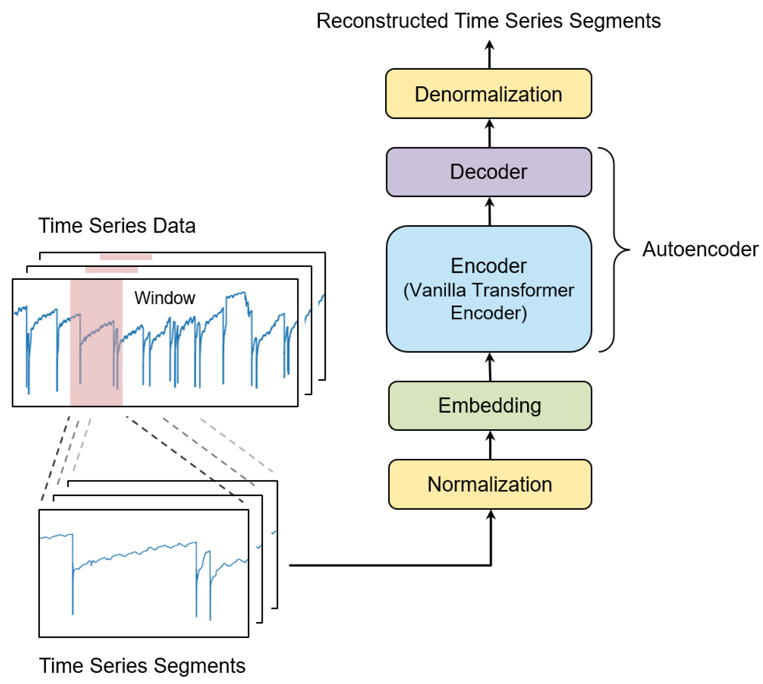
Figure 2.
Hyperparameter sensitivity analysis results of seven key hyperparameters for our proposed framework on four multivariate datasets. The hyperparameters are training window step size, window length, the number of attention heads, model dimension size, the number of encoding blocks, learning rate, and dropout.
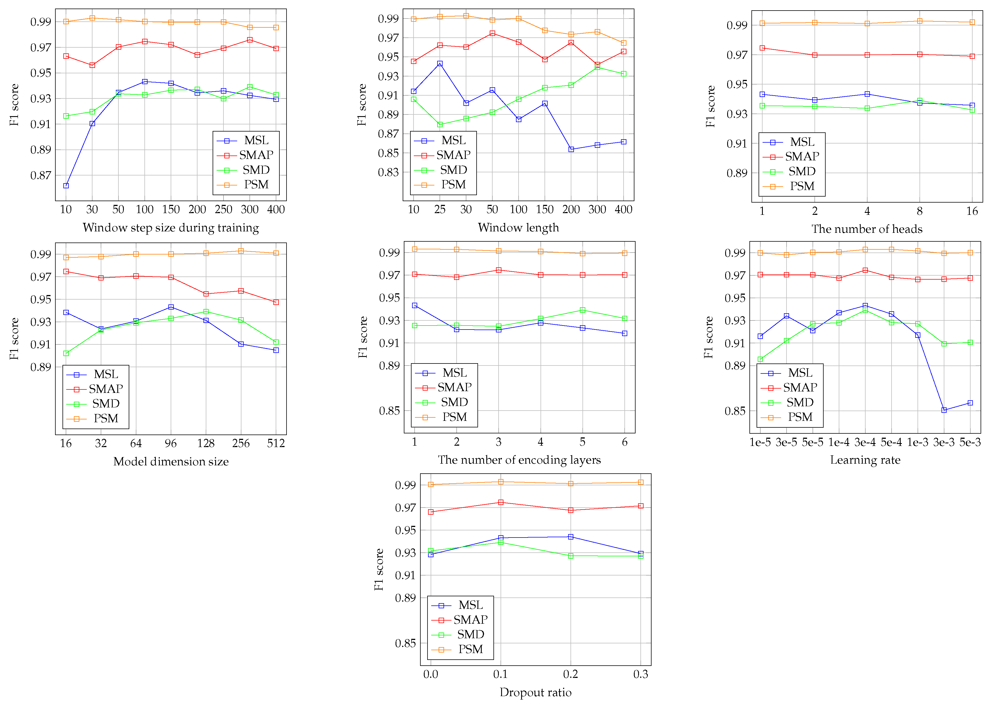
Table 3.
F1 score results on the six multivariate datasets. bold indicates the best performance, and underlined denotes the second-best.
Table 3.
F1 score results on the six multivariate datasets. bold indicates the best performance, and underlined denotes the second-best.
| MSL | SMAP | SMD | PSM | GECCO | SWAN-SF | |
| Anomaly Transformer | 0.936 | 0.967 | 0.923 | 0.979 | - | - |
| DCdetector | 0.966 | 0.970 | 0.872 | 0.979 | 0.466 | 0.734 |
| MEMTO | 0.944 | 0.966 | 0.935 | 0.983 | - | - |
| AnomalyLLM | 0.956 | 0.965 | 0.958 | 0.997 | 0.620 | 0.804 |
| Ours | 0.943 | 0.975 | 0.939 | 0.993 | 0.920 | 0.801 |
Table 4.
Affiliation F1 score results on nine univariate datasets.
| ABP | Acceleration | Air Temperature | ECG | EPG | |
| TS-TCC | 0.754 | 0.549 | 0.969 | 0.784 | 0.931 |
| THOC | 0.815 | 0.776 | 0.971 | 0.760 | 0.908 |
| NCAD | 0.794 | 0.849 | 0.758 | 0.735 | 0.789 |
| AnomalyLLM | 0.920 | 0.956 | 0.974 | 0.787 | 0.933 |
| Ours | 0.838 | 0.966 | 0.972 | 0.802 | 0.840 |
| Gait | NASA | Power Demand | RESP | Average | |
| TS-TCC | 0.794 | 0.511 | 0.763 | 0.560 | 0.735 |
| THOC | 0.784 | 0.896 | 0.775 | 0.389 | 0.786 |
| NCAD | 0.858 | 0.861 | 0.723 | 0.613 | 0.776 |
| AnomalyLLM | 0.871 | 0.961 | 0.886 | 0.736 | 0.892 |
| Ours | 0.867 | 0.926 | 0.865 | 0.763 | 0.871 |
Table 5.
Ablation analysis results of segment-level normalization-denormalization and positional encoding on three multivariate datasets. SegND represents segment-level normalization-denormalization, APE represents absolute positional encoding, and numbers in the cells represent F1 scores. ✗ signifies that the corresponding one is not used, while ✓ indicates that the corresponding one is used.
| SegND | Positional Encoding | MSL | SMAP | SMD |
| ✗ | ✗ | 0.909 | 0.740 | 0.830 |
| ✗ | APE (sinusoid) | 0.846 | 0.734 | 0.794 |
| ✗ | APE (learnable) | 0.902 | 0.710 | 0.845 |
| ✓ | ✗ | 0.943 | 0.975 | 0.939 |
| ✓ | APE (sinusoid) | 0.914 | 0.966 | 0.904 |
| ✓ | APE (learnable) | 0.924 | 0.957 | 0.923 |
Table 6.
Ablation analysis results of segment-level normalization-denormalization and positional encoding on three univariate datsets. SegND, APE, ✗ and ✓are described in Table 5. The numbers in the cells represent affiliation F1 scores.
Table 6.
Ablation analysis results of segment-level normalization-denormalization and positional encoding on three univariate datsets. SegND, APE, ✗ and ✓are described in Table 5. The numbers in the cells represent affiliation F1 scores.
| SegND | Positional Encoding | ECG | Gait | RESP |
| ✗ | ✗ | 0.739 | 0.783 | 0.693 |
| ✗ | APE (sinusoid) | 0.772 | 0.768 | 0.702 |
| ✗ | APE (learnable) | 0.746 | 0.819 | 0.703 |
| ✓ | ✗ | 0.802 | 0.867 | 0.763 |
| ✓ | APE (sinusoid) | 0.752 | 0.820 | 0.729 |
| ✓ | APE (learnable) | 0.759 | 0.850 | 0.721 |
Table 7.
Ablation analysis results of preprocessing time series data on three multivariate datasets, each comprising multiple sub-datasets (see Table 1). Sub-Dataset-Level refers to a case where a normalization method is applied to each sub-dataset within a dataset, while Dataset-Level refers to a case where a normalization method is applied to a single dataset that concatenates all its sub-datasets. The numbers in the cells represent F1 score results. ✗ signifies that the corresponding one is not used, while ✓ indicates that the corresponding one is used.
| Sub-Dataset-Level | Dataset-Level | MSL | SMAP | SMD |
| ✗ | ✗ | 0.943 | 0.975 | 0.939 |
| ✗ | min-max | 0.919 | 0.925 | 0.931 |
| ✗ | z-score | 0.887 | 0.707 | 0.877 |
| min-max | ✗ | 0.611 | 0.842 | 0.812 |
| min-max | min-max | 0.605 | 0.830 | 0.807 |
| min-max | z-score | 0.750 | 0.640 | 0.740 |
| z-score | ✗ | 0.923 | 0.692 | 0.811 |
| z-score | min-max | 0.922 | 0.823 | 0.808 |
| z-score | z-score | 0.887 | 0.655 | 0.799 |
Table 8.
Ablation analysis results of preprocessing time series data on four univariate datasets, each comprising multiple sub-datasets (see Table 2). Sub-Dataset-Level and Dataset-Level are described in Table 7. The numbers in the cells represent affiliation F1 scores. ✗ signifies that the corresponding one is not used, while ✓ indicates that the corresponding one is used.
| Sub-Dataset-Level | Dataset-Level | ECG | EPG | Gait | NASA |
| ✗ | ✗ | 0.672 | 0.840 | 0.725 | 0.926 |
| ✗ | min-max | 0.657 | 0.829 | 0.709 | 0.872 |
| ✗ | z-score | 0.670 | 0.812 | 0.712 | 0.892 |
| min-max | ✗ | 0.792 | 0.723 | 0.867 | 0.846 |
| min-max | min-max | 0.779 | 0.726 | 0.850 | 0.862 |
| min-max | z-score | 0.802 | 0.707 | 0.857 | 0.850 |
| z-score | ✗ | 0.735 | 0.667 | 0.825 | 0.914 |
| z-score | min-max | 0.756 | 0.677 | 0.815 | 0.883 |
| z-score | z-score | 0.764 | 0.711 | 0.831 | 0.870 |
Disclaimer/Publisher’s Note: The statements, opinions and data contained in all publications are solely those of the individual author(s) and contributor(s) and not of MDPI and/or the editor(s). MDPI and/or the editor(s) disclaim responsibility for any injury to people or property resulting from any ideas, methods, instructions or products referred to in the content. |
© 2025 by the authors. Licensee MDPI, Basel, Switzerland. This article is an open access article distributed under the terms and conditions of the Creative Commons Attribution (CC BY) license (http://creativecommons.org/licenses/by/4.0/).
Copyright: This open access article is published under a Creative Commons CC BY 4.0 license, which permit the free download, distribution, and reuse, provided that the author and preprint are cited in any reuse.


