Submitted:
08 January 2025
Posted:
08 January 2025
You are already at the latest version
Abstract
Aiming at the state estimation problem of non-linear systems (NLSs), the traditional typical nonlinear filtering methods (e.g., Particle Filter, PF) have large errors in system state, resulting in low accuracy and high computational speed. To perfect the imperfections, a new Bayesian estimation method based on particle flow velocity (PFV-BEM) is proposed in this paper. Firstly, the state update is carried out according to the projection principle to calculate the prior information of the state and select its particle points. Secondly, the particle flow velocity defined, which describes the evolution process of random samples from the prior distribution to the posterior distribution. The posterior information of the state is calculated by solving the parameters related the particle flow velocity. Finally, the estimated mean and standard deviation of the state are solved. Simulation experiments use one-dimensional general nonlinear examples and multi-target motion tracking as examples, it is compared with PF, the simulation results show the feasibility of the novel Bayesian estimation algorithm.
Keywords:
particle flow velocity
; non-linear systems
; Bayesian estimation
; probability density function
; Fokker–Planck equation
1. Introduction
In recent years, numerous mathematical models of engineering systems have exhibited strong nonlinear characteristics, which has rendered traditional Kalman Filter (KF) methods relying on linear assumptions ineffective when dealing with state estimation problems [1,2,3]. To address this challenge, academia has conducted in-depth research into nonlinear filtering techniques. Among these studies, the Extended Kalman Filter (EKF) emerged as an early solution, which linearizes nonlinear systems through Taylor series expansion and then applies the KF algorithm [4]. However, truncation errors introduced during the linearization process limit the accuracy of state estimation.
To overcome this limitation, Julier, Uhlmann, and others proposed the Unscented Kalman Filter (UKF) [5]. UKF avoids errors resulting from linearization by selecting a specific set of sample points to approximate nonlinear transformations, significantly improving the accuracy of state estimation.
Recently, Bayesian-based nonlinear filtering methods have become a research hotspot [6,7,8,9,10,11,12,13,14]. These methods are mainly divided into two categories: one approximates the state distribution in state space, with Particle Filter (PF) being one of the most representative algorithms [15]. PF represents the required posterior probability density through a weighted sum of random samples to estimate the state. Although PF theoretically approximates optimal Bayesian estimation, it still faces challenges in terms of estimation accuracy, implementation difficulty, and computational complexity in practical applications [16,17,18,19,20]. The other category directly approximates the state probability density function in function space. For example, the nonlinear projection filter algorithm proposed by Randal Beard and John Kenney addresses state estimation problems for low-dimensional nonlinear Gaussian systems [21,22,23]. Subsequently, scholars such as Zhao Yuxin proposed projection filter algorithms for one-dimensional nonlinear non-Gaussian systems, greatly reducing computational time complexity and memory usage [3].
It is worth noting that both EKF and UKF aim to solve for the second-order moments of the system state probability distribution, but the actual distribution of the system state may not be normal. Therefore, Bayesian estimation methods have advantages in non-Gaussian nonlinear systems, as they can directly solve for the system state probability density function, better capturing possible abrupt changes in the target state [16,17,18,19,20].
Literature [23] introduced a projection filtering method limited to low-dimensional state estimation problems. To overcome this limitation, this paper proposes a new Bayesian estimation method based on particle flow velocity(PFV-BEM)and extends it to nonlinear systems. Through numerical approximation solutions, simulation results demonstrate that this method not only relaxes the restrictive condition that system noise must be Gaussian but also outperforms PF algorithms in estimation accuracy and has lower computational complexity than general particle filters. Additionally, this method exhibits stable performance and has certain practical application value.
This paper is organized as follows. In Section 2, an Bayesian Estimation Model in NLSs is given, and the Bayesian equation of Bayesian Estimation Model is given. In Section 3, the (PFV-BEM) program is divided into two parts to solve the state solution: solving the prior probability for status update and using particle flow velocity for measurement update. In Section 4, two illustrative examples and their simulation results are given. Then, the conclusions of this paper are analyzed in detail In Section 5.
2. Bayesian Estimation Model
In nonlinear systems, the state estimation model consists of state equation and measurement equation, formulated as follows [24]:
where: denotes the state vector at time t, is the state transition matrix, represents the system noise driving matrix, is the standard Brownian motion and represents measurement noise, respectively, with denoting the measurement vector, and being the measurement matrix. and are mutually independent and satisfy:
where: is given as the system noise covariance matrix; represents the measurement noise covariance matrix.
According to a theorem in reference [25], the probability density function(PDF)of the state equation satisfies the Fokker-Planck Equation (FPE):
Where is defined as prior probability density.
the likelihood probability density of the measurement equation is defined as:
In reference [17], the state estimate solution of Bayesian estimation models needs to calculate the probability density function , which is defined as the posterior PDF of Bayesian Estimation Model. the posterior PDF satisfies Bayesian equation:
3. Bayesian Filter Estimator Design-Based Projection Flow Velocity
Bayesian estimation method based on particle flow velocity(PFV-BEM) is a state estimation method that approximates the PDF of the state. First, in the projection space, the prior PDF of the state can be calculated in its projection space. Second, the particle points of the prior PDF are obtained, through calculating the particle flow velocity, the particle information of the posterior PDF can be obtained, finally, the estimated solution and estimated variance of the system state can be calculated. Therefore, PFV-EMD is an effective method for solving Bayesian estimation problems. The flowchart of the PFV-BEM algorithm is shown in Figure 1.
3.1. Solving the Prior Probability for State Updates
State vector of state estimation model is given as , the PDF can be denoted as , , assume that the PDF of x can be expressed as the following form in reference [24]
where denotes standard orthogonal basis function in projection subspace, can be denoted as the coefficients of in Eq. (1), we definite , denotes the inner- product equation.
where denotes a complete set of basis functions for . could be denoted as the following form:
where coefficients is denoted as .These basis functions are given as:
where .
Simplify the above equation , ,
Simplify the Eq.(8), .
In reference [24],basic functionsis were given, According to solve the coefficients matrix , the PDF solution of can be solved.
Substitute Eq. (7) into Eq. (3), Eq. (3) can be rewritten as
Projecting Eq.(9) onto the project space , Eq. (9) can be rewritten as
If , and are given in Eq. (1) and Eq. (2). so Eq. (11) can be rewritten as
Simplify the Eq.(12), we defined
Eq. (12) can be rewritten as
where , is the element of matrix in Equation (14).
When , Eq. (12) can be rewritten as
Eq. (15) can be rewritten as
Set initial time ,the initial information , the initial coefficients of PDF can be given
Substitute Eq. (19) into Eq. (16), can be obtained:
If , Eqs. (20) have the following simple solution
priori coefficients can be given:
where are posterior coefficients of state at the time .
A priori PDF of state is given as
3.2. Using Particle Flow Velocity for Measurement Update
Randomly extract particle points based on the prior PDF at time . The posterior PDF of the state estimation model at time can be obtained by Bayesian formula Eq. (4). Homotopy function is expressed as:
where is the conditional PDF, represents the prior PDF, and represents the likelihood PDF.
Taking the logarithm of the above equation yields:
In the equation, is the normalization constant independent of x. Let λ change continuously from 0 to 1, and the homotopy function defines the probability distribution of the change from the prior distribution () to the posterior distribution (). The flow velocity of the state particle x during this process is described as the following differential equation.
The particle flow velocity satisfies FPE, which is the process noise. It can be obtained that:
Simplify the above equation:
Substituting equation (25) into equation (28) yields:
Simplify the above equation
The particle flow velocity field can be obtained as follows:
The variance is:
By using the velocity field calculation equation (31), the numerical integration of the prior particles with the posterior particles can be obtained as follows:
The estimated value of the state can be denoted as:
4. Illustrative Simulations Examples and Analysis
4.1. Example 1 and Analysis
For the first simulation example, In reference [26] considered a scalar signal process is observed through a scalar measurement process , and the NLSs model is given as.
where β(t) and η(t) are standard Brownian motions, and Initial state x(0) = 0, y(0) = 0.
The simulation time is T=2 seconds, and the number of particles is 1000. The estimate results are shown in Figure 2 and Figure 3. The priori PDF and posterior PDFs are plotted in Figure 2. The normalized density functions are plotted every other 0.1s. The partial results have been shown in Figure 2, where the actual position information (represented by black stars), PF estimated position information (represented by green squares), and PFV-BEM estimated position information (represented by red circles) are all displayed in Figure 2. The approximate particle flow in the PDF of the state is shown through the four graphs in Figure 2. Figure 3 provides a comparison chart of the estimated mean and variance of the two algorithms, where the PF estimation error is represented by a green line and the PFV-BEM estimation error is marked by a red line.
Figure 2a–d showcase partial estimation results of both particle filtering (PF) and the filtering algorithm proposed in this paper, along with the evolution of particles over time t. From Figure 2, it is evident that, in comparison to the PF algorithm, the proposed algorithm exhibits higher estimation accuracy, faster convergence speed, enhanced precision, and stable performance in system state estimation. The simulation results clearly demonstrate its capability to track the system state effectively. The feasibility of the proposed algorithm has been validated, making it apparent that PFV-BEM stands as an effective Bayesian estimation method for addressing state estimation problems in one-dimensional nonlinear systems.
4.2. Example 2 and Analysis
The continuous time stochastic differential equation interpretation of the dynamic tracking model is given by reference [27], which is described as follows:
State vector is defined as:
Measurement vector is defined as:
state estimation model is given as: .
the measurement model is denoted as
where: are respectively described as process noise of state equation and measurement noise of measurement equation, the covariance matrix respectively are and .State Transition Matrix is given as
Set the number of targets is 4, time steps are 400s, filter sampling time interval , running time T=400s, the number of particles is 2000.
For the three non-linear filtering methods of PF and PFV-BEM. The state estimation results based on PF and PFV-BEM are shown in Figure 4, Figure 5, Figure 6 and Figure 7. Figure 4 displays the state estimation results for four targets based on PFV-BEM, including comparisons between the true position information of the four targets and the position estimates obtained using the proposed algorithm, as well as comparisons between the true velocity information of the four targets and the velocity estimates derived from the proposed algorithm. Figure 5 presents a comparison of the position estimates for the four targets using PF and PFV-BEM. Additionally, Figure 5 also shows a comparison of the velocity estimates for the four targets based on PF and PFV-BEM. Figure 6 demonstrates the position and velocity estimation errors for the four targets tracked by the two algorithms. Figure 7 provides a comparison chart of the estimated mean of the two algorithms, where the PF estimation error is represented by a blue line and the PFV-BEM estimation error is marked by a orange line.
The figure presents partial estimation results obtained using particle filtering (PF) and the filtering algorithm proposed in this paper. As observed in Figure 4, the algorithm proposed in this paper demonstrates high estimation accuracy and provides precise estimation results in system state estimation. The simulation results indicate that PFV-BEM can effectively track changes in the system state. This verifies the feasibility of the algorithm. Evidently, for high-dimensional nonlinear systems, PFV-BEM serves as an effective Bayesian estimation method for solving the problem of state estimation in nonlinear systems.
5. Conclusions
This article validates one of the effective algorithms of PFV-BEM in Bayesian estimation methods. The basic core of its algorithm is that the filter estimator accurately calculates the prior and posterior probability density functions (PDF) through Bayesian iteration, and then estimates the mean and standard deviation of the system state. The article elaborates on the theoretical derivation in detail, mainly covering two aspects: obtaining prior PDFs through state updates and obtaining posterior PDFs through measurement updates. Through simulation experiments, the PFV-BEM filter outperforms the particle filter (PF) method in estimation accuracy. It has shown significant advantages in processing sensor data of complex nonlinear systems, especially in high-dimensional state estimation problems. It not only improves performance, but also accelerates computation speed and reduces computational complexity. Although the algorithm provides high-precision approximate solutions through time iteration, the selection of iteration time intervals is still challenging, and the convergence and robustness of the algorithm need further research. Therefore, we are committed to exploring more robust Bayesian estimation methods. These unresolved issues will become the focus of our future research.
Funding
Please add:This work has been supported by the National Natural Science Foundation of China (grant number52275266), Fundamental Research Funds for the Central Universities of China (grant number 410500078).
Conflicts of Interest
The authors declared that they have no conflicts of interest to this work. We declare that we do not have any commercial or associative interest that represents a conflict of interest in connection with the work submitted.
References
- Jun Shang, Tongwen Chen.Optimal stealthy integrity attacks on remote state estimation: The maximum utilization of historical data .automatic,Vol.128,2021. [CrossRef]
- Yuxin Zhao, Lijuan Chen,Yan Ma.An FEM-based State Estimation Approach to Nonlinear Hybrid Positioning Systems, Mathematical Problems in Engineering,Vol.2013,2013,pp.165-195. [CrossRef]
- Kalman, R. E., “A New Approach to Linear Filtering and Prediction Problems,” Transactions of the ASME. Journal of Basic Engineering, Vol. 82, No. 1, 1960, pp. 34-35.
- Kalman R. E., and Bucy, R. S., New Results in Linear Filtering and Prediction Theory, Transaction of the ASME, Journal of Basic Engineering, Vol. 83, 1961, pp.95-108.
- Rambabu Kandepu, Bjarne Foss, Lars Imsland, “Applying the unscented Kalman filter for nonlinear state estimation ,” Journal of Process Control, vol. 18(7-8), 2008., pp. 753-768. [CrossRef]
- Bucy R S,Senne K D. Digital synthesis of nonlinear filters. Automatica, vol.7,1971,pp.287-298. [CrossRef]
- Kushner, H. J., Dynamical Equations for Optimal Nonlinear Filter, Journal of Differential Equations, Vol. 3, No. 2, 1967, pp. 179-190. [CrossRef]
- Farhan A. Faruqi, Kenneth J. Tumer.Non-Linear Mathematical Model for Iniegrated Global Positioning/Inertial Navigation System.APPlied Mathematics and Computation. Vol.115,2000,pp. 213-227. [CrossRef]
- Julier, Simon, H.F Durrant-Whyte, “Process models for the high-speed navigation of road vehicles,” Proceedings - IEEE International Conference on Robotics and Automation, vol.1, 1995,pp.101 – 105. [CrossRef]
- Ann C.B.,William E.S..Bayesian Estimation of Multivariate Location Parameters,Handbook of Statistics.Vol.25,2005,pp. 221-244. [CrossRef]
- Nidhan C.,Subhashis G.,Anindy R.,William E.S..Bayesian Methods for Function Estimation,Handbook of Statistics.Vol.25,2005,pp. 373-414. [CrossRef]
- Sachin C.P.,Shankar N.,Prakash J.et.Nonlinear Bayesian state estimation: A review of recent developments,Control Engineering Practice.Vol.20,2012,pp.933-953. [CrossRef]
- Xu H.,Wen X. ,Yuan H. ,Duan K. , Liu W.,Wang Y. . fixed point iteration gaussian sum filtering estimator whith unknown time varying non gaussian measurement noise. Signal Processing, vol. 153,2018, pp. 132-142. [CrossRef]
- Y. Zhang, Z. Wu, N. Li, J. Chambers, A novel adaptive kalman filter with inaccurate process and measurement noise covariance matrices, IEEE Trans. Automat. Contr. vol. 63,no.2 ,2018,pp.594-601. [CrossRef]
- Park S.,P. Hwang J. , Kim E., Kang H.J. . A new evolutionary particle filter for the prevention of sample impoverishment, IEEE Transactions on Evolutionary Computation, vol. 13, No. 4,2009,pp. 801-809. [CrossRef]
- Gordon N.J., Salmond D.J., Smith A.F.M., “Novel approach to nonlinearnon-Gaussian Bayesian state estimation,” IEE Proceedings,Part F: Radar and Signal Processing, vol.140(2),1993,pp.107- 113. [CrossRef]
- Pitt M. K., Shephard N. Filtering Via Simulation: Auxiliary Particle Filters. Journal of the American Statistical Association,Vol.94, No.446,1999,pp. 590-591. [CrossRef]
- Rudolph van, der Merwe. The Unscented Particle Filte,2000,pp. 1-7.
- Kotecha J H, Djuric P M.Gaussian particle filtering. IEEE Transactions on Signal Processing,Vol.51(10),2003,pp.2592-2601. [CrossRef]
- Doucet and O. de Freitas, “Rao-Blackwellised particle filtering for dynamic bayesian networks; in Proceedings of the 16th Conference on Uncertainty in Artificial Intelligence, June 2000, pp.176-183.
- R. Beard, J. Gunther, projection filter based Guidance, Control and 1999. J. Lawton, and W Stirling, Nonlinear on galerkin approximation,Journal of Dynamics, vol. 22, no. 2, pp. 258-266. [CrossRef]
- Adel Hosseiny, Ghassem Jaberipur.Complex exponential functions: A high-precision hardware realization.Integration,vol. 73,2020,pp.18-29. [CrossRef]
- Saeed Hatamzadeh-Varmazyar, Zahra Masouri, Esmail Babolian,Numerical method for solving arbitrary linear differential equations using a set of orthogonal basis functions and operational matrix,Applied Mathematical Modelling,Vol. 40, Issue 1,2016,pp.233-253. [CrossRef]
- Lijuan Chen; Zihao Zhang; Yapeng Zhang; Xiaoshuang Xiong; Fei Fan; Shuangbao Ma ;Research on Projection Filtering Method Based on Projection Symmetric Interval and Its Application in Underwater Navigation, Symmetry, Vol.13no.9, 2021, pp. 1-19. [CrossRef]
- João M. Lemos, Bertinho A. Costa, Conceição Rocha,A Fokker-Planck approach to joint state-parameter estimation,IFAC-PapersOnLine,Volume 51, Issue 15,2018, pp. 389-394. [CrossRef]
- Benes, V. E. (1981). Exact finite-dimensional filters for certain diffusions with nonlinear drift. Stochastics, 5:65–92. [CrossRef]
- Julier, S. J. and Uhlmann, J. K. . Unscented filtering and nonlinear estimation. Proceedings of the IEEE, 92(3),2004,pp.401–422. [CrossRef]
Figure 1.
Flowchart of the estimator based on PFV-BEM.
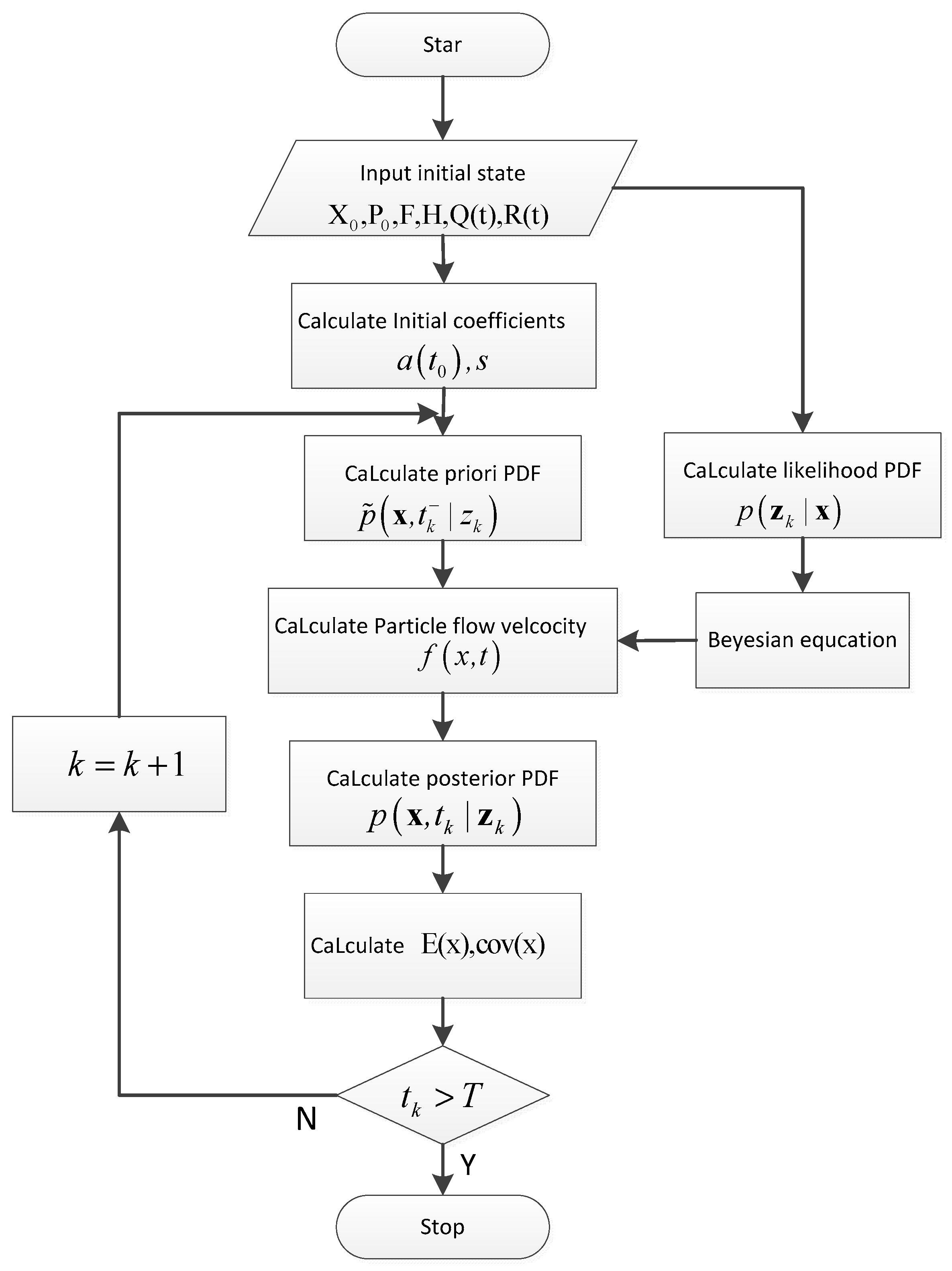
Figure 2.
Real location information, PF estimated location information, and PFV-BEM estimated location information during certain time periods (a) display state estimation information result at t=0.1s (b) display system state estimation information result at t=1s (c) display system state estimation information result at t=1.5s (d) display system state estimation information result at t=2s.
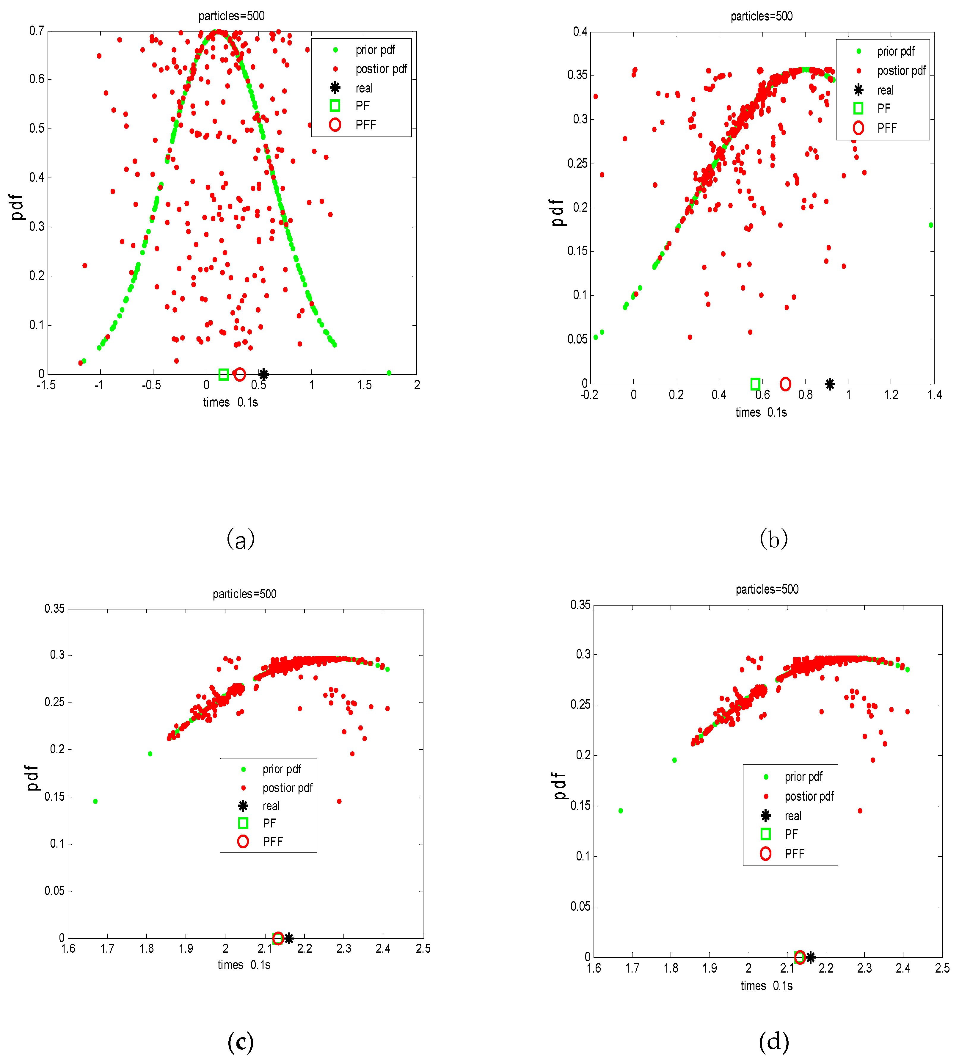
Figure 3.
Estimated mean and standard deviation of PF and PFV-BEM, they should be listed as: (a) The first section contains the comparison results of estimation errors between two algorithms; (b) The second section contains the comparison results of estimating mean square error using two algorithms.
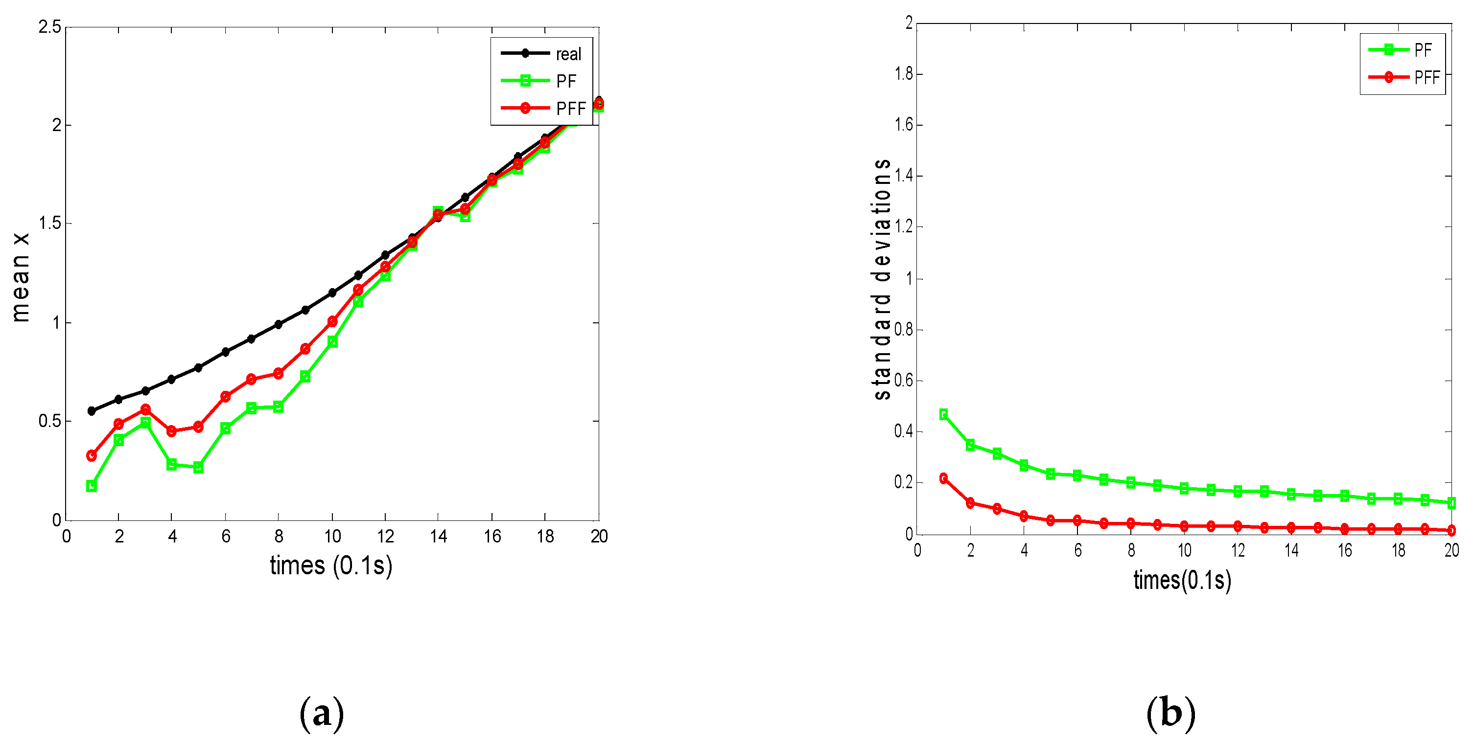
Figure 4.
The state estimation results of 4 targets based on PFV-BEM.
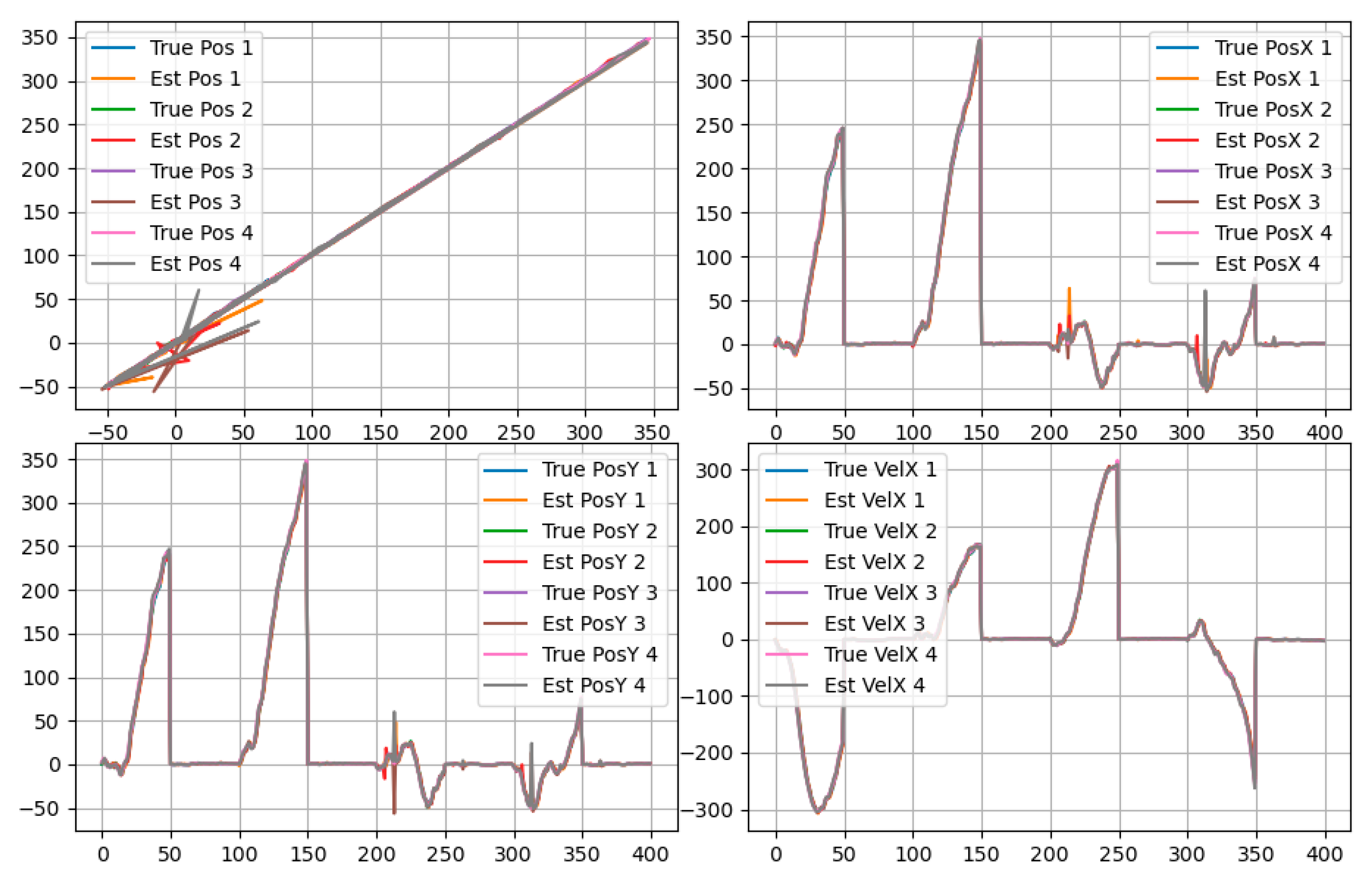
Figure 5.
The position estimation results of 4 targets based on PF and PFV-BEM.
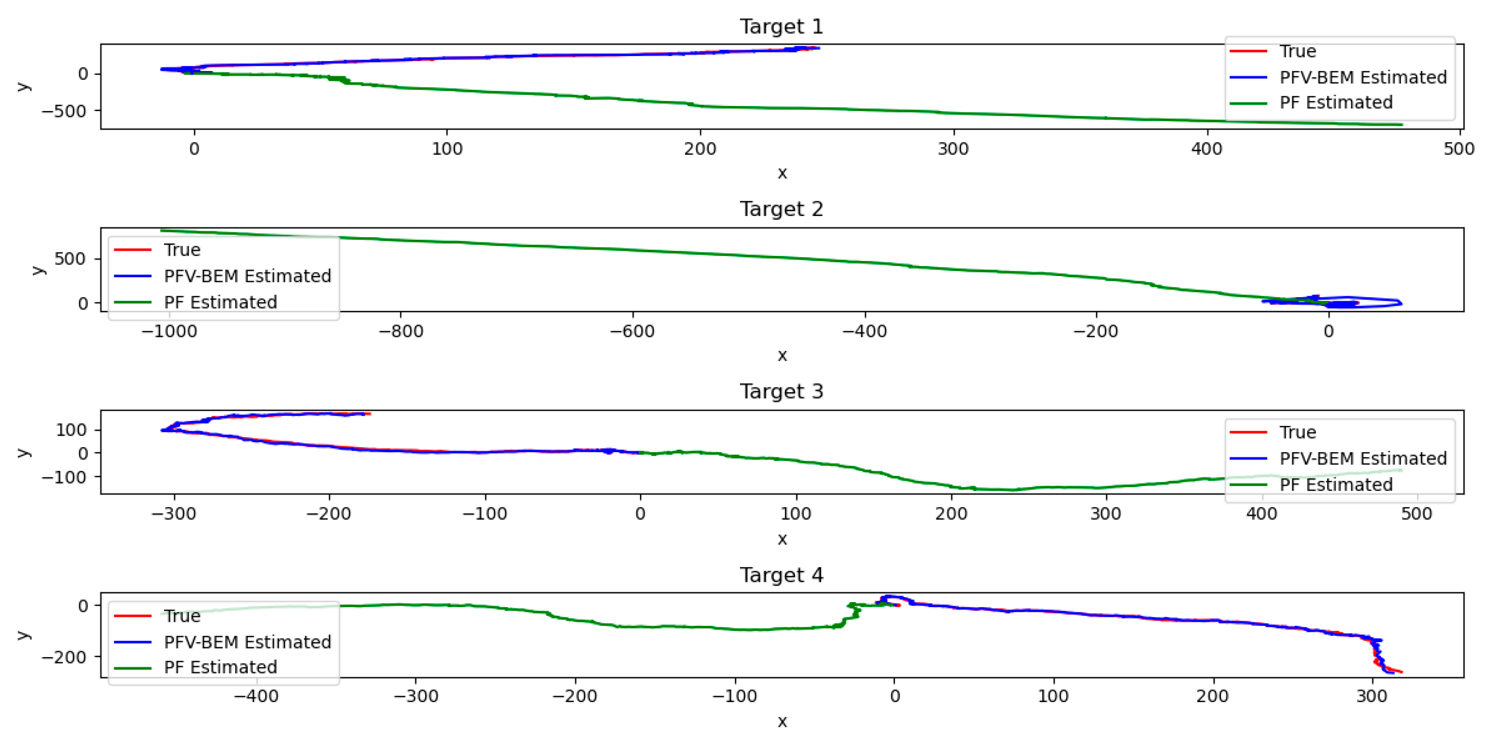
Figure 6.
The velocity estimation results of 4 targets based on PF and PFV-BEM.
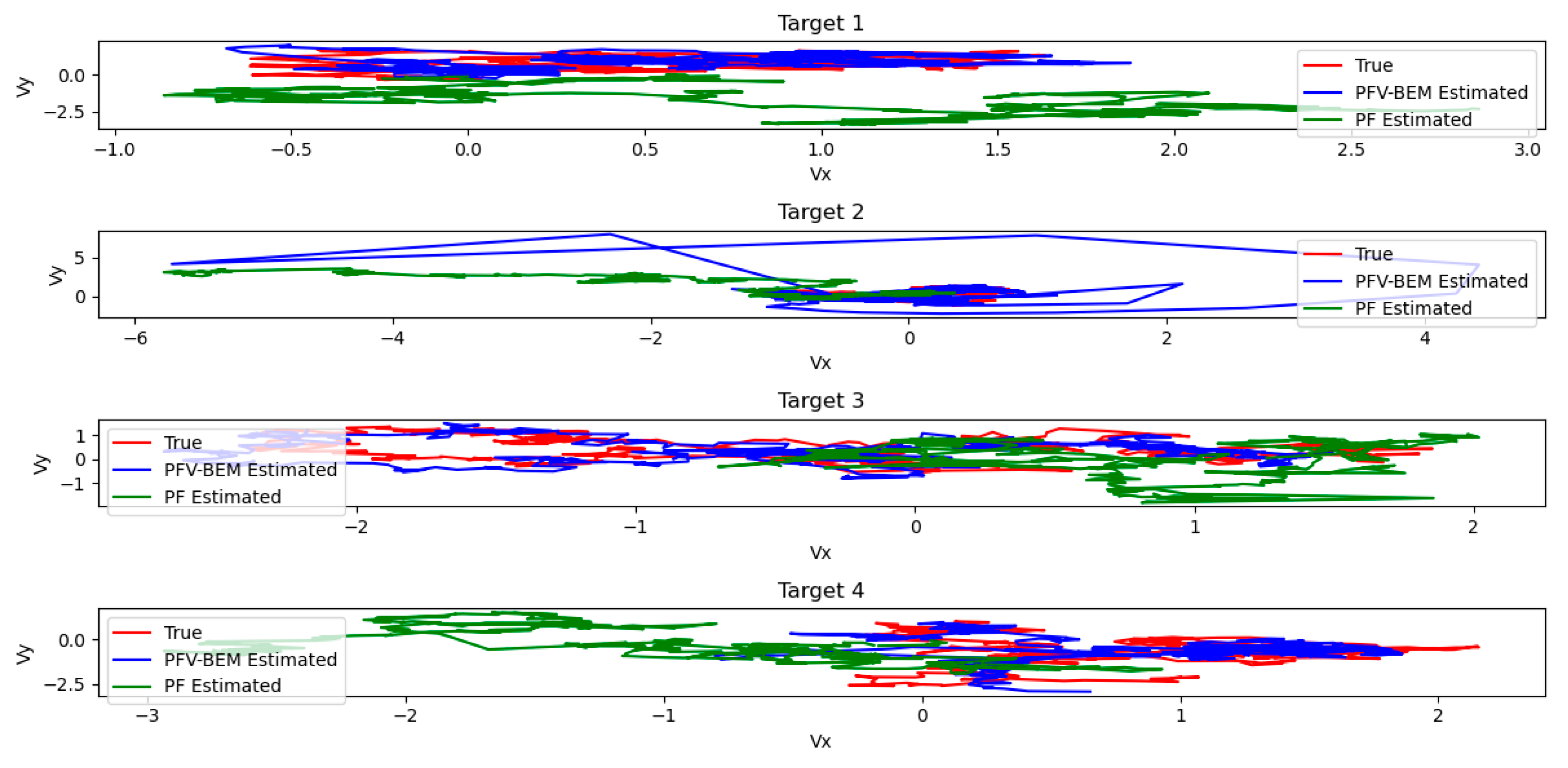
Figure 7.
The position and velocity estimation error results of 4 targets based on PF and PFV-BEM

Disclaimer/Publisher’s Note: The statements, opinions and data contained in all publications are solely those of the individual author(s) and contributor(s) and not of MDPI and/or the editor(s). MDPI and/or the editor(s) disclaim responsibility for any injury to people or property resulting from any ideas, methods, instructions or products referred to in the content. |
© 2025 by the authors. Licensee MDPI, Basel, Switzerland. This article is an open access article distributed under the terms and conditions of the Creative Commons Attribution (CC BY) license (http://creativecommons.org/licenses/by/4.0/).
Copyright: This open access article is published under a Creative Commons CC BY 4.0 license, which permit the free download, distribution, and reuse, provided that the author and preprint are cited in any reuse.


