
Submitted:
05 January 2025
Posted:
06 January 2025
You are already at the latest version
Abstract
This paper introduces a novel method for comparing three dimensional point clouds, a critical task in various applications such as computer vision, pattern recognition etc. In this method, point cloud is interpreted as samples from an underlying probability distribution-Gaussian Mixture Model. Then, a rigorous mathematical foundation is established by proving that the space of Gaussian Mixture Models form a statistical manifold. The statistical manifold structure of Gaussian Mixture Model enables us to use the information geometric tools for similarity measure. The similarity or distance measures between Gaussian Mixture Models plays a crucial role in many applications. In this paper, the Modified Symmetric Kullback-Leibler Divergence is used for the similarity measure. This method of comparing the point clouds takes care of the geometry of the objects represented by the point clouds. The experimental result on comparison (i) of basic geometric shapes, (ii) of three-dimensional human body shapes within a comprehensive human body shape dataset, (iii) of animal shapes and (iv) of point clouds of same objects produced from the dense point clouds in Point Cloud Upsampling Adversarial Network dataset indicate that the information geometric method achieves superior performance compared with the state-of-the-art methods and valuable insights are derived from the results.
Keywords:
Information Geometry
; Gaussian Mixture Model
; Statistical Manifold
; Divergence
; Point Cloud
1. Introduction
Three-dimensional point cloud is a highly accurate digital record of an object. Point clouds provide a flexible geometric representation suitable for applications in computer graphics, photogrammetry, computer vision, the construction industry, remote sensing, etc. The extraction of meaningful information from point clouds is fundamental for many applications. In particular, applications such as registration, retrieval, and autoencoding require comparison of point clouds. Comparing point clouds is challenging due to their inherent properties and the geometry of underlying surfaces they represent. Unlike structured data on grid, point clouds do not have a common metric, such as the Euclidean metric. Because of this, direct comparisons between point clouds are difficult. When comparing point clouds which are sampled from 3D surface, the primary goal is to compare the overall surface and not the specific points.
The aim of this work is to develop a theoretical and computational framework for point cloud analysis using information geometric tools that take care of the shape, structure, pattern, and overall distribution. First, using the deep learning models such as DGCNN (Dynamic Graph Convolutional Neural Network) and FCNN (Fully Connected Neural Network) [13] followed by the Gaussian Mixture Model (GMM) the probability density function governing the point cloud is obtained. Then, consider the set S of all probability density functionns - the statistical model - representing the space Z of point clouds. Further a rigorous mathematical foundation is established by proving that the statistical model S representing the space Z of point clouds is a statistical manifold. Now, information geometric tools on the statistical manifold can be used for similarity measures. In fact, one can use any suitable diveregence for similarity measure. In this paper, Modified Symmetric Kullback-Leibler(MSKL) Divergence is used for measuring the similarity of point clouds. The proposed information geometric method provides a better understanding of point cloud similarity, considering their geometric properties and effectively handles complex data through information geometric techniques. The information geometric framework introduces a novel approach in comparison of point clouds that captures both local and global geometric properties and statistical relationship. Rich intrinsic geometric properties can be obtained using this method.
To demonstrate the effectiveness of our approach, we present four case studies (i) comparison of basic geometric shapes, (ii) comparison of 3D human body shapes within the MPI FAUST dataset in (a) same shape recognition (b) same person in different postures (c) point clouds of same person with different coordinates, (iii) comparison of animal shapes, and (iv) Comparison of different down-sampled point clouds of same objects (sculptural models of a boy) produced from the dense point clouds in PU-GAN dataset.
The comprehensive experimental validation across multiple datasets demonstrates the method’s effectiveness. For basic geometric shapes (cube, cone, sphere), information geometric method shows enhanced sensitivity to shape variations while maintaining accuracy in identical shape recognition. In the MPI FAUST dataset, the framework successfully handles human body shapes across different postures and coordinate systems, demonstrating invariance to rigid transformations. With animal shapes from the G-PCD dataset, our approach effectively distinguishes between complex morphological features while maintaining shape identity. In the PU-GAN dataset comparisons, information geometric method proves robust across different complex (sculptural) shapes, effectively capturing geometric details at various scales.
2. Related Works
A significant part of working with point clouds involves comparing them to assess similarity. The Hausdorff distance [2], Chamfer distance [3], and Earth mover’s distance [5] measures are commonly employed. However, these measures focus primarily on how close the points are to each other, which may fail to consider the broader context and thus the overall shape and structure of the point clouds. This limit their effectiveness in capturing the intrinsic geometric properties essential for accurate comparison.
The Hausdorff distance is an important metric in areas such as computer vision, pattern recognition, and 3D shape analysis. It is particularly useful in highlighting the dissimilarity between two point sets and is defined for two finite point sets P and Q as
This measure emphasizes the largest difference between two sets of 3D points, which makes it particularly sensitive to unusual points that do not fit in the pattern.
Our method leverages information geometry to mitigate the issue of unusual points by focusing on the underlying statistical properties of point clouds. By treating point clouds as samples from underlying probability distributions, we enable a comprehensive evaluation that incorporates both spatial and statistical relationships, offering a robust comparison technique.
The Chamfer distance provides an alternative that averages point-to-point distances, thereby reducing the impact of outliers. It is widely used in 3D reconstruction and mesh generation.
This method calculates the average of the squared distances between each point in one set to its nearest point in the other set, offering a balance between sensitivity to large discrepancies and outliers. In this method differences in point cloud shape and distribution is not taken care of.
By integrating geometric tools with probabilistic analysis, our method provides a nuanced assessment of point cloud similarity. Information geometric techniques enable the detection of subtle differences in point cloud shape and distribution, offering advantages in complex scenarios where context and relationships of 3D points significantly influence data structure and interpretation.
Another method for comparing the similarity and dissimilarity between point clouds is the Earth Mover’s Distance (EMD),
Here, denotes the bijection between point clouds A and B. Although EMD is insightful for measuring the dissimilarity by conceptualizing the minimum cost of transforming one point cloud into another, it might not take into account the overall shape and intrinsic geometric structures of the point clouds. This limitation can lead to a less comprehensive understanding of point cloud similarities and differences, especially in contexts where the geometric and topological properties are of significant importance [5].
Our approach addresses this limitation by incorporating both geometric and probabilistic properties of point clouds into the comparison. By doing so, it allows for a deeper analysis of the point clouds’ intrinsic structures, making our method highly effective in applications where the data’s geometric and statistical characteristics are crucial. This provides a more robust comparison mechanism, especially beneficial in scenarios where understanding the complex interplay between shape, structure, and distribution is paramount.
In [2] and [3]comparing two objects reduced to the comparison between the corresponding interpoint distance matrices in the multidimensional scaling. In these methods, information about rigid similarity is only attained. But for isometric objects, allowing bend and not just rigid transformation Facundo Mémoli and Guillermo Sapiro developed a method in [4]. The underlying theory in the isometric invariant recognition is based on the Gromov-Hausdorff distance. This theory is embedded in a probabilistic setting by points sampled uniformly and using the metric as pairwise geodesic distance.
where
and are subsets of the manifold Z with the intrinsic geodesic distance function . Since there is no efficient way to directly compute the Gromov-Hausdorff distance they introduced a metric
where is the set of all permutations of , n is the number of points in the point cloud. This metric satisfies . The metric is computable and can be used to replace .
The framework for comparing point clouds developed in [4] may face challenges with highly complex or high-dimensional geometric structures due to computational constraints. In this method, geodesic distances are approximated using techniques like the isomap algorithm, which relies on constructing a neighborhood graph from the nearest neighbors. While effective for simpler datasets, this approach can become computationally intensive for highly complex data, where the intrinsic geometric structures demand more nuanced distance calculations to accurately capture the manifold’s topology.
In the information geometric method the point clouds are represented by probability density functions and a statistical manifold structure is given to the space of point clouds. This statistical manifold structure enables a more comprehensive and robust comparison, as it considers both the spatial distribution and the statistical relationships between points.
3. Information Geometry
Information geometry explores the application of non-Euclidean geometry in probability theory in general and with a specific focus on it’s application in statistical inference and estimation theory. This approach has proved to be highly effective in many applications, such as neural network, machine learning, mathematical finance,control system theory, statistical mechanics etc. Metrics and divergences between probability distributions is important in practical applications to look at similarity/dissimilarity among the given set of samples [10,20].
The basis of a statistical model resides in a family of probability distributions, which are represented by a set of continuous parameters that constitute a parameter space. The local information contents and structures of the distributions induce certain geometrical properties on the parameter space. The pioneer work of Fisher in 1925, studying these geometrical properties, has received much attention. The introduction of Riemannian metric in terms the Fisher information matrix by C. R. Rao in 1945 [19] marked a significant milestone. This inspired many statisticians to study the geometric theory in the context of probability space.
Now, we give a brief account of the geometry of statistical manifolds [1,18]. For basic knowledge in differential geometry refer [6].
3.1. Statistical Manifold
Now, we describe the manifold structure and its geometry for a statistical model, this will be the foundation of information geometric approach to point clouds.
Let be a probability space, where . Consider a family of probability distributions on . Suppose each element of can be parametrized using n real-valued variables so that
where is an open subset of and the mapping is injective. The family is called an n-dimensional statistical model or aparametric model.
For a model , the mapping defined by allows us to consider as a coordinate system for . Suppose there is a diffeomorphism , where is an open subset of . Then, if we use instead of as our parameter, we obtain . This expresses the same family of probability distributions . If parametrizations which are diffeomorphic to each other is considered to be equivalent then is a differentiable manifold, called the statistical manifold.
3.2. Divergence Measures on Statistical Manifolds
Divergence is a distance-like measure between two points (probability density functions) on a statistical manifold. The divergence D on S is defined as a smooth function satisfying, for any
The KL divergence is defined as [8],
where and are probability density functions.
In general, divergences are not symmetric, in this paper, we are using the modified version of KL divergence called Modified Symmetric KL divergence, denoted as , defined as
4. Information Geometric Framework for Point Cloud Data
In this section, we establish a statistical manifold framework for point clouds dataset. Consider the dataset X with n points in , i.e , assuming that all the points are distinct. Denote the set of all point clouds by
4.1. Covering in the Context of Point Clouds
The concept of ’covering’ plays an important role in the study of point clouds within the framework of topological spaces. A covering in the context of point clouds refers to using a group of smaller sets to represent different parts of the whole point cloud.
A covering of X is defined as a finite collection of subsets of X, such that Each is a subset of X representing a localized region of the point cloud. The key properties to be satisfied by this covering are
- Locality: For each subset , there exists an open set containing in X. Mathematically, this can be represented as .
- Overlap: For any two distinct subsets and , their intersection is not necessarily empty, that is for some .
4.2. Statistical Manifold Representation
By choosing the finite subsets of the point cloud X, we are simplifying the point cloud X while still preserving its key features. This simplification is particularly important for finding the probability distribution governing this data using Gaussian Mixture Models (GMM). Then, the statistical manifold structure is given to the space Z of point clouds. By this, we obtain a manageable and accurate representation of the point clouds as a statistical manifold preserving the geometric nature of the object.
4.2.1. Gaussian Mixture Model
The fundamental idea to obtain the statistical manifold is to view a point cloud X as a collection of n samples originating from an underlying probability density function which is a point in the manifold. Using the Gaussian Mixture Model [7], a parametric probability density function is constructed for the point cloud data, where is the parameter set representing the GMM.
px
A Gaussian Mixture Model , in the context of point clouds, represents a composite distribution wherein each data point x in the point cloud X is assumed to be drawn from one of the K Gaussian components. The model is parametrized by the parameter set , where is the mean vector, is the covariance matrix, and is the mixing coefficient.
Mathematical Formulation:
- Gaussian Distributions: Each Gaussian component in the mixture is defined by its mean and covariance . The probability density function of a Gaussian is given bywhere x is a data point in the point cloud X, m is the dimensionality of the data, and is the determinant of the covariance matrix.
- Mixing Coefficients: These are denoted by for each Gaussian component and they satisfy
- Final Model: The probability density function of the entire mixture model for a data point x in the point cloud X is given byThis is the statistical representation of the point cloud X.
4.2.2. Manifold Structure for Point Clouds
Consider the space Z of point clouds, where each point cloud is represented as . Point cloud X has a statistical representation where the parameter varies over the parameter space . The set S of all the probability density functions representing the point clouds in the space Z is the statistical model representing Our aim is to give a geometric structure, called statistical manifold, to the space
Theorem 1.
Let and be two univariate Gaussian mixture models representing the point cloud X having the number of Gaussian components K and L respectively. Suppose that for all x in a set with no upper bound,
If the components are distinct and they are ordered lexicographically by variance and mean, then and for each i, , , and .
Proof.
Arrange the components of each GMM in increasing order of their variances. For we have , and for we have . If , then , and similarly if then .
For all x in a set with no upper bound,
Consider the component with the largest variance in each GMM. Without loss of generality, assume and are the largest variances in their respective GMMs. Then,
Since the two GMMs are equal for all x, their limits must also be equal. That means and . Then,
By repeating the above steps we conclude that and for each , the parameters are equal: , , and . □
Theorem 2.
The parameter space
for GMMs with K components of m-dimensional Gaussian is a topological manifold.
Proof.
For the probability density function
each is an dimensional vector. The diagonal covariance matrix is symmetric, thus having m distinct elements. The total number of mixing coefficients are K and since only are independent.
The parameter space T is
The total number of independent parameters in is
Note that , so is a topological space with standard Euclidean topology. Also, around any point in there exists a neighborhood that is homeomorphic to an open subset of . This satisfies the local Euclidean condition for a manifold. Therefore, the parameter space of Gaussian Mixture Models with K components of m-dimensional Gaussian is a topological manifold of dimension . □
Theorem 3.
The statistical model S representing the space Z of point clouds is a statistical manifold of dimension .
Proof.
Consider the map , defined by for . Now to show that it is injective under the condition that the covariance matrices are diagonal. Consider two GMMs with parameter sets
and
where and are diagonal matrices.
Assume for all x. By the Cramér-Wold theorem [9], this equality holds if and only if their projections onto any direction are equal.
For any direction ℓ, the property of multivariate normal distributions ensures that if , then
Therefore, projecting GMMs gives
These projected distributions are univariate GMMs, as each is scalar-valued and the mixture structure is preserved. By Theorem 1, the equality of these univariate GMMs for all directions ℓ implies
for all i and all ℓ.
Since this holds for all projection directions ℓ, we conclude that , proving that h is injective. The parameter space is a topological manifold and the mapping is injective hence the statistical model representing the space Z of point clouds can be viewed as a statistical manifold of dimension □
5. Data Overview and Preprocessing
This section is an overview of the data sources used in the study, including basic geometrical shapes, MPI FAUST dataset and PU-GAN dataset that are processed into point cloud representations. The preprocessing steps are designed to ensure that the data types are compatible with the computational framework.
5.1. Basic Geometrical Shapes
We consider three basic geometrical shapes in : unit cube , cone , and unit sphere , all centered at the origin.
U is defined by: . For each point the coordinates are generated using a uniform distribution over .
Each point in the cone C is represented by cylindrical coordinates , where is uniformly distributed over , h over and the radii . The angles are uniformly distributed over , the heights over , and the radii are calculated using . The cylindrical coordinates are then converted into cartesian coordinates using
For S, each point is represented by its spherical coordinates . The angles and are uniformly distributed over and respectively. The spherical coordinates are then converted into cartesian coordinates using
5.2. Human and Animal Dataset
For the human dataset, we employ the MPI FAUST dataset, a collection of high-resolution 3D scans of human figures in various poses. These point clouds capture the geometry of the human form, making them an invaluable resource for analyzing shape and structure within our geometric framework [14]. For the animal dataset, we utilize the G-PCD: Geometry Point Cloud Dataset, which has rich local geometrical information [15].
5.3. PU-GAN Dataset
The PU-GAN dataset [16] contains a diverse collection of 3D point cloud models ranging from basic geometric shapes to complex sculptures. This dataset is particularly valuable because it provides both sparse and dense point cloud representations of the same objects, making it ideal for evaluating different point cloud comparison methods. In this study, we use detailed sculptural forms (boy), which offer different levels of complexity for testing the performance of information geometric method.
6. Computational Foundation
In this section, the computational approach for comparing the point clouds is given. By using the deep learning techniques and EM algorithm we converted the point clouds into the probability density functions and given the statistical manifold structure to the space of point clouds. Now, we use the theory that developed in section 4 to analyze the similarities or dissimilarities between point clouds using information geometric techniques. In the information geometric method (IGM), the similarity of the probability density function is measured using divergence, we employ the MSKL divergence in this paper.
6.1. Sampling
Farthest Point Sampling (FPS) Method: The Farthest Point Sampling (FPS) [12] is used to choose the samples from the point clouds. FPS is chosen because of its effectiveness in preserving the geometric and topological properties of the datasets.
Consider two distinct point clouds, X and Y of dimension m. The FPS process involves,
- Initialization: Select an initial point randomly from the point cloud X. Set .
-
Iterative Selection: Choose the point that has maximum distance form . Now choose where , such that gives minimum value for .the sample set U is selected with the required number of points in this way.
- Sample Extraction: Using the above procedure choose 960 samples of 512 points each for both X and Y. Let the sample sets of X and Y be denoted by and .
6.2. Labeling and Data Splitting
In this section, the process of preparing the dataset from point clouds X and Y is given. Initially, we extracted 960 samples, each consisting of 512 points, from both the point clouds. These samples were then labeled distinctly, those from X as “First” and from Y as “Second.” This labeling was critical for identifying the source of each sample in subsequent analysis.
After the sampling combine the labeled samples into a single dataset, comprising 1920 samples in total. This dataset is then divided into training, validation, and testing sets in a 70%, 15%, and 15% split, respectively. This division was carefully executed to ensure an equal distribution of samples from both point clouds in each subset, maintaining the balance and integrity of the dataset for our analysis. This setup forms the foundational basis for the computational exploration and analysis that follows.
6.3. Model Implementation
In this section, the implementation details of the DGCNN-FCNN (Dynamic Graph CNN followed by a Fully Convolutional Neural Network), and encoder-decoder model are discussed. This model implementation is taken from [13], because of its proven effectiveness in similar contexts.
This model takes input point clouds of 3×512 dimension. These point clouds are passed through a series of five EdgeConv layers at the initial stage. These layers are unique in their pointwise latent space dimensions set at , and a max pooling layer. We do not use the batch normalization layer. The output of this DGCNN is 1024 dimensional feature vector. Other parameters , leaky ReLU activation function are same as the original DGCNN model. Further, this feature vector undergoes three fully connected neural networks with dimensions , with a leaky ReLU activation function and a linear output activation function. The resultant latent space is two-dimensional.
A key aspect of this approach is minimization of the reconstruction loss to ensure that the 2D latent space provides the most accurate representation of the original point cloud.
The same FCNN (fully connected neural network) is used for the decoder. The two dimensional vector from the latent space is passed through three fully connected neural networks with dimensions (256, 512, 3×512), with a ReLU activation function and a linear output activation function. The final output of this process is a reconstructed three dimensional point cloud with 512 points.
Training Details: To train our networks, we utilize the ADAM optimizer with a learning rate of 0.001. We use the Chamfer distance to compute the reconstruction loss. The training parameters, however, vary depending on the data type. For 3D Basic geometrical shapes, human body, and animal point cloud datasets, we conduct the training with a batch size of 16 and 400 epochs.
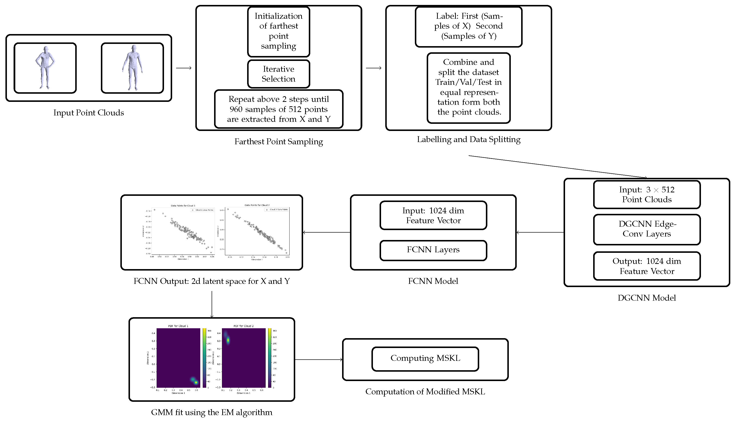
Figure 1.
Flowchart of the Computational Process.
6.4. Probability Density Function Estimation Using GMM
After the model training phase, we fit Gaussian Mixture Models (GMM) for estimating the probability density functions for the point cloud data.
After training the model, test data corresponding to the label “First” is given as input to the trained model. This will generate a 2D latent space. Then, input the data corresponding to the label “Second,” to generate another 2D latent space. The Gaussian mixture model is fit to each latent space using the Expectation-Maximization (EM) algorithm [17].
6.5. Space of Point Clouds as Statistical Manifold
After estimating the probability density functions for the point clouds using the Gaussian mixture model, we give the statistical manifold structure to the space of point clouds using the theory that we established in Theorems 1, 2, and 3 of section 4. This statistical manifold structure allows us to apply information geometric methods to compare and analyze the point clouds.
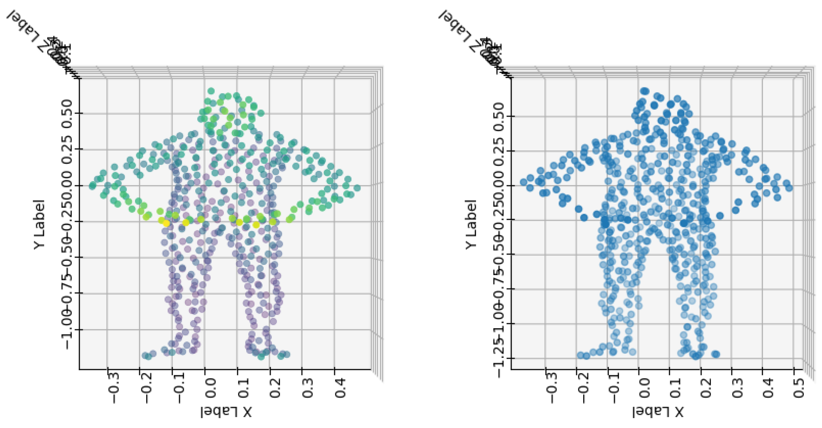
Figure 2.
Left: The original point cloud sample extracted using FPS. Right: Reconstructed point cloud sample after passing the encoder output to the decoder model.
Figure 2.
Left: The original point cloud sample extracted using FPS. Right: Reconstructed point cloud sample after passing the encoder output to the decoder model.
6.6. Modified Symmetric KL Divergence
After giving the statistical manifold structure to the space of point clouds we now use the Modified Symmetric KL (MSKL) divergence for measuring similarity and dissimilarity among the point clouds. Take two sets of samples and from two probability density functions and using a grid-based approach, instead of random sampling. This method involves creating a grid over the data range and calculating the PDF values at each grid point.
This sampling method evenly covers the entire sample area and accurately calculates the PDF values, whereas in the random sampling using Monte Carlo [11], it might be possible that the sampling does not cover the sample area accurately.
To handle regions where probability density might be zero, we add a small constant to the probability values before computing logarithms. The value of is chosen based on the nature of the dataset: for human body shapes (MPI FAUST), animal shapes (G-PCD), and sculptural shapes (PU-GAN) due to their complex geometric variations, while is used for basic geometric shapes where the probability distributions are more uniform. Then computed, for each in
and for each in .
The Modified Symmetric KL divergence,
is then computed.
7. Case Studies
The information geometric method is applied to four different cases and it is compared with other traditional measures . Each case demonstrates the effectiveness of the information geometric method for the point cloud comparison.
7.1. Comparision of Basic Geometrical Shapes
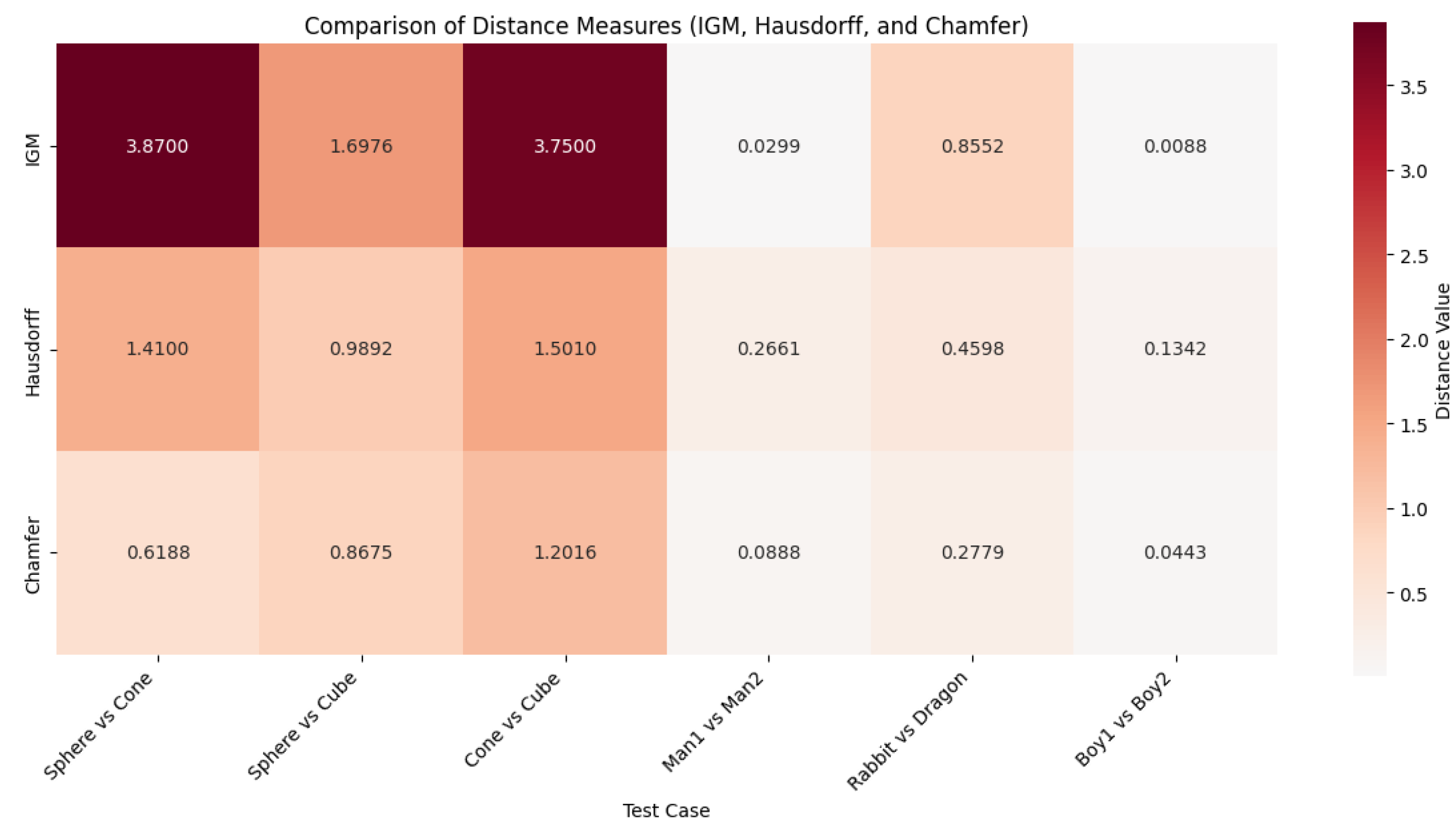
Now, we compare the basic geometric shapes using the information geometric method(IGM), Hausdorff distance(H) and Chamfer distance(Ch). This case study demonstrates the IGM’s effectiveness in distinguishing different geometric shapes compared to Hausdorff and Chamfer distances. Also, the IGM shows higher sensitivity to shape variations between the sphere, cone, and cube.(See Table 1).
7.2. Point Cloud Comparison of the Human Body
Accurate comparison of 3D human body shapes has significant implications in various computer vision and geometric analysis applications. The IGM shows a relatively small value when comparing the same person in different postures (Man1 vs. Man2) which indicate that it is more robust to posture changes while maintaining shape identity. The Hausdorff distance exhibits the highest value reflecting its sensitivity to outliers and maximum point-wise distances between the shapes. The Chamfer distance shows an intermediate value representing the average point-wise distances between the shapes (Table 2).
Netx, measure the similarity between two point clouds that describe the same object with different point distributions and scans, this is achieved by rotating one of the point cloud by 5 degree. The IGM (0.00324) demonstrate strong coordinate invariance with a minimal value indicating its robustness to different coordinate representations. The Hausdorff (0.04019) and chamfer (0.017) distance exhibits moderate sensitivity to coordinate change due to its point-wise computation (see Figure 3).
7.3. Point Cloud Comparison of Animals
The analysis of the animal dataset [15] demonstrates the effectiveness of different metrics in handling complex animal morphologies. The IGM effectively captures overall morphological differences in body structure, variations in surface curvature, and complex geometric patterns that define each animal’s unique shape compared to Hausdorff and Chamfer distance(see Table 3).
7.4. Point Cloud Analysis Using PU-GAN Dataset
In this section, the analysis of information geometric approach on PU-GAN dataset, a benchmark dataset widely used for point cloud processing and analysis, is given. We examine the sculptural model (boy) from this dataset, demonstrating the effectiveness of IGM for complex point cloud structures. The IGM effectively identifies the underlying similarities in the complex sculptural model, whereas Hausdorff and Chamfer distances are more sensitive to local variations. Thus IGM method is effective in the case of large number of dense and sparse point clouds (see Table 4).
Figure 4.
Comparison of three distance measures (IGM, Hausdorff, and Chamfer). The heatmap uses a color scale from white (lowest values) through light red to dark red (highest values), illustrating how IGM effectively captures geometric differences.
Figure 4.
Comparison of three distance measures (IGM, Hausdorff, and Chamfer). The heatmap uses a color scale from white (lowest values) through light red to dark red (highest values), illustrating how IGM effectively captures geometric differences.
8. Conclusion and Future Work
Information geometric method discussed in this paper gives a more accurate and balanced comparison of the point clouds and captures the geometry effectively. By giving the statistical manifold structure to the space of point clouds the geometric tools can be applied to datasets for comparing them efficiently. This method is adaptable to various kinds of data and able to give a geometric framework for comparing the datasets. The advantages of the information geometric method over other techniques are (i) it offers a mathematically rigorous framework based on information geometry, (ii) it is a comprehensive method that can be used for different types of datasets and (iii) the method’s balanced sensitivity and robustness to variations in geometry make it suitable for many practical applications.
The information geometric method consistently exhibits a balanced sensitivity to shape deformations and topological variations in all the different types of datasets including basic geometrical shapes, human body scans in different postures and different coordinates, and animal point cloud. Moreover, this method shows robustness in handling complex datasets such PU-GAN dataset showing its ability to capture complex datasets’ geometry. In the context of 3D shape analysis, information geometric method is effective in differentiating topologically similar shapes, such as human body scans in different postures. The method is robust to the different coordinate representation of the same point cloud.
Thus, the information geometric approach presented in this paper provides a new and effective way to analyze and compare point clouds. The method effectively handles different types of datasets which could be very useful in areas like computer vision, 3D modeling pattern recognition etc. In particular, in the medical field, diseases like tumors, etc can be meticulously detected.
As future work we would like to enhance the implementation of the information geometric method to enable real time application in various domain, the focus is mainly on:
(i) Instead of direct computation of MSKL the parallel computing technique can be used to further enhance the applicability of this approach.
(ii) For the computational cost, the 3D datset is reduced to the 2D latent space. Eventhough the 2D latent space provides the most accurate representation of the original point cloud, we will try to work with the 3D latent space in future.
(iii) Also, along with the divergence measure we would like to incorporate the curvature measure to capture the geometry of the data more effectively.
Author Contributions
Amit Vishwakarma and KS Subrahamanian Moosath contributed equally to this work. Both authors contributed to the study conception, design, methodology, and investigation. Both authors read and approved the final manuscript.
Data Availability Statement
The study utilized several publicly available datasets for the analysis of point clouds. The MPI FAUST dataset containing human body shapes can be accessed through https://faust-leaderboard.is.tuebingen.mpg.de. For analyzing animal shapes, we used the EPFL Geometry Point Cloud Dataset (G-PCD) which is available at www.epfl.ch/labs/mmspg/downloads/g-pcd-dataset. The complex sculptural shapes were analyzed using the PU-GAN dataset, which is accessible through the paper "PU-GAN: a Point Cloud Upsampling Adversarial Network" at https://doi.org/10.48550/arXiv.1907.10844.
Acknowledgments
Amit Vishwakarma is thankful to the Indian Institute of Space Science and Technology, Department of Space, Govt. of India for the award of the doctoral research fellowship.
Conflicts of Interest
The authors declare that they have no known competing financial interests or personal relationships that could have appeared to influence the work reported in this paper.
Abbreviations
The following abbreviations are used in this manuscript:
| GMM | Gaussian Mixture Model |
| DGCNN | Dynamic Graph Convolutional Neural Network |
| FCNN | Fully Connected Neural Network |
| IGM | Information Geometric Method |
| MSKL | Modified Symmetric Kullback-Leibler |
| EM | Expectation-Maximization |
| FPS | Farthest Point Sampling |
| PU-GAN | Point Cloud Upsampling Generative Adversarial Network |
| Probbaility Density Function |
References
- Amari, S.; Nagaoka, H. Methods of information geometry. Proceedings, 2000. Available online: https://api.semanticscholar.org/CorpusID:116976027.
- Hausdorff, F. Felix Hausdorff—Gesammelte Werke Band III: Mengenlehre (1927, 1935) Deskriptive Mengenlehre und Topologie; Springer Berlin, Heidelberg, 2008; ISBN 978-3-540-76806-7, EISBN 978-3-540-76807-4. [CrossRef]
- Yang, Y.; Feng, C.; Shen, Y.; Tian, D. FoldingNet: Point cloud auto-encoder via deep grid deformation. In Proceedings of the IEEE Conference on Computer Vision and Pattern Recognition; 2018; pp. 206–215. [Google Scholar]
- Mémoli, F.; Sapiro, G. Comparing point clouds. In Proceedings of the 2004 Eurographics/ACM SIGGRAPH Symposium on Geometry Processing; 2004; pp. 32–40. [Google Scholar]
- Rubner, Y.; Tomasi, C.; Guibas, L. J. The Earth Mover’s Distance as a Metric for Image Retrieval. International Journal of Computer Vision, 2000, 40, 99–121. [Google Scholar] [CrossRef]
- Lee, John M. Introduction to Smooth Manifolds. Graduate Texts in Mathematics, Springer New York, 2012.
- Jian, B.; Vemuri, B. C. A robust algorithm for point set registration using mixture of Gaussians. In Proceedings of the Tenth IEEE International Conference on Computer Vision (ICCV’05); 2005; Volume 2, pp. 1246–1251. [Google Scholar]
- Kullback, S.; Leibler, R. A. On Information and Sufficiency. The Annals of Mathematical Statistics 1951, 22(1), 79–86. [Google Scholar] [CrossRef]
- Cramér, H.; Wold, H. O. A. Some Theorems on Distribution Functions. Journal of the London Mathematical Society-second Series, 1936, pp. 290–294. Available online: https://api.semanticscholar.org/CorpusID:122761325.
- Qu, G.; Lee, W. H. Point Set Registration Based on Improved KL Divergence. Scientific Programming, 2021, 2021, 1–8. [Google Scholar] [CrossRef]
- Hammersley, J. Monte Carlo Methods; Springer Science and Business Media, 2013.
- Moenning, C.; Dodgson, N. A. Fast Marching Farthest Point Sampling. University of Cambridge, Computer Laboratory, 2003.
- Lee, Y.; Kim, S.; Choi, J.; Park, F. A statistical manifold framework for point cloud data. In Proceedings of the International Conference on Machine Learning; 2022; pp. 12378–12402. [Google Scholar]
- MPI-FAUST Dataset. Available online: https://faust-leaderboard.is.tuebingen.mpg.de/ (accessed: 2023).
- EPFL Geometry Point Cloud Dataset. Available online: https://www.epfl.ch/labs/mmspg/downloads/geometry-point-cloud-dataset/ (accessed: 2023).
- Li, R.; Li, X.; Fu, C.-W.; Cohen-Or, D.; Heng, P.-A. PU-GAN: A Point Cloud Upsampling Adversarial Network. In Proceedings of the IEEE/CVF International Conference on Computer Vision (ICCV); 2019; pp. 7203–7212. [Google Scholar] [CrossRef]
- Jannah, W.; Saputro, D. R. Parameter Estimation of Gaussian Mixture Models (GMM) with Expectation Maximization (EM) Algorithm. AIP Conference Proceedings 2022, 2566(1). [Google Scholar]
- Harsha, K. V.; Moosath, K. S. S. F-Geometry and Amari’s α-Geometry on a Statistical Manifold. Entropy 2014, 16(5), 2472–2487. [Google Scholar] [CrossRef]
- Rao, C. R. Information and the Accuracy Attainable in the Estimation of Statistical Parameters. In Breakthroughs in Statistics, Kotz, S., Johnson, N. L., Eds.; Springer, 1992, pp. 235–247. [CrossRef]
- Kwitt, R.; Uhl, A. Image Similarity Measurement by Kullback-Leibler Divergences between Complex Wavelet Subband Statistics for Texture Retrieval. In Proceedings of the 2008 15th IEEE International Conference on Image Processing; 2008; pp. 933–936. [Google Scholar]
Figure 3.
Visualization of original (red) and 5-degree rotated (blue) human point cloud showing different perspectives: (a) 3D view (b) Front view (c) Top view (d) Side view.
Figure 3.
Visualization of original (red) and 5-degree rotated (blue) human point cloud showing different perspectives: (a) 3D view (b) Front view (c) Top view (d) Side view.
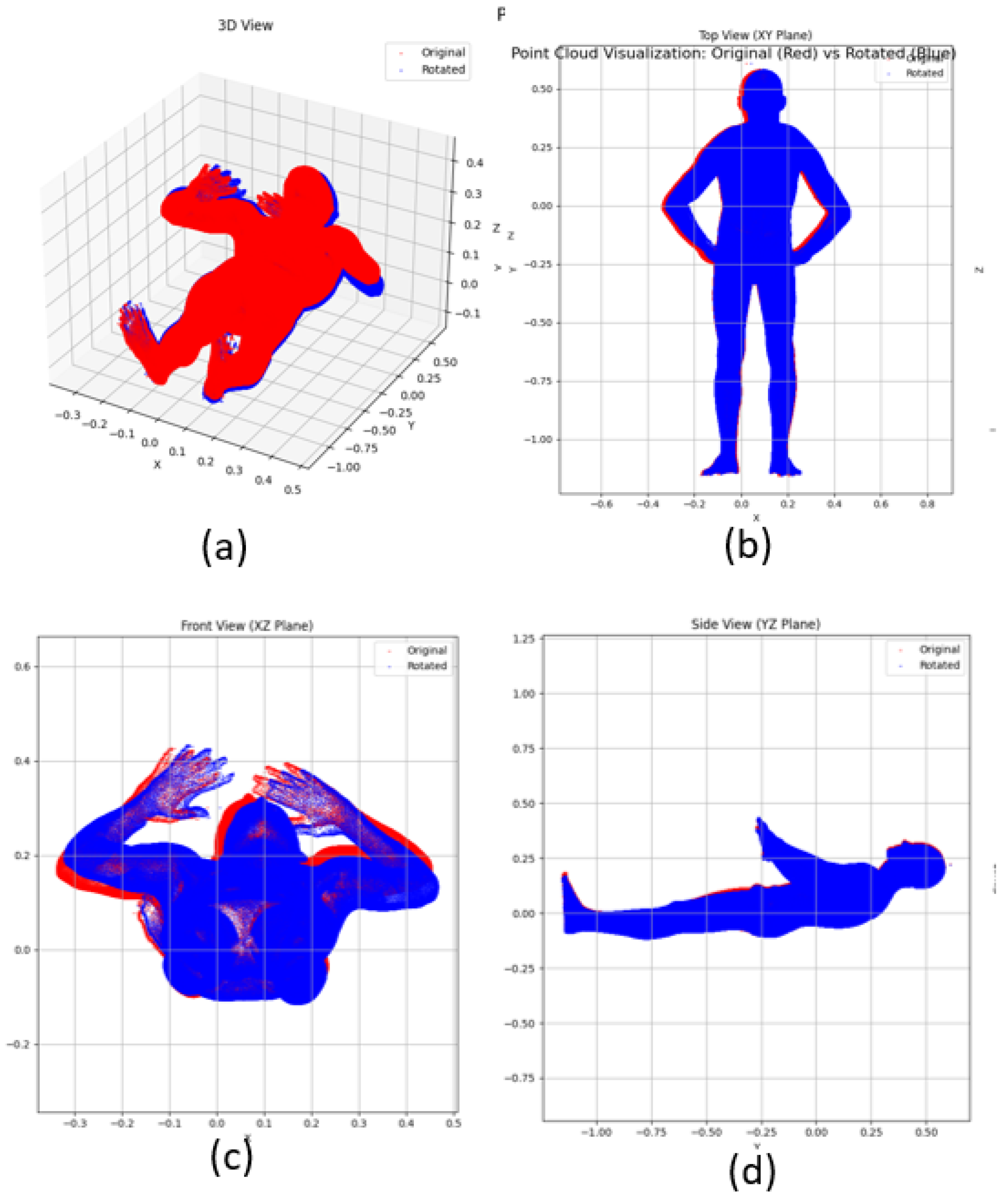

Table 1.
Comparison result of Basic Geometrical Shapes.
| Sphere (S) | Cone (C) | Cube (U) | |
|---|---|---|---|
| Sphere (S) | Ch = 0 | ||
| H = 0 | |||
| IGM = 0 | |||
| Cone (C) | Ch = 0.6188 | Ch = 0 | |
| H = 1.41 | H = 0 | ||
| IGM = 3.87 | IGM = 0 | ||
| Cube (U) | Ch = 0.8675 | Ch = 1.2016 | Ch = 0 |
| H = 0.9892 | H = 1.501 | H = 0 | |
| IGM = 1.6976 | IGM = 3.75 | IGM = 0 |
Table 2.
Comparison of Human Body Point Clouds.
| Man1 | Man2 | |
|---|---|---|
 |
 |
|
 |
IGM = 0 H = 0 Ch = 0 |
|
 |
IGM = 0.02988 H = 0.2661 Ch = 0.0888 |
IGM = 0 H = 0 Ch = 0 |
Table 3.
Comparison of Animal Point Clouds.
| Rabbit | Dragon | |
|---|---|---|
 |
IGM = 0 H = 0 Ch = 0 |
|
 |
IGM = 0.8552 H = 0.4598 Ch = 0.2779 |
IGM = 0 H = 0 Ch = 0 |
Table 4.
Comparison of Sculptural Point Clouds (Boy).
 |
 |
|
|---|---|---|
 |
IGM = 0 H = 0 Ch = 0 |
|
 |
IGM = 0.00878 H = 0.1342 Ch = 0.04429 |
IGM = 0 H = 0 Ch = 0 |
Disclaimer/Publisher’s Note: The statements, opinions and data contained in all publications are solely those of the individual author(s) and contributor(s) and not of MDPI and/or the editor(s). MDPI and/or the editor(s) disclaim responsibility for any injury to people or property resulting from any ideas, methods, instructions or products referred to in the content. |
© 2025 by the authors. Licensee MDPI, Basel, Switzerland. This article is an open access article distributed under the terms and conditions of the Creative Commons Attribution (CC BY) license (http://creativecommons.org/licenses/by/4.0/).
Copyright: This open access article is published under a Creative Commons CC BY 4.0 license, which permit the free download, distribution, and reuse, provided that the author and preprint are cited in any reuse.


