
Submitted:
31 December 2024
Posted:
03 January 2025
You are already at the latest version
Abstract
Water is the most important resource for life; however, the intensifying exploitation of water resources has led to significant degradation in water quality, particularly in rivers. This study investigates the potential of predictive models based on artificial intelligence techniques, such as Support Vector Machine (SVM) combined with mathematical approaches such as the Water Quality Index (WQI), to enhance the forecasting of water quality. We detail the methodology employed to construct these predictive models utilizing SVM, a specific WQI in conjunction with domain expertise. The models are developed from historical physicochemical parameter datasets from seven monitoring stations along a section of the Loa River in Antofagasta, Chile. The performance of the SVM model was rigorously validated using four key metrics: accuracy (acc), precision (p), recall (r), and F1-score. This paper elucidates the processes of dataset curation, and threshold optimization for influential physicochemical parameters. The approach presented herein is innovative, as it marks the first attempt to predict water quality specifically for the Loa River using SVM. The resultant models demonstrate robust performance metrics, achieving mean values of acc = 0.866, p = 0.849, r = 0.863, and F1-score = 0.847, positioning them competitively against analogous studies employing alternative methodologies in similar contexts.
Keywords:
Water quality prediction
; Surface water
; Support vector machine
; Machine learning
; Artificial Intelligence
1. Introduction
Water is the most important resource for life, therefore, the conservation of water quality (WQ) in surface water bodies has become a critical concern. However, the intensifying exploitation of water resources has led to significant degradation in WQ, particularly in rivers [1]. Although water covers 70% of the Earth's surface, the availability of water for aquatic life, agriculture, and human consumption is becoming increasingly scarce [2]. Thus, conserving the quality of freshwater is crucial for the preservation of the environment, human and animal consumption, and various industries, including agriculture.
Recent studies have focused on the variations in the total concentrations of elements, in surface water sources like rivers, especially in the context of mining activity, urbanization, and agricultural practices [3]. Studies such as those in [4,5], report that significant amounts of contaminants in water bodies, including rivers, can degrade WQ to levels unsuitable for human consumption. Moreover, specific characteristics of hydrographic basins and climatic variables (e.g., topography, soil composition, such as heavy metals, and climate data) can influence WQ in river systems [4].
These anthropogenic activities significantly impact river WQ, raising serious concerns about environmental sustainability and public health. Maintaining water quality at levels established by the World Health Organization (WHO) is particularly challenging in arid environments [5], where limited water availability, high evaporation rates, and industrial discharges exacerbate the problem [5,6,7].
According to [8,9], WQ can be assessed through parameters such as temperature, pH, electrical conductivity, and dissolved oxygen (DO). Additionally, other physicochemical parameters, including boron (B), copper (Cu), lead (Pb), and arsenic (As), must be considered due to their significant impact on WQ [9].
To calculate and classify WQ, mathematical approaches such as the Water Quality Index (WQI) are commonly used [1,10]. The WQI is widely regarded as an effective tool for expressing WQ because it provides a simple and consistent unit of measurement to describe the quality of water. However, the calculation of the WQI has traditionally relied on manual calculations and predefined formulas, which are prone to human errors, particularly in complex scenarios involving multiple interdependent parameters [10,11].
In recent years, alternative approaches, such as the use of Machine Learning (ML) techniques, have emerged as effective tools for calculating and monitoring WQ in surface water systems [9,12].
Studies [9,10,11,12,13,14,15,16] have shown the potential of integrating ML techniques with the WQI method to estimate discrete WQ values (labels) and classify these labels. These innovative approaches have been successfully applied in various regions; however, there is limited research implementing such methods in extremely arid environments like the Atacama Desert.
Northern Chile, particularly the Atacama Desert region, presents unique challenges for water resource management [17,18]. In this area, water is essential not only for human consumption and sanitation but also for critical industrial activities, including copper and lithium mining, agriculture, and livestock farming [4,17].
Although recent studies have applied ML techniques to analyze the influence of human activities on water quality parameters in river systems [19,20,21,22,23], these studies are often constrained by a limited number of watersheds and variables. Additionally, there is a lack of research specifically addressing the impact of heavy metal ion concentrations in rivers with topographies similar to the Loa River, a major water resource in the Atacama Desert region [9].
Given these gaps, integrating artificial intelligence and data science techniques offers an opportunity to analyze and predict WQ with greater accuracy, as demonstrated in previous research [23].
This study aims to complement previous work by using predictive variables to estimate and calculate WQ values based on national and international standards. Physicochemical parameters and WQ indicators were selected according to Chilean regulations [24,25] widely used by the Chilean government for water quality monitoring. Specifically, the study focuses on a section of the Loa River, addressing the critical need for accurate, data-driven methods to evaluate WQ in this highly vulnerable and industrialized arid region [26,27,28,29]. By leveraging ML techniques in combination with the WQI method, this research seeks to contribute to the understanding and management of WQ in the Atacama Desert, providing a framework that could be applied to similar environments worldwide.
In particular, this study introduces a novel approach using Support Vector Machine (SVM), a widely used ML technique, to develop WQ prediction models [27,28,29]. Unlike traditional methods as described in [23], this approach does not rely on the WQI but instead uses historical data on physicochemical parameters in a region characterized by high aridity, mineral concentration, and dependence on water resources to sustain the Atacama Desert ecosystem [9,30].
The remaining document is organized as follows: Section 2 introduces the study area and details the preparation and standardization of raw historical data obtained from the General Directorate of Water (DGA, for its acronym in Spanish) website. These data correspond to seven monitoring points for WQ physicochemical parameters. The Chilean regulations for WQ, threshold values used for labels generation and as input for the SVM modes are also described in Section 2. Section 3 presents the results, while Section 4 provides the conclusions of the study. Finally, the bibliography is included.
2. Materials and Methods
2.1. Study Area and Data Collection
The study area corresponds to the same section of the Loa River basin in the Antofagasta Region, Chile, as reported in previous work [9]. The Loa River spans over 400 km from its origin to its mouth in the Pacific Ocean. For this study, seven WQ monitoring stations around the city of Calama were selected (Figure 1). The selected area encompasses a segment of the Loa River before its confluence with its main tributary, the Salado River, and the segment after the river exits Calama. Additional details regarding the geographical location of the study area can be found in [9].
The monitoring stations are located at Finca, Escorial, Yalquincha, Salado River at Sifón Ayquina, before Salado River junction, Angostura, and Chiu Chiu well. The spatial location of the monitoring points is shown in Figure 1. Table 1 shows the sampling sites selected. From data analysis, the study area involves data processing to generate models. In this process, DGA historical data on the seven monitoring stations mentioned above are used.
Data on the physicochemical parameters of the seven monitoring stations described in Table 1 (1980–2023) were taken from the official DGA website (https://snia.mop.gob.cl/BNAConsultas/reportes). In this study historical data from 2020 to 2023 has been collected complement the dataset previously used in [9]. to create the dataset for training and testing, as described below. Most records available in the DGA historical database correspond to data collected during campaigns and published twice a year. In this way, the files with historical data from the DGA have at least two measurements for each year.
To facilitate the relationship with input data and the interpretation of monitoring geographical distribution, the following notation was used: L1 identifies the dataset corresponding to the monitoring point named “Salado River at Sifón Ayquina”. Similarly, L2, L3, L4, L5, L6, and L7 identify the remaining observation points shown in Table 1.
In our previous work described in [9], fifteen predictive variables were used for model training. Based on the results of that study, eight predictive variables were selected for training in the present research (see Table 2). This selection was guided by the importance of the variables, as determined using the Random Forest (RF) classification algorithm. The importance of each variable was calculated using the RF Information Gain Index metric, while also considering the Chilean regulations related to water quality (WQ) detailed in [24,25].
In this study, ensuring the robustness and reliability of real-time (on-site) monitoring datasets for physicochemical indicators was a critical focus, particularly due to their frequent susceptibility to scattered measurements and missing values. To address these data inconsistencies, the linear interpolation function (interp1) from Python's SciPy library was used. The interpolation process was configured with kind='cubic' to ensure smooth and continuous estimation of missing data points and fill_value="extrapolate" to handle extrapolations where necessary, thereby improving the dataset's reliability for subsequent analysis.
The threshold values for each physicochemical parameter (predictive variable), as specified in Table 2, were employed to calculate the Arithmetic Water Quality Index (AWQI) in accordance with the formula presented in Equation (1):
where the numerical factors that multiply each of the predictive variables were obtained in the previous study described in [9].
AWQI = pH*0.219+Mg*0.203+O2*0.183+Pb*0.133+
B*0.111+EC*0.059+As*0.048+Cu*0.039
B*0.111+EC*0.059+As*0.048+Cu*0.039
The AWQI was used to classify the water samples, generating three distinct labels for the depend variable WQ. The values of the labels and AWQI threshold values are detailed in Table 3.
2.2. Machine Learning-Based Model
As stated in the Introduction, the present study focuses on developing a model to predict water quality levels using historical data collected from seven sampling sites along a section of the Loa River. These predictions are achieved through the application of artificial intelligence (AI) techniques, specifically machine learning (ML) methods.
Prediction is a core topic in ML, involving the induction of a model from training data, which is then used to predict a target variable for new instances [31]. Various prediction algorithms are available, including logistic regression, neural networks, and decision trees, among others. These algorithms aim to build a model that learns to estimate the optimal value of a target variable based on training data, enabling reliable predictions for future instances within the same domain [32,33,34,35].
Currently, the literature contains a significant number of studies that use ML techniques to tasks such as analyze, predict or classify WQ in rivers. In particular, the literature contains papers such as [31,36] that highlight the use of SVM for perform the aforementioned tasks in water bodies such as rivers. ML techniques have been used also for calculate the WQI in a more general way respect to the traditional ways based on mathematical equations [37]. This combination can help to improve the performance of WQ approaches
Support vector machine (SVM) is a highly adaptable supervised ML that addresses complex regression, classification, and outlier detection problems by executing optimal data transformations [36]. These transformations create boundaries using an optimal hyperplane between the data points, based on pre-defined classes, labels or output. The hyperplane is positioned in such a way that it maximizes the margin between the classes. This margin signifies the widest gap that runs parallel to the hyperplane, without including any interna support vectors [38]. This gap is easy to define for linearly separable issues, but real-life scenarios can be more complex, therefore, the SVM algorithm attempt to maximize the margin between the support vectors, which can lead to incorrect classifications of smaller sections of the data points [36,39]. According to [12], the simulated outcome of an SVM model can be generated using Equation (2):
where is the predictive value, B is the bias term, is the coefficient of each input data point in the model, is the input data point, is the kernel functionused to compute the similarity between the input data point and the new data point .
The parameter is used to control penalization when training instances are classified incorrectly. For a high value of . SVM tends to generate a smaller margin at the risk of overfit. A small value of results in more erroneous classifications at the expense of training precision [37].
2.3. Methodology
The methodology applied in this study include the following steps.
- Data preparation. The physicochemical data corresponding to the monitoring station described in Table 1 were accessed from the official DGA website. Data corresponding to variables indicated in Table 2 were prepared and standardized using spline as explained before in order to use on the training, and testing the models.
- Model generation. This step consists of training for each sampling site using SVM algorithm. For each dataset, part of the data is used for training, while the rest is used for validation at a 70-30 ratio.
- Model visualization and quality analysis. In this stage, models’ results were visualized and analyzed in order to determine their validity. Evaluation consisted of check the performance of each model generated with SVM for each dataset. To do this and in a similar way to [35], values of certainty such as accuracy (Acc), recall (r), precision (p) and F1 Score were used. The way these values of certainty were calculated and their importance for model quality are described below. This state also includes a result analysis, this analysis aimed at establishing if the results obtained are useful for the WQ classification for each sample site.
To make the model quality analysis in stage 3 above, a confusion matrix was considered. Following previous studies such as [9,35], confusion matrix values can be used to calculate Acc, p, r and F-1 s. The way these indicators is described in Equations (3) – (6).
where a, b, c and d represent the true positive case, false positives case, true negatives case, and false positives case, respectively. The Acc corresponds to the ratio of correctly classified samples to the total number of samples in the dataset; p represents the proportion of true positive cases among all elements predicted as positive, while r denotes the proportion of true positive cases among all actual positive elements. The F1 score, in turn, can be interpreted as the harmonic mean of p and r.
Acc = (a+b)/(a+b+c+d
p = a/(b+c)
r = (a+d)/(b+c)
F1 score = 2*(p*r)/(p+r)
3. Results
The result of water quality classification for each sampling site described in Table 1 is covered in this section. SVM training was conducted independently with L1, L2, L3, L4, L5, L6, and L7 datasets, using the same algorithm parameter settings. For training a total of 308 records have been used.
At the present study, the SVM classifier with the linear kernel for the classification task was used, this includes the test_size = 0.3, random_state = 42 for the split data. To do the training, labels 0, 1, and 2, for low, middle, and high values corresponding to WQ classes described in Table 3 were used.
Table 4 illustrates the confusion matrices for each training session. In Table 4 the results show that classification precision is always over 92% for the three ranges. This can be interpreted as a good approximation of the SVM-generated models to what is actually observed in each dataset.
Table 5 summarizes these metric values across all datasets. In summary, Acc from SVM training was 86.6%, a relatively high value of correctly classified samples, compared to the standard value for this type of training. The average value of F1-score was 0.866, which can be interpreted as a model precision closed to 87%.
Likewise, the precision (p) average of the three labels was 0.849, which may be interpreted as a low dispersion of data correctly classified from input data. In addition, the recall (r) average was 0.863, which may be interpreted as a relatively high proportion of true positive cases among all actual positive elements.
As Therefore, the SVM method generates good models that can be used for new cases, given the level of certainty of the model quality and the verification of outliers described above.
A limitation of this study is that the model was trained with data from only seven water quality monitoring stations in the Loa River basin, despite DGA monitoring more than 30 points in this basin.
Based on the training results, it can be deduced that the water quality in the study area is poor. This finding is consistent with previous works, such as [6,9,28].
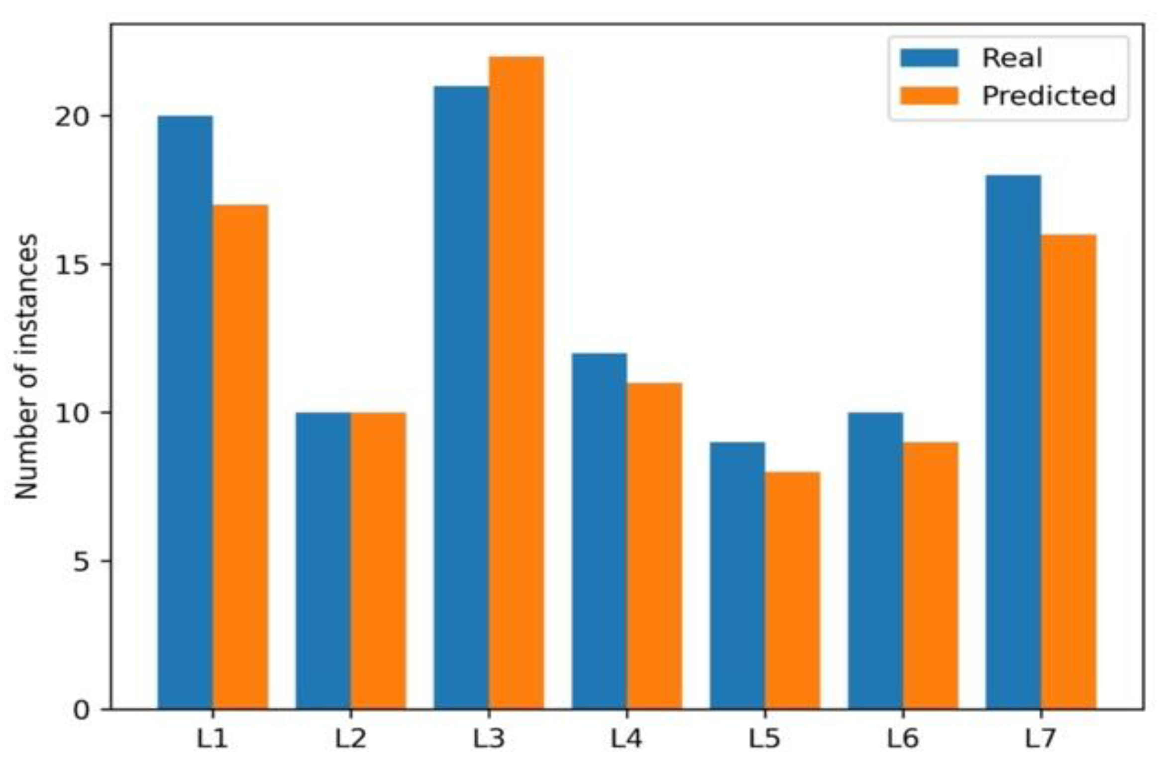
Figure 1 shows the real vs. the predicted values using SVM, according to the classification labels. As figure 1 detailed, the predictions closely align with real values.
Figure 2.
Comparative graph of actual vs predicted values using SVM.
4. Conclusions
This study proposes a framework based on Support vector machine (SVM) and physicochemical parameter analysis to predict Water quality (WQ) at seven sampling sites along the Loa River, Chile. This study uses datasets prepared following the data preparation process described in [9], but these datasets were updated with real and recent data. The methodology uses these datasets and the SVM's robustness to optimize prediction accuracy.
The approach integrates historical data on physicochemical parameters, Chilean WQ regulations, and expert knowledge, specifically tailored to a region characterized by high aridity, mineral concentration, and water resources essential for sustaining the Atacama Desert ecosystem. Unlike traditional methods, this study develops a WQ prediction model without relying on the Water Quality Index.
Model performance was evaluated using metrics such as accuracy (0.866), precision (0.849), recall (0.863), and F1-score (0.847), demonstrating reliable predictive capabilities. The results suggest the potential to adapt this methodology for deriving threshold values specific to the Loa River and expanding its application to other hydrometric stations in the basin.
Future research could extend this framework to other river basins with varying geochemical conditions, enabling the development of generalized predictive models for diverse environmental contexts.
Author Contributions
Conceptualization, Victor Flores, Adel Elmaghraby; methodology, Victor Flores; software, Victor Flores; validation, Victor Flores, Adel Elmaghraby, Rafael Martinez; formal analysis, Rafael Martinez, Victor Flores; writing— Victor Flores, Adel Elmaghraby. All authors have read and agreed to the published version of the manuscript.
Funding
This research received no external funding.
Data Availability Statement
The raw data used in this study are openly available in .
Conflicts of Interest
The authors declare no conflicts of interest.
References
- Nayak, B.; Panda, P. K. A Comprehensive Review of Water Quality Analysis. International Journal of Image and Graphics 2024, 1–15. [Google Scholar] [CrossRef]
- Adangampurath, S.; Pulikkal, A. Effects of seasonal variation on the water quality of the Kadalundi river, India: evaluation of water quality indices, physicochemical and biological parameters. International Journal of River Basin Management 2024, 1–12. [Google Scholar] [CrossRef]
- Wang Z.; Wei J.; Peng W.; Zhang R. and H. Zhang. Contents and spatial distribution patterns of heavy metals in the hinterland of the Tengger Desert. China. J. Arid. Land 2022, 14, 1086–1098. [Google Scholar] [CrossRef]
- López-Berenguer G.; Pérez-García J; García-Fernández A.; Martínez-López E. High levels of heavy metals detected in feathers of an avian scavenger warn of a high pollution risk in the Atacama Desert (Chile). Arch. Environ. Contam. Toxicol 2021, 81, 227–235. [Google Scholar] [CrossRef]
- Kereszturi, A. Unique and potentially Mars-relevant flow regime and water sources at a high Andes-Atacama site. Astrobiology 2020, 20, 723–740. [Google Scholar] [CrossRef]
- Pino-Vargas, E.; Chavarri-Velarde, E. Evidence of climate change in the hyper-arid region of the southern coast of Peru, head of the Atacama Desert. Tecnol. Cienc. del Agua 2022, 13, 333–375. [Google Scholar] [CrossRef]
- Chen M.; Tan Y.; Xu X,; Lin Y. Identifying ecological degradation and restoration zone based on ecosystem quality: A case study of Yangtze River Delta. Applied Geography 2024, 16. [Google Scholar] [CrossRef]
- Huang, H.; Lu, J. Identification of river water pollution characteristics based on projection pursuit and factor analysis. Environ. Earth Sci 2014, 72, 3409–3417. [Google Scholar] [CrossRef]
- Flores, V.; Bravo, I.; Saavedra, M. Water Quality Classification and Machine Learning Model for Predicting Water Quality Status—A Study on Loa River Located in an Extremely Arid Environment: Atacama Desert. Water 2023, 15, 1–18. [Google Scholar] [CrossRef]
- Chidiac S.; El Najjar P.; Ouaini O; El Rayess Y.; El Azzi D. A comprehensive review of water quality indices (WQIs): history, models, attempts and perspectives. Reviews in Environmental Science and Bio/Technology 2023, 22, 349–395. [Google Scholar] [CrossRef]
- Huang, Z.; Sun, R.; Wang, H.; Wu, X. Trends and Innovations in Surface Water Monitoring via Satellite Altimetry: A 34-Year Bibliometric Review. Remote Sensing 2024, 16, 1–22. [Google Scholar] [CrossRef]
- Abbas, F.; Cai, Z.; Shoaib, M.; Iqbal, J.; Ismail, M.; Alrefaei A., F.; Albeshr M., F. Machine learning models for water quality prediction: a comprehensive analysis and uncertainty assessment in Mirpurkhas, Sindh, Pakistan. Water 2024, 16, 1–19. [Google Scholar] [CrossRef]
- Frincu R., M. Artificial intelligence in water quality monitoring: a review of water quality assessment applications. Water Quality Research Journal 2024, 59, 1–13. [Google Scholar] [CrossRef]
- Chen, X.; Wang, Y.; Jiang, L.; Huang, X.; Huang, D.; Dai, W.; Wang, D. Water quality status response to multiple anthropogenic activities in urban river. Environmental Science and Pollution Research 2023, 30, 3440–3452. [Google Scholar] [CrossRef]
- Bui M., T.; Yáñez-Godoy, H.; Elachachi S., M. Assessment of the Implications and Challenges of Using Artificial Intelligence for Urban Water Networks in the Context of Climate Change When Building Future Resilient and Smart Infrastructures. Journal of Pipeline Systems Engineering and Practice 2024, 16, 03124004. [Google Scholar] [CrossRef]
- Chhipi-Shrestha, G.; Mian H., R.; Mohammadiun, S.; Rodriguez, M.; Hewage, K.; Sadiq, R. Digital water: artificial intelligence and soft computing applications for drinking water quality assessment. Clean Technologies and Environmental Policy 2023, 25, 1409–1438. [Google Scholar] [CrossRef]
- M. Méndez, M. Prieto and M. Godoy. Production of subterranean resources in the Atacama Desert: 19th and early 20th-century mining/water extraction in The Taltal district, northern Chile. Political Geogr. 2020, 81, 1–15. [Google Scholar] [CrossRef]
- K. Lizama-Allende C.; Rómila E.; Leiva P.; Guerra; J. Ayala. Evaluation of surface water quality in basins of the Chilean Altiplano-Puna and implications for water treatment and monitoring. Environmental Monitoring and Assessment 2022, 194, 1–28. [Google Scholar] [CrossRef]
- Park, J.; Seong, B.; Park, Y.; Lee W., H.; Heo, T. Y. Explainable artificial intelligence for the interpretation of ensemble learning performance in algal bloom estimation. Water Environment Research 2024, 96, e11140. [Google Scholar] [CrossRef]
- Tian, P.; Xu, Z.; Fan, W.; Lai, H.; Liu, Y.; Yang, P.; Yang, Z. Exploring the effects of climate change and urban policies on lake water quality using remote sensing and explainable artificial intelligence. Journal of Cleaner Production 2024, 475, 1–10. [Google Scholar] [CrossRef]
- Dinar, H.; Al-Qaisi A., Z.; Jasim H., K. Optimization Model for Climatic Change Impact on the Water Quality of Al-Hilla River, Iraq. Applied Chemical Engineering 2024, 7. [Google Scholar] [CrossRef]
- Das, A.; Chowdhury A., R. Empowering sustainable water management: the confluence of artificial intelligence and Internet of Things. In Current Directions in Water Scarcity Research 2024, 8, 275–291. [Google Scholar]
- Masud M., M.; Shamem A. S., M.; Saif A. N., M.; Bari M., F.; Mostafa, R. The role of artificial intelligence in sustainable water management in Asia: a systematic literature review with bibliographic network visualization. International Journal of Energy and Water Resources 2024, 1–19. [Google Scholar] [CrossRef]
- INN-NCh1333. Official Chilean Standard NCh1333 Water Quality Requirements for Different Uses. INN, National Institute for Standardization 1987, Santiago, Chile.
- INN-NCh409. Official Chilean Drinking Water Standard. INN, National Institute of Standardization 2005, Santiago, Chile.
- Narvaez-Montoya, C.; Mahlknecht, J.; Torres-Martínez J., A.; Mora, A.; Pino-Vargas, E. FlowSOM clustering–A novel pattern recognition approach for water research: Application to a hyper-arid coastal aquifer system. Science of The Total Environment 2024, 915, 1–12. [Google Scholar] [CrossRef]
- Jayakumar, D.; Bouhoula, A.; Al-Zubari W., K. Unlocking the Potential of Artificial Intelligence for Sustainable Water Management Focusing Operational Applications. Water 2024, 16, 1–17. [Google Scholar] [CrossRef]
- Pino-Vargas, E.; Espinoza-Molina, J.; Chávarri-Velarde, E.; Quille-Mamani, J.; Ingol-Blanco, E. Impacts of Groundwater Management Policies in the Caplina Aquifer, Atacama Desert. Water 2023, 15, 2610. [Google Scholar] [CrossRef]
- Díaz F., P.; Latorre, C.; Carrasco-Puga, G.; Wood J., R.; Wilmshurst J., M.; Soto D., C.; Gutiérrez, R. A. Multiscale climate change impacts on plant diversity in the Atacama Desert. Global Change Biology 2019, ƒ25, 1733–1745. [Google Scholar] [CrossRef]
- Bonnail, E.; Cruces, E.; Rothäusler, E.; Oses, R.; García, A.; Ulloa, C.; Abad, M. An Integrated Approach for the Environmental Characterization of a Coastal Area in the Southern Atacama Desert. Applied Sciences 2023, 13, 6360. [Google Scholar] [CrossRef]
- Yao, Y.; Chen, Y.; Li, X.; Zhang, B.; Zhu, Z.; Gao, X.; Hu, Y. Water Quality Prediction of Small-Micro Water Body Based on the Intelligent-Algorithm-Optimized Support Vector Machine Regression Method and Unmanned Aerial Vehicles Multispectral Data. Sustainability 2024, 16, 1–15. [Google Scholar] [CrossRef]
- V. Flores. Determination of Trees Predictive Models for Surface Roughness in High-Speed Machining (HSP): A Study in Steel and Aluminum Metalworking Industry, in: M. Ferreira (Ed), Research Highlights in Mathematics and Computer Science, volume 4, BP International, India 2023, 42-66. [CrossRef]
- Dritsas, E.; Trigka, M. Efficient Data-Driven Machine Learning Models for Water Quality Prediction. Computation 2023, 11, 16–23. [Google Scholar] [CrossRef]
- Haghiabi, A.; Nasrolahi, A.; Parsaie, A. Water quality prediction using machine learning methods. Water Quality Research Journal 2018, 53, 3–13. [Google Scholar] [CrossRef]
- Flores, V.; Henriquez, N.; Ortiz, E.; Martinez, R.; Leiva, C. Random Forest for generating recommendations for predicting copper recovery by flotation. IEEE Latin America Transactions 2024, 22, 443–450. [Google Scholar] [CrossRef]
- Du S., X.; Wu X., L.; Wu T., J. Support vector machine for ultraviolet spectroscopic water quality analyzers. Chinese Journal of Analytical Chemistry 2004, 32, 1227–1230. [Google Scholar]
- Masood, A.; Niazkar, M.; Zakwan, M.; Piraei, R. A machine learning-based framework for water quality index estimation in the Southern Bug River. Water 2023, 15, 1–14. [Google Scholar] [CrossRef]
- Krishnan, S.; Manikandan, R. Water quality prediction: a data-driven approach exploiting advanced machine learning algorithms with data augmentation. Journal of Water and Climate Change 2024, 15, 431–452. [Google Scholar] [CrossRef]
- Gai, R.; Guo, Z. A water quality assessment method based on an improved grey relational analysis and particle swarm optimization multi-classification support vector machine. Frontiers in Plant Science 2023, 14, 1099668. [Google Scholar] [CrossRef]
Figure 1.
Study area.
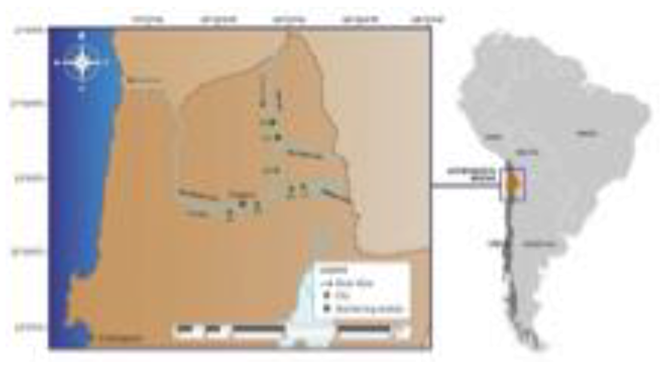

Table 1.
sampling sites in the Loa River basin.
| Sampling site | Location name | S latitude | W longitude |
|---|---|---|---|
| L1 | Salado River at Sifón Ayquina | 22°17′21″ | 68°20′41″ |
| L2 | Chiu Chiu Well | 22°20′22″ | 68°35′56″ |
| L3 | Loa River before Salado River Intersection | 22°21′51″ | 68°39′06″ |
| L4 | Loa River at Escorial | 22°26′43″ | 68°53′25″ |
| L5 | Loa River at Yalquincha | 22°27′02″ | 68°52′45″ |
| L6 | Loa River at Angostura | 22°27′00″ | 68°43′00″ |
| L7 | Loa River at Finca | 22°30′34″ | 68°59′27″ |
Table 2.
Physicochemical parameters, their ranges, and relative weights, all obtained from the previous work described in [9].
Table 2.
Physicochemical parameters, their ranges, and relative weights, all obtained from the previous work described in [9].
| Physicochemical parameter | Maximum value [24] |
Maximum value [25] |
Relative weight [9] |
|---|---|---|---|
| pH | (6.5, 9.5) | (6.5, 8.5) | 0,219 |
| Magnesium (Mg) | ≤135 mg/L | ≤125 mg/L | 0,203 |
| Dissolved Oxygen (O2) | ≤20 mgO2/L | ≤20 mgO2/L | 0,183 |
| Lead (Pb) | ≤0.5 mg/L | ≤0.05 mg/L | 0,140 |
| Boron (B) | ≤0.05 mg/L | ≤0.05 mg/L | 0,111 |
| Electric Conductivity (EC) | ≤3000µ mhos/cm | ≤3000µ mhos/cm | 0,059 |
| Arsenic (As) | ≤0.3 mg/L | ≤0.3 mg/L | 0,048 |
| Copper (Cu) | ≤3.0 mg/L | ≤2.0 mg/L | 0,039 |
Table 3.
AWQI threshold values and discrete values (labels) for Water Quality (WQ).
| AWQI ranges | WQ value |
|---|---|
| AWQI <25 | high |
| 25 ≤ AWQI < 60 | medium |
| AWQI ≥ 60 | low |
Table 4.
Predictive variables ranges and class labels. Graphs (a), (b), (c), (d), (e), (f), and (g) correspond to the L1, L2, L3, L4, L5, L6, and L7 monitoring stations, respectively.
Table 4.
Predictive variables ranges and class labels. Graphs (a), (b), (c), (d), (e), (f), and (g) correspond to the L1, L2, L3, L4, L5, L6, and L7 monitoring stations, respectively.
| True low | True medium | true high | ||
|---|---|---|---|---|
| (a) | Pred. low | 17 | 0 | 0 |
| Pred medium | 0 | 3 | 0 | |
| Pred high | 0 | 2 | 0 | |
| (b) | Pred. low | 2 | 0 | 1 |
| Pred medium | 0 | 10 | 2 | |
| Pred high | 0 | 0 | 0 | |
| (c) | Pred. low | 21 | 0 | 0 |
| Pred medium | 0 | 1 | 1 | |
| Pred high | 0 | 0 | 0 | |
| (d) | Pred. low | 10 | 0 | 0 |
| Pred medium | 1 | 0 | 0 | |
| Pred high | 0 | 3 | 0 | |
| (e) | Pred. low | 7 | 2 | 0 |
| Pred medium | 1 | 0 | 0 | |
| Pred high | 0 | 3 | 0 | |
| (f) | Pred. low | 10 | 0 | 0 |
| Pred medium | 0 | 0 | 0 | |
| Pred high | 0 | 0 | 0 | |
| (g) | Pred. low | 2 | 3 | 0 |
| Pred medium | 0 | 11 | 2 | |
| Pred high | 0 | 2 | 0 |
Table 5.
Performance Metrics for WQ predictive models: Accuracy (Acc), Recall(r), Precision (p), and F1-Score(F1).
Table 5.
Performance Metrics for WQ predictive models: Accuracy (Acc), Recall(r), Precision (p), and F1-Score(F1).
| Sampling site | Acc | r | p | F1 |
|---|---|---|---|---|
| L1 | 0.850 | 0.850 | 0.722 | 0,781 |
| L2 | 0.923 | 0.923 | 1.000 | 0.953 |
| L3 | 0.954 | 0.954 | 0.911 | 0.932 |
| L4 | 0.909 | 0.909 | 0.826 | 0.865 |
| L5 | 0.700 | 0.700 | 0.787 | 0.741 |
| L6 | 1.000 | 1.000 | 1.000 | 1.000 |
| L7 | 0.722 | 0.721 | 0.697 | 0.656 |
Disclaimer/Publisher’s Note: The statements, opinions and data contained in all publications are solely those of the individual author(s) and contributor(s) and not of MDPI and/or the editor(s). MDPI and/or the editor(s) disclaim responsibility for any injury to people or property resulting from any ideas, methods, instructions or products referred to in the content. |
© 2025 by the authors. Licensee MDPI, Basel, Switzerland. This article is an open access article distributed under the terms and conditions of the Creative Commons Attribution (CC BY) license (http://creativecommons.org/licenses/by/4.0/).
Copyright: This open access article is published under a Creative Commons CC BY 4.0 license, which permit the free download, distribution, and reuse, provided that the author and preprint are cited in any reuse.


