
Submitted:
31 December 2024
Posted:
31 December 2024
You are already at the latest version
Abstract
The numerical simulation of control of spring-mass-damper (SMD) systems offer critical insights into dynamical systems and computational methodologies. This study provides a comprehensive comparative analysis of implementing SMD systems across two prominent open-source scientific computing platforms: Python and R. By examining both open-loop and closed-loop system configurations, the research investigates the computational performance, numerical accuracy, and implementation characteristics of these platforms. Utilizing an idealized one-dimensional SMD system with a Proportional-Integral-Derivative (PID) controller, the study conducted extensive numerical simulations and statistical performance analyses. Results revealed Python's significant advantages in execution speed, achieving up to 63.57% reduction in runtime for controlled system simulations, while R demonstrated superior consistency in execution and memory usage. The controlled system demonstrated exceptional performance, with a final position error of merely 0.4% and enhanced damping characteristics. This work not only bridges theoretical stability analysis with empirical performance insights but also promotes reproducibility and transparency in computational dynamics research by leveraging open-source platforms.
Keywords:
Control systems
; Cross-platform implementation
; Numerical methods
; Performance analysis
; Spring-mass-damper dynamics
1. Introduction
The numerical analysis and computational implementation of spring-mass-damper (SMD) systems present rich opportunities for investigating fundamental questions in dynamical systems and numerical methods. These systems, while conceptually straightforward, embody essential characteristics of more complex dynamical systems and serve as valuable benchmarks for evaluating numerical methods and computational frameworks. With the rise of open science practices and increasing demands for research transparency [1], the choice of computational platforms becomes particularly significant in ensuring both mathematical rigor and reproducibility.
The mathematical structure of SMD systems manifests across multiple scales of computational physics and engineering analysis, from simple mechanical oscillators to sophisticated control systems. Our investigation encompasses both open-loop and closed-loop configurations, allowing us to examine how different numerical methods handle varying degrees of system complexity. In the current landscape, where open science platforms are reshaping scientific communication [2], implementing these systems in accessible, transparent environments becomes crucial for validating both theoretical predictions and numerical approximations. Two leading open-source platforms, Python and R, have emerged as dominant choices for scientific computing, each offering distinct approaches to numerical computation and algorithm implementation.
Contemporary scientific computing increasingly relies on these open-source platforms, which align with broader movements toward research transparency and reproducibility. Python’s scientific computing ecosystem, built around NumPy and SciPy, exemplifies how open-source tools can enable sophisticated numerical computations while maintaining accessibility. The platform’s implementation of variable-step, variable-order methods provides particular insight into handling stiff differential equations and adaptive error control. Similarly, R’s statistical computing framework, particularly through packages like deSolve, demonstrates how community-driven development can produce robust tools for complex mathematical modeling, offering unique perspectives on numerical stability and error propagation. The computational challenges become particularly evident when implementing variable-step, variable-order methods for these systems, especially in the context of PID control where system stiffness can vary significantly. As scientific practices evolve toward greater openness and accessibility [3], the ability to examine and validate implementation details becomes crucial. Both Python and R provide transparent implementations of numerical methods, allowing researchers to understand and verify the underlying algorithms - a key advantage for studying numerical stability, convergence properties, and error accumulation in long-time integration.
The significance of this comparative study extends beyond mere platform evaluation, addressing fundamental questions in computational mathematics and numerical analysis. In an era where research integrity increasingly depends on computational reproducibility [2], understanding the relative strengths and limitations of different open-source implementations becomes crucial. First, the choice between Python and R affects not only computational performance but also numerical accuracy and stability, particularly in handling stiff systems and adaptive step size control. Second, as open-source platforms continue to evolve, systematic comparisons help inform both theoretical understanding of numerical methods and their practical implementation. Third, with the growing emphasis on research transparency, these platforms provide an ideal foundation for studying how different numerical schemes behave in both open and closed-loop dynamical systems, contributing to both applied mathematics and computational science.
2. Methods
2.1. Mathematical Formulation
Our analysis began with an idealized one-dimensional SMD system, consisting of a point mass kg coupled to both an ideal linear spring of stiffness N/m and a viscous damper with coefficient Ns/m, as illustrated in Figure 1. The system’s idealization encompassed several key simplifications: the mass behaved as a point particle devoid of rotational dynamics, the spring exhibited perfectly linear behavior following Hooke’s law with negligible mass, the damper provided purely viscous damping, and the system operated in the absence of friction or additional constraints. All connections between components were considered rigid and massless, ensuring that the system’s behavior was governed solely by the interplay of inertial, elastic, and dissipative forces.
The mathematical model emerged directly from Newton’s Second Law, which stated that the sum of forces acting on the mass equaled the product of mass and acceleration. In our system, three distinct forces acted on the mass: the spring force following Hooke’s law (), the damping force proportional to velocity (), and an external force . The negative signs in the spring and damping forces indicated their opposition to displacement and motion, respectively. Applying Newton’s Second Law and substituting these forces yielded the fundamental equation of motion:
which, upon substituting our system parameters, became:
To facilitate modern control analysis and implementation, we transformed this second-order differential equation into state-space form. The transformation introduced a state vector , where represented position and represented velocity. This choice of states provided clear physical insight: captured the system’s configuration while described its instantaneous motion. The resulting state equations took the form:
which could be expressed in the canonical matrix form:
For precise position control, we implemented a Proportional-Integral-Derivative (PID) controller with carefully tuned gains: N/m for proportional action, N/(ms) for integral action, and N·s/m for derivative action. Given a desired position trajectory , the control law synthesized the input force as:
The integral action in the controller necessitated augmenting our state space with an additional state variable representing the accumulated position error. This augmentation led to the complete closed-loop dynamics:
The complete system architecture, including both open-loop and closed-loop configurations, was illustrated in Figure 2. This representation explicitly showed the signal flow and system interconnections, highlighting the fundamental difference between direct force input and feedback control strategies.
2.2. Numerical Implementation
The numerical solution of our SMD system required careful consideration of both accuracy and stability, particularly given the potential stiffness introduced by the control parameters. Our implementation leveraged the Python scientific computing ecosystem, specifically employing NumPy [4] for array operations and the Livermore Solver for Ordinary Differential Equations with Automatic method switching (LSODA) through SciPy’s integrate module [5]. For data manipulation and storage of results, we utilized the pandas library [6], which provided efficient DataFrame structures for handling time series data and simulation outputs.
The core of our numerical approach lay in the transformation of our continuous-time system into a form suitable for computational solution. For the open-loop system, we began with the state-space representation derived in our mathematical formulation. The solver required a system model function that returned the state derivatives:
where represented our state vector, and F was the input force. This formulation expanded to our specific parameter values:
The LSODA algorithm employed an adaptive strategy, automatically switching between methods optimal for stiff and non-stiff regions of the solution. For non-stiff regions, it utilized Adams-Moulton methods of orders 1-12, which took the general form:
where h represented the step size and were the method coefficients. For stiff regions, the solver switched to backward differentiation formulas (BDF):
where and were the BDF coefficients.
The simulation time domain was discretized with careful attention to numerical stability and accuracy requirements. We employed a base step size of seconds over a simulation interval seconds for the open-loop system and seconds for the controlled system. This discretization resulted in:
where represented the total number of time steps.
The input force profile was generated through a carefully designed transition function to avoid numerical artifacts. For a step input from to occurring between times and , we implemented a linear transition:
with specific values N, N, s, and s for the open-loop case.
For the closed-loop system, the numerical implementation became more intricate due to the PID control law. The augmented state vector required modification of our system model to incorporate the integral term:
The numerical solver handled this augmented system with the same adaptive strategy, but special care was taken in the initialization and update of the integral term to prevent numerical drift. The desired position trajectory followed a similar smooth transition profile, but with values scaled to position units: m to m between s and s.
Error control in our numerical solution was maintained through careful monitoring of local truncation error at each step:
where represented a higher-order approximation used for error estimation. The step size was adaptively adjusted based on this error estimate:
with p denoting the current method order and as our specified tolerance.
The complete implementation was organized into modular Python classes, following object-oriented programming principles, which facilitated easy modification and extension of the system model and control algorithms. All numerical computations were performed using Python, with NumPy, SciPy, and pandas. For comparative validation and robustness testing, parallel implementations were developed in R using the deSolve package [7] for differential equation solving and the tidyverse ecosystem [8] for data manipulation and visualization. The results from both implementations showed excellent agreement, providing confidence in the numerical accuracy of our solutions.
2.3. Stability Analysis
Our stability analysis methodology incorporated multiple theoretical frameworks to thoroughly assess both open-loop and closed-loop system behavior. Following [9], we employed three complementary approaches of eigenvalue analysis, Routh-Hurwitz criterion, and Bounded-Input, Bounded-Output (BIBO) stability assessment, with each method providing unique insights into the system’s dynamic characteristics.
The first stage of our analysis centered on eigenvalue decomposition. For a linear time-invariant system, stability required that all eigenvalues had negative real parts [10]. The analysis began with our open-loop system matrix:
from which we formulated the characteristic equation through determinant evaluation:
Following [11], we determined two fundamental parameters characterizing the system’s behavior. The natural frequency represented the system’s undamped oscillation rate, while the damping ratio characterized the decay rate of oscillations:
The nature of system damping played a crucial role in determining the transient response characteristics. As derived by [9], the damping ratio indicated an underdamped system, as it fell within the range . In such cases, the system’s free response exhibited oscillatory behavior with exponential decay. The complete solution took the form:
where represented the damped natural frequency, and A and were determined by initial conditions. This underdamped characteristic arose from our physical parameters, with the mass-spring-damper combination producing complex conjugate eigenvalues .
Asymptotic stability analysis followed the theoretical framework of [10], which required examination of the system’s long-term behavior as . For our linear system, asymptotic stability demanded that all eigenvalues had strictly negative real parts. The real component of our eigenvalues, , being negative, ensured exponential decay of any initial conditions or disturbances. This stability manifested through the exponential term in the system response, which approached zero as time increased.
The Routh-Hurwitz stability criterion [12] provided an algebraic method for determining stability without explicit eigenvalue calculation. For our second-order characteristic equation:
we constructed the Routh array and examined its first column entries:
The stability conditions derived from the Routh array required all elements in its first column to be positive. Following [13], this translated to the requirements , , and , which were all satisfied in our system, confirming stability from an algebraic perspective.
The BIBO stability assessment followed [14] methodology, focusing on the system’s transfer function:
This approach required examination of both the positivity of denominator coefficients and the Hurwitz stability of the denominator polynomial. Our transfer function satisfied both conditions, as all denominator coefficients were positive and matched the previously analyzed characteristic equation.
For the closed-loop analysis with PID control, we extended these methodologies to the augmented third-order system. The characteristic equation expanded to include controller parameters:
necessitating an expanded Routh array for stability analysis:
The relationship between damping and asymptotic stability was further illuminated through the root locus analysis detailed by [13]. The characteristic equation roots, or system poles, lying in the left half of the complex plane (Re) guaranteed that any oscillations would eventually decay. The distance of these poles from the imaginary axis, determined by , dictated the decay rate, while their imaginary components determined the oscillation frequency.
The robustness of our closed-loop system was examined through the method of [15], which analyzed the loop transfer function:
This transfer function formed the basis for determining critical frequency-domain stability margins, providing insight into the system’s robustness against parameter variations and modeling uncertainties. The stability margins derived from this transfer function offered quantitative measures of how much gain variation and phase shift the system could tolerate while maintaining stability.
2.4. Statistical Framework for Performance Analysis
Building upon the system dynamics simulation framework described before, we developed and implemented a comprehensive statistical analysis approach to compare the performance characteristics of Python and R implementations. All experiments were conducted on a ThinkPad P52s laptop running Fedora Linux 39 (Budgie) x86_64, equipped with an Intel i7-8550U processor (8 threads, 4.000GHz). Given that our numerical simulations primarily involved CPU-bound computations without parallel processing requirements, this standard laptop configuration provided an adequate testing environment representative of typical scientific computing setups in practice.
Our analysis pipeline utilized Python’s scientific computing stack, including NumPy for numerical computations [4], SciPy for statistical testing [5], pandas for data management [6], and Seaborn for statistical visualization [16]. Following established practices in performance evaluation [17] and statistical sampling theory [18], we collected measurements for each implementation type and language after discarding warm-up runs. These warm-up runs were essential to mitigate the effects of just-in-time compilation and cache warming, as demonstrated by Herho et al. [19], Herho et al. [20], Herho et al. [21].
Our analysis began with fundamental statistical measures for each implementation-language pair . Following the recommendations of Jain [22] for computer systems performance analysis, we computed the central tendency and dispersion metrics:
where represents the mean performance measure, n is the number of observations, and is the k-th performance measurement for implementation i and language j.
where denotes the standard deviation of the performance measurements.
where represents the coefficient of variation.
The coefficient of variation in Equation (28) proved particularly valuable for performance comparisons, as it provided a dimensionless measure of variability [23]. Following [24] and recent performance analysis guidelines [25], we interpreted values below 5% as very consistent performance, 5–10% as good consistency, 10–15% as moderate variability, and above 15% as high variability.
Distribution shape analysis was crucial for understanding performance characteristics and selecting appropriate statistical tests [26]. We computed skewness () and kurtosis ():
where represents the skewness of the distribution.
where represents the excess kurtosis of the distribution.
These shape parameters were essential for detecting potential performance anomalies and understanding the underlying performance distribution patterns [27].
The normality of distributions was assessed using both Shapiro-Wilk and Kolmogorov-Smirnov tests, as recommended by Razali and Wah [28] for their complementary strengths in different sample sizes and distribution types:
where W is the Shapiro-Wilk test statistic, represents ordered sample values, are constants derived from the covariance matrix of order statistics, and is the sample mean.
where is the Kolmogorov-Smirnov test statistic, is the empirical distribution function, and is the theoretical normal distribution.
For comparing Python and R implementations, we employed non-parametric tests due to their robustness against violations of normality assumptions [29]. The Wilcoxon signed-rank test [30] was used for paired comparisons:
where W is the test statistic, is the number of non-zero differences, sgn is the sign function, and is the rank of the absolute difference.
This was complemented by Levene’s test [31] for assessing variance homogeneity, chosen for its robustness against non-normality [32]:
where is the test statistic, N is the total sample size, k is the number of groups, is the sample size of the i-th group, with being the group median, represents group means of the , and is the overall mean of .
Following modern statistical practice [33], we complemented significance testing with effect size analysis using Cohen’s d [34]:
where is Cohen’s d effect size measure, and are the means of Python and R implementations respectively, and and are their respective variances.
This measure provided a standardized assessment of practical significance, with effect sizes interpreted according to established guidelines [35] as negligible (), small (), medium (), or large ().
Performance anomalies were identified using a robust multi-method approach [36], combining three complementary detection methods as recommended by Chandola et al. [37]. The traditional Z-score method:
where is the absolute Z-score, x is the observation value, is the mean, and is the standard deviation.
This was supplemented by the modified Z-score using median absolute deviation, which offered greater robustness against multiple outliers [38]:
where is the modified Z-score, MAD is the median absolute deviation, and is the normalization constant.
The interquartile range method provided a distribution-free approach [39]:
where and are the first and third quartiles respectively, and IQR is the interquartile range.
The final set of anomalies was determined through consensus voting [40]:
where , , and represent the sets of anomalies identified by the Z-score, modified Z-score, and IQR methods respectively.
This statistical framework described in Equations (26)–(39) provided a rigorous foundation for comparing performance characteristics between implementations, adhering to established practices in both statistical methodology and performance analysis [41]. All numerical results were standardized to three decimal places for consistency in technical reporting, as recommended by Altman et al. [42] for reproducible research practices.
3. Results and Discussion
3.1. System Dynamics
The SMD system exhibited complex dynamic behavior characteristic of underdamped second-order mechanical systems, as evidenced by both mathematical stability analysis and numerical simulations. Figure 3 illustrates the system’s temporal evolution under a step force input, while Figure 4 provides insight into the system’s state-space behavior through its phase portrait.
The eigenvalue analysis revealed complex conjugate poles at , mathematically confirming the system’s underdamped nature. This finding aligns with the calculated damping ratio , indicating oscillatory behavior with gradual energy dissipation. The characteristic equation coefficients satisfied stability criteria across multiple analytical frameworks, including eigenvalue, Routh-Hurwitz, and BIBO stability analyses.
As shown in Figure 3, the system response to the step input force demonstrates characteristic underdamped behavior. The position response (Figure 3b) shows an initial overshoot followed by decaying oscillations before settling to its final value of 1 m. The velocity profile (Figure 3c) exhibits a maximum speed of 0.4 m/s during the initial response phase, with subsequent oscillations diminishing as the system approaches equilibrium. The acceleration response (Figure 3d) shows sharp transitions corresponding to the force application, with peak values of approximately ±0.2 m/s2. The phase portrait in Figure 4 provides additional insight into the system’s dynamic behavior. The spiral trajectory illustrates the system’s evolution from its initial state at the origin to its final equilibrium point at (1 m, 0 m/s). The decreasing radius of the spiral confirms the system’s stability and energy dissipation through damping, while the elliptical shape of the trajectory reflects the continuous exchange between potential and kinetic energy characteristic of spring-mass systems. The simulation results confirm the theoretical stability predictions, with the system achieving its expected final state: position at 1 m, velocity at 0 m/s, and acceleration at 0 m/s2.
The implementation of PID control significantly enhanced the system’s performance characteristics, introducing more sophisticated dynamic behavior while maintaining stability. Figure 5 presents the comprehensive closed-loop system response, while Figure 6 illustrates the controlled system’s state-space behavior through its phase portrait.
The closed-loop stability analysis revealed a richer pole constellation compared to the open-loop system, with eigenvalues at and . The additional real pole at , introduced by the controller, enhanced the system’s damping characteristics, as evidenced by the increased damping ratio of compared to the open-loop value of 0.354. The characteristic equation coefficients maintained stability across all analytical criteria while enabling improved transient response.
The controlled system demonstrated superior performance metrics, as shown in Figure 5. The position tracking (Figure 5a) achieved a steady-state value of 0.996 m, resulting in a final position error of only 0.004 m (0.4%). The maximum overshoot of 0.107 m (10.7%) occurred during the initial transient response, while the settling time of 12.8 seconds represented a significant improvement over the open-loop behavior. The control force profile (Fig. Figure 5b) showed an initial peak of 259.2 N, necessary for rapid response, before settling to a steady-state value that maintained the desired position.
The phase portrait in Figure 6 reveals the effectiveness of the control strategy in managing the system’s state trajectory. Unlike the open-loop case, the controlled system exhibits a more direct path to the desired equilibrium point, with the controller actively shaping the system’s dynamic behavior. The single, well-defined trajectory indicates effective energy management by the controller, avoiding the multiple oscillations characteristic of the uncontrolled response.
The RMS position error of 0.124 m provides a quantitative measure of tracking performance throughout the entire operation. The maximum speed of 1.04 m/s and acceleration of 2.14 m/s2 demonstrate the controller’s ability to generate aggressive yet controlled motions when necessary while maintaining system stability. These performance metrics validate the theoretical design of the PID controller with gains N/m, N/(ms), and Ns/m.
3.2. Performance Analysis
Our statistical analysis revealed nuanced and significant differences between Python and R implementations across all metrics and scenarios, evaluated through 1,000 iterations per test. The results show a complex interplay of execution time, memory usage, and stability across controlled and open-loop systems, highlighting the strengths and weaknesses of each platform in scientific computing workflows.
Python demonstrated substantial advantages in execution time performance. In controlled systems, Python achieved a mean execution time of 2.037 seconds (), significantly outperforming R, which recorded a mean of 5.591 seconds (). This reduction of 63.566% was statistically significant, confirmed by the Wilcoxon signed-rank test (, ). However, Python’s performance came at the cost of higher variability (CV = 16.553%, categorized as "High variability"), while R showed more consistent execution times (CV = 9.201%, "Good consistency"). Figure 7, left panel, illustrates this contrast with Python exhibiting a broader distribution than R.
In open-loop implementations, Python retained its performance edge with a mean execution time of 3.103 seconds () compared to R’s 4.223 seconds (). Although the margin of improvement was reduced to 26.517%, the difference remained statistically significant (, ). Both platforms exhibited high variability in this scenario (Python CV = 15.227%, R CV = 15.784%). Levene’s test further confirmed significant variance differences (, ). The right panel of Figure 7 highlights these trends, showing Python’s faster, albeit more variable, performance relative to R.
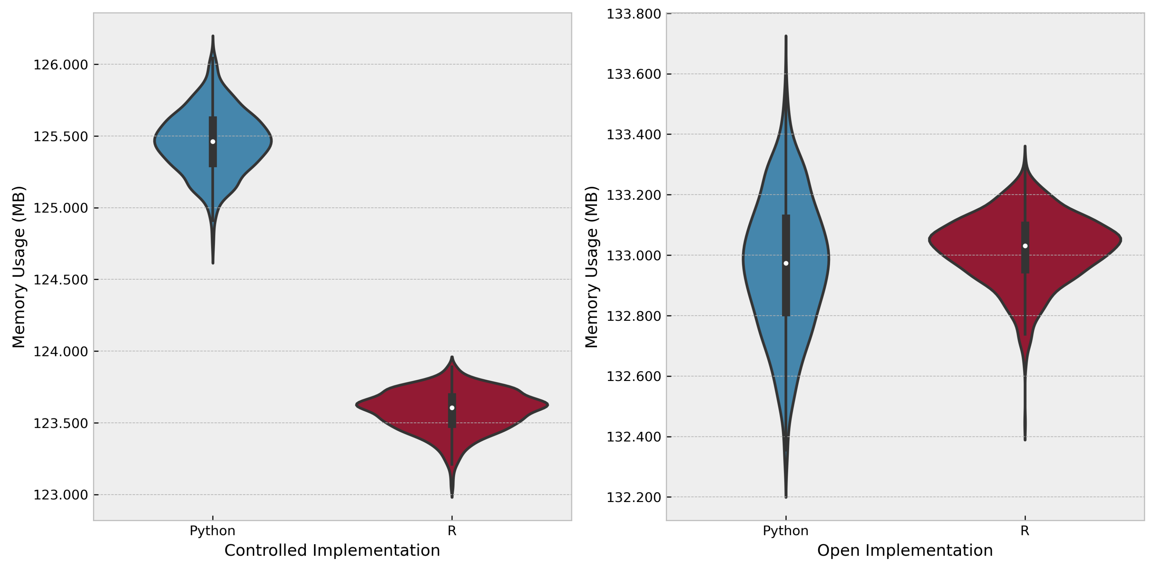
Memory usage patterns presented a contrasting narrative. In controlled systems, Python consumed slightly more memory, with a mean of 125.461 MB () compared to R’s 123.583 MB (), marking a 1.519% increase. This difference was statistically significant () with a large effect size (). However, both platforms demonstrated exceptional stability, as reflected by CV values of 0.173% for Python and 0.112% for R. These results suggest that Python’s higher baseline interpreter memory footprint accounts for the slight difference.
In open-loop systems, memory usage between the platforms converged. Python recorded a mean of 132.965 MB (), while R reached 133.020 MB (). The negligible difference of -0.042% was statistically significant (), though with a small effect size (), indicating practical equivalence. Both implementations maintained highly consistent memory utilization, with CV values below 0.2%. Figure 8, right panel, illustrates this near-parity in memory usage distributions.
Distribution shape analysis provided additional insights. Execution time data showed significant right skewness in both platforms, with Python exhibiting skewness and R exceeding 3.369 in controlled implementations. Non-normality tests (Shapiro-Wilk ) confirmed deviations from Gaussian behavior, as shown by broader tails in Figure 7. Memory usage data, on the other hand, displayed symmetric or moderately skewed distributions depending on the scenario, reflecting greater consistency in resource allocation.
Anomaly counts varied significantly across configurations. For controlled execution times, Python recorded a high anomaly rate (33.0% of data) compared to R’s 10.6%, reflecting the variability induced by Python’s dynamic optimization strategies. Conversely, in open-loop memory usage, R exhibited more anomalies (1.8%) compared to Python’s 0.4%, underscoring R’s sensitivity to subtle system conditions in memory-intensive scenarios.
Overall, Python’s execution speed makes it ideal for computationally intensive tasks, especially in controlled systems where performance is critical. However, its variability and higher anomaly rates suggest careful consideration for applications requiring extreme precision and stability. R’s strength lies in its consistent memory usage and lower variability, making it a better choice for scenarios where stability and resource predictability are paramount. These results underscore the importance of aligning platform selection with specific computational requirements to optimize performance and efficiency.
For example, Masini and Bientinesi [43] emphasizes Python’s broader ecosystem and optimization strategies as critical for scalable applications, while Raschka et al. [44] highlight R’s robustness for statistical workflows. These findings align with earlier research by Watson et al. [45], suggesting platform-specific trade-offs in computational reliability.
4. Conclusion
This study provides a comprehensive evaluation of Python and R for simulating and controlling SMD systems, with a focus on computational performance and numerical accuracy. Python exhibited a clear advantage in execution speed, achieving reductions of up to 63.57% in mean runtime compared to R in controlled system simulations. However, this efficiency came with trade-offs, including higher variability in execution times and a greater anomaly rate, reflecting the platform’s dynamic optimization strategies. Conversely, R demonstrated superior consistency in execution and memory usage, making it more suitable for scenarios prioritizing stability and resource predictability. These findings underscore the distinct strengths of each platform and the importance of selecting the right tool for specific computational needs.
The implementation of PID control significantly enhanced system dynamics, yielding improved position tracking and stability. With a final position error of just 0.4% and enhanced damping characteristics, the controlled system achieved superior performance metrics over the open-loop configuration. The controlled system’s steady-state precision and reduced settling time validate the PID controller’s design and its effectiveness in managing transient responses. Overall, this work bridges theoretical stability analysis with empirical performance insights, providing a valuable resource for researchers in computational dynamics and control systems. By leveraging the capabilities of open-source platforms, this research promotes reproducibility and transparency in the numerical study of dynamic systems.
Code and Data Availability. All code used for numerical simulations, statistical analyses, and the complete dataset generated during this study are openly available in the GitHub repository at https://github.com/sandyherho/smdCompare.
Funding. This work was supported by the Dean’s Distinguished Fellowship, University of California, Riverside, in 2023.
Declarations
Conflict of interest. The authors declare there is no conflict.
Competing interests. Authors do not have any competing financial interest to declare.
References
- Irawan, D.E.; Pourret, O.; Besançon, L.; Herho, S.H.S.; Ridlo, I.A.; Abraham, J. Post-Publication Review: The Role of Science News Outlets and Social Media. Annals of Library and Information Studies 2024, 71, 465–474. [Google Scholar] [CrossRef]
- Fraser, N.; Brierley, L.; Dey, G.; Polka, J.K.; Pálfy, M.; Nanni, F.; Coates, J.A. The evolving role of preprints in the dissemination of COVID-19 research and their impact on the science communication landscape. PLoS Biology 2021, 19, e3000959. [Google Scholar] [CrossRef] [PubMed]
- Sugimoto, C.R.; Work, S.; Larivière, V.; Haustein, S. Scholarly use of social media and altmetrics: A review of the literature. Journal of the Association for Information Science and Technology 2017, 68, 2037–2062. [Google Scholar] [CrossRef]
- Harris, C.; Millman, K.; van der Walt, S.; Gommers, R.; Virtanen, P.; Cournapeau, D.; Wieser, E.; Taylor, J.; Berg, S.; Smith, N.; et al. Array Programming with NumPy. Nature 2020, 585, 357–362. [Google Scholar] [CrossRef]
- Virtanen, P.; Gommers, R.; Oliphant, T.E.; Haberland, M.; Reddy, T.; Cournapeau, D.; Burovski, E.; Peterson, P.; Weckesser, W.; Bright, J.; et al. SciPy 1.0: Fundamental Algorithms for Scientific Computing in Python. Nature Methods 2020, 17, 261–272. [Google Scholar] [CrossRef]
- McKinney, W. Data Structures for Statistical Computing in Python. In Proceedings of the Proceedings of the 9th Python in Science Conference; pp. 201051–56. [CrossRef]
- Soetaert, K.; Petzoldt, T.; Setzer, R.W. Solving Differential Equations in R: Package deSolve. Journal of Statistical Software 2010, 33, 1–25. [Google Scholar] [CrossRef]
- Wickham, H.; Averick, M.; Bryan, J.; Chang, W.; McGowan, L.D.; François, R.; Grolemund, G.; Hayes, A.; Henry, L.; Hester, J.; et al. Welcome to the Tidyverse. Journal of Open Source Software 2019, 4, 1686. [Google Scholar] [CrossRef]
- Ogata, K. Modern Control Engineering; Prentice Hall: Upper Saddle River, NJ, USA, 2010. [Google Scholar]
- Khalil, H.K. Nonlinear Systems; Prentice Hall: Upper Saddle River, New Jersey, USA, 2002. [Google Scholar]
- Dorf, R.C.; Bishop, R.H. Modern Control Systems; Prentice Hall: Upper Saddle River, NJ, USA, 2011. [Google Scholar]
- Nise, N.S. Control Systems Engineering; John Wiley & Sons: New York City, NY, USA, 2020. [Google Scholar]
- Franklin, G.F.; Powell, J.D.; Emami-Naeini, A. Feedback Control of Dynamic Systems; Pearson: Upper Saddle River, NJ, USA, 2015. [Google Scholar]
- Åström, K.J.; Murray, R.M. Feedback Systems: An Introduction for Scientists and Engineers; Princeton University Press: Princeton, NJ, USA, 2008. [Google Scholar]
- Chen, C.T. Linear System Theory and Design; Oxford University Press: Oxford, UK, 1995. [Google Scholar]
- Waskom, M.L. Seaborn: Statistical Data Visualization. Journal of Open Source Software 2021, 6, 3021. [Google Scholar] [CrossRef]
- Georges, A.; Buytaert, D.; Eeckhout, L. Statistically Rigorous Java Performance Evaluation. ACM SIGPLAN Notices 2007, 42, 57–76. [Google Scholar] [CrossRef]
- Thompson, S.K. Sampling; Wiley Series in Probability and Statistics: New York City, NY, USA, 2012. [Google Scholar] [CrossRef]
- Herho, S.; Anwar, I.; Herho, K.; Dharma, C.; Irawan, D. COMPARING SCIENTIFIC COMPUTING ENVIRONMENTS FOR SIMULATING 2D NON-BUOYANT FLUID PARCEL TRAJECTORY UNDER INERTIAL OSCILLATION: A PRELIMINARY EDUCATIONAL STUDY. Indonesian Physical Review 2024, 7, 451–468. [Google Scholar] [CrossRef]
- Herho, S.; Fajary, F.; Herho, K.; Anwar, I.; Suwarman, R.; Irawan, D. Reappraising Double Pendulum Dynamics across Multiple Computational Platforms. Preprints 2024. [Google Scholar] [CrossRef]
- Herho, S.; Kaban, S.N.; Irawan, D.E.; Kapid, R. Efficient 1D Heat Equation Solver: Leveraging Numba in Python. Eksakta : Berkala Ilmiah Bidang MIPA. [CrossRef]
- Jain, R. The Art of Computer Systems Performance Analysis: Techniques for Experimental Design, Measurement, Simulation, and Modeling; John Wiley & Sons: New York, USA, 1991. [Google Scholar]
- Brown, R.J.C.; Brown, R.F.C. Statistical Analysis of Measurement Data; Royal Society of Chemistry: London, United Kingdom, 1998. [Google Scholar]
- Hoaglin, D.C.; Mosteller, F.; Tukey, J.W. Understanding Robust and Exploratory Data Analysis; Wiley-Interscience: Hoboken, NJ, USA, 2000. [Google Scholar]
- Mostafavi, S.; Hakami, V.; Paydar, F. Performance Evaluation of Software-Defined Networking Controllers: A Comparative Study. Computer and Knowledge Engineering 2020, 2, 63–73. [Google Scholar] [CrossRef]
- Montgomery, D.C. Design and Analysis of Experiments; John Wiley & Sons: New York City, NY, USA, 2017. [Google Scholar]
- Bulmer, M.G. Principles of Statistics; Dover Publications: New York, USA, 1979. [Google Scholar]
- Razali, N.M.; Wah, Y.B. Power Comparisons of Shapiro-Wilk, Kolmogorov-Smirnov, Lilliefors and Anderson-Darling Tests. Journal of Statistical Modeling and Analytics 2011, 2, 21–33. [Google Scholar]
- Siegel, S. Nonparametric Statistics for the Behavioral Sciences; McGraw-Hill: New York City, NY, USA, 1956. [Google Scholar]
- Wilcoxon, F. Individual Comparisons by Ranking Methods. Biometrics Bulletin 1945, 1, 80–83. [Google Scholar] [CrossRef]
- Levene, H. Robust Tests for Equality of Variances. In Contributions to Probability and Statistics; Olkin, I., Ed.; Stanford University Press: Stanford, California, USA, 1960; pp. 278–292. [Google Scholar]
- Brown, M.B.; Forsythe, A.B. Robust Tests for the Equality of Variances. Journal of the American Statistical Association 1974, 69, 364–367. [Google Scholar] [CrossRef]
- Sullivan, G.M.; Feinn, R. Using Effect Size—or Why the P Value is Not Enough. Journal of Graduate Medical Education 2012, 4, 279–282. [Google Scholar] [CrossRef]
- Cohen, J. Statistical Power Analysis for the Behavioral Sciences; Routledge: New York City, NY, USA, 1988. [Google Scholar] [CrossRef]
- Sawilowsky, S.S. New Effect Size Rules of Thumb. Journal of Modern Applied Statistical Methods 2009, 8, 597–599. [Google Scholar] [CrossRef]
- Iglewicz, B.; Hoaglin, D.C. Volume 16: How to Detect and Handle Outliers; ASQC Quality Press: Milwaukee, WI, USA, 1993. [Google Scholar]
- Chandola, V.; Banerjee, A.; Kumar, V. Anomaly Detection: A Survey. ACM Computing Surveys 2009, 41, 1–58. [Google Scholar] [CrossRef]
- Rousseeuw, P.J.; Croux, C. Alternatives to the Median Absolute Deviation. Journal of the American Statistical Association 1993, 88, 1273–1283. [Google Scholar] [CrossRef]
- Tukey, J.W. Exploratory Data Analysis; Addison-Wesley: Reading, MA, USA, 1977. [Google Scholar]
- Aggarwal, C.C. Outlier Analysis; Springer: New York City, NY, USA, 2013. [Google Scholar] [CrossRef]
- Mytkowicz, T.; Diwan, A.; Hauswirth, M.; Sweeney, P.F. Producing Wrong Data Without Doing Anything Obviously Wrong! ACM SIGARCH Computer Architecture News 2009, 37, 265–276. [Google Scholar] [CrossRef]
- Altman, D.G.; Machin, D.; Bryant, T.N.; Gardner, M.J. Statistics with Confidence: Confidence Intervals and Statistical Guidelines; BMJ Books: London, UK, 2013. [Google Scholar]
- Masini, S.; Bientinesi, P. High-Performance Parallel Computations Using Python as High-Level Language. In Proceedings of the Euro-Par 2010 Parallel Processing Workshops; Guarracino, M.R.; Vivien, F.; Träff, J.L.; Cannatoro, M.; Danelutto, M.; Hast, A.; Perla, F.; Knüpfer, A.; Di Martino, B.; Alexander, M., Eds., Berlin, Heidelberg; 2011; pp. 541–548. [Google Scholar] [CrossRef]
- Raschka, S.; Patterson, J.; Nolet, C. Machine Learning in Python: Main Developments and Technology Trends in Data Science, Machine Learning, and Artificial Intelligence. Information 2020, 11, 193. [Google Scholar] [CrossRef]
- Watson, A.; Babu, D.S.V.; Ray, S. Sanzu: A data science benchmark. In Proceedings of the 2017 IEEE International Conference on Big Data (Big Data); 2017; pp. 263–272. [Google Scholar] [CrossRef]
Figure 1.
Physical representation of the idealized SMD system showing coordinate system and force components. The origin was set at the spring’s equilibrium position, with positive displacement defined in the rightward direction.
Figure 1.
Physical representation of the idealized SMD system showing coordinate system and force components. The origin was set at the spring’s equilibrium position, with positive displacement defined in the rightward direction.
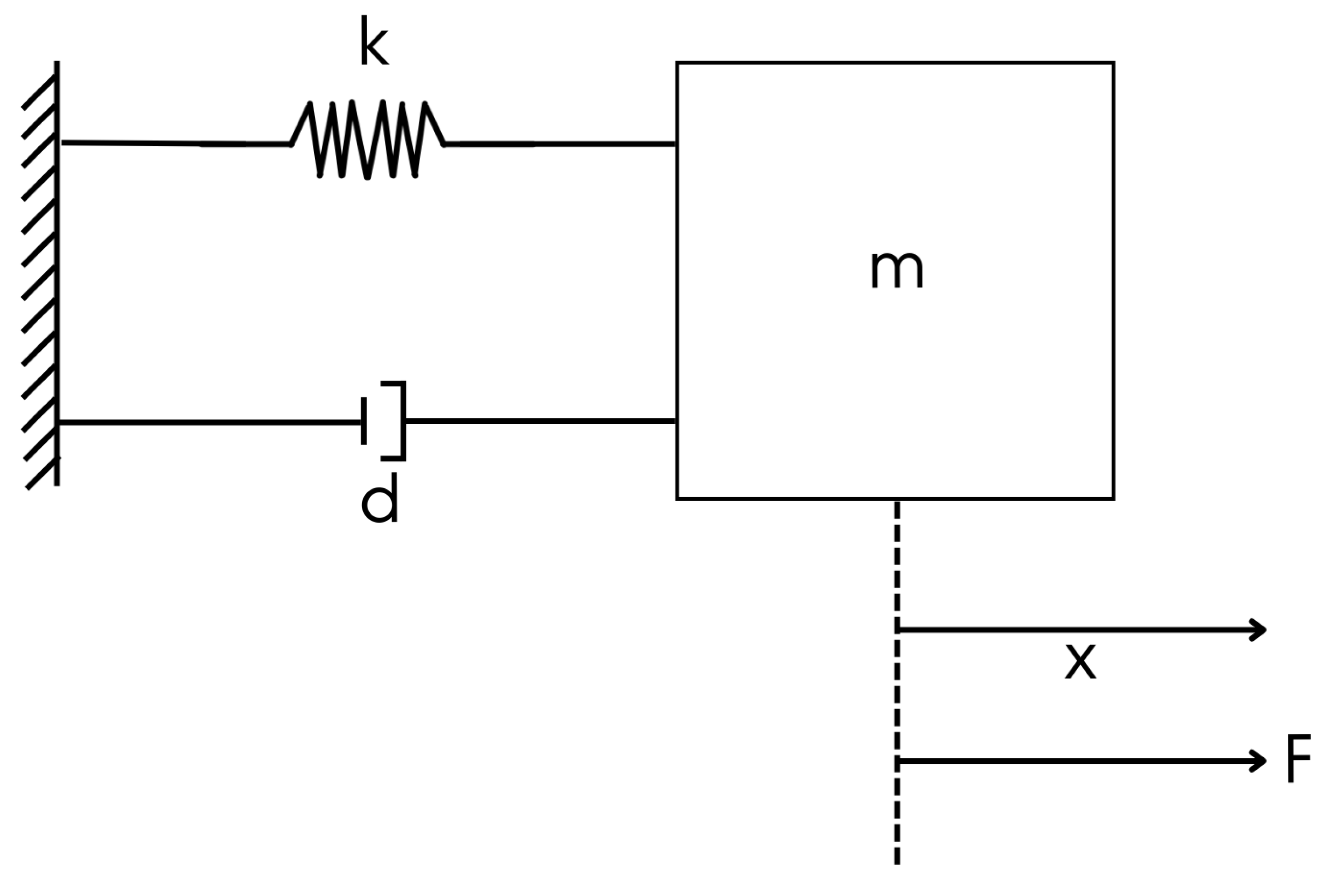
Figure 2.
Block diagram representation of the SMD system: Open-loop configuration showing direct force input with system transfer function and closed-loop configuration illustrating PID control architecture with complete signal flow paths and transfer functions.
Figure 2.
Block diagram representation of the SMD system: Open-loop configuration showing direct force input with system transfer function and closed-loop configuration illustrating PID control architecture with complete signal flow paths and transfer functions.
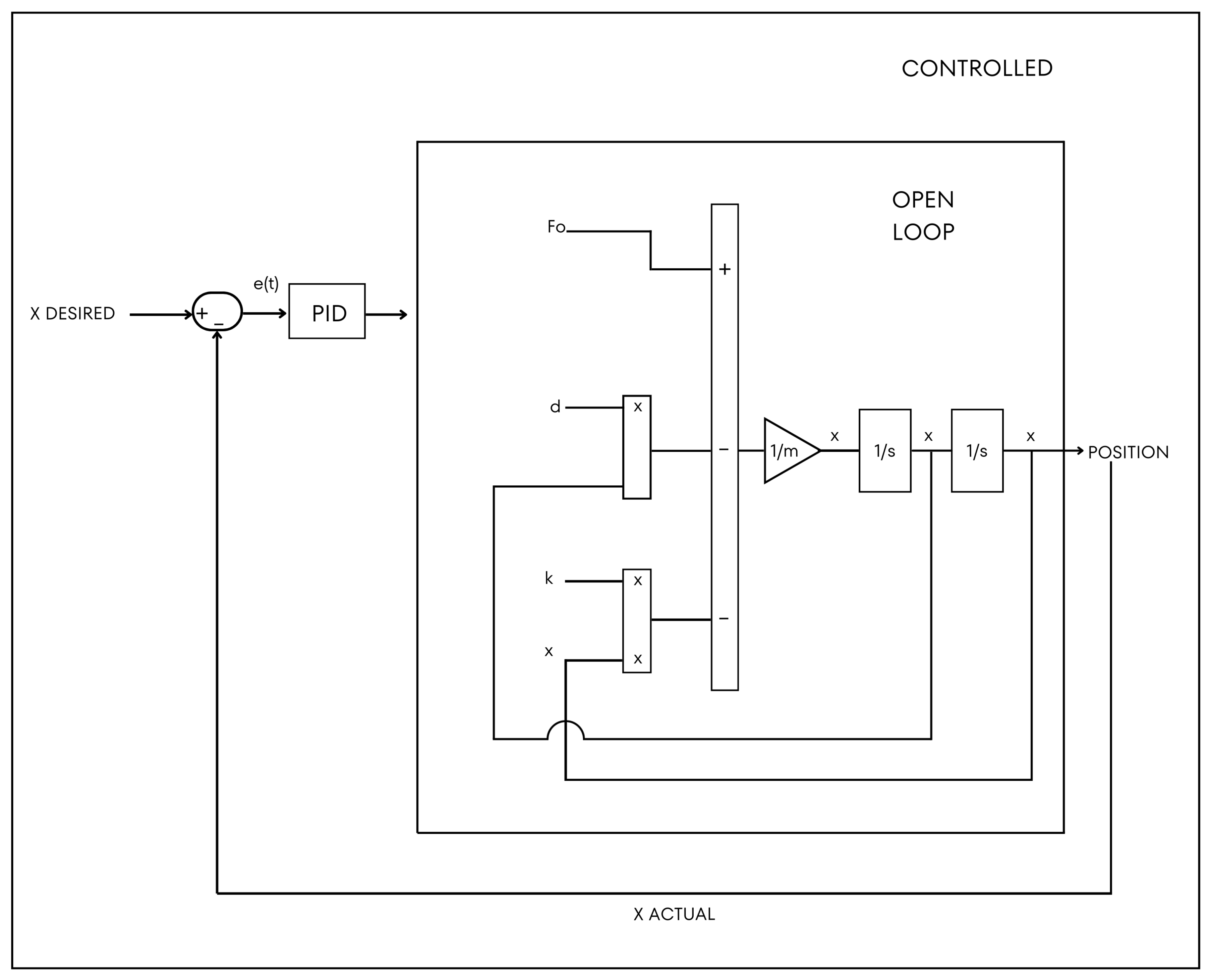
Figure 3.
Temporal evolution of the open-loop system response to a 50 N step input. From top to bottom: (a) Applied force showing the transition from 0 to 50 N between t = 4 s and t = 5 s, (b) Position response demonstrating underdamped oscillations converging to 1.000 m, (c) Velocity profile reaching a maximum of 0.4 m/s before dampened oscillations to zero, and (d) Acceleration response highlighting the system’s dynamic behavior with peak values of ± 0.2 m/s2.
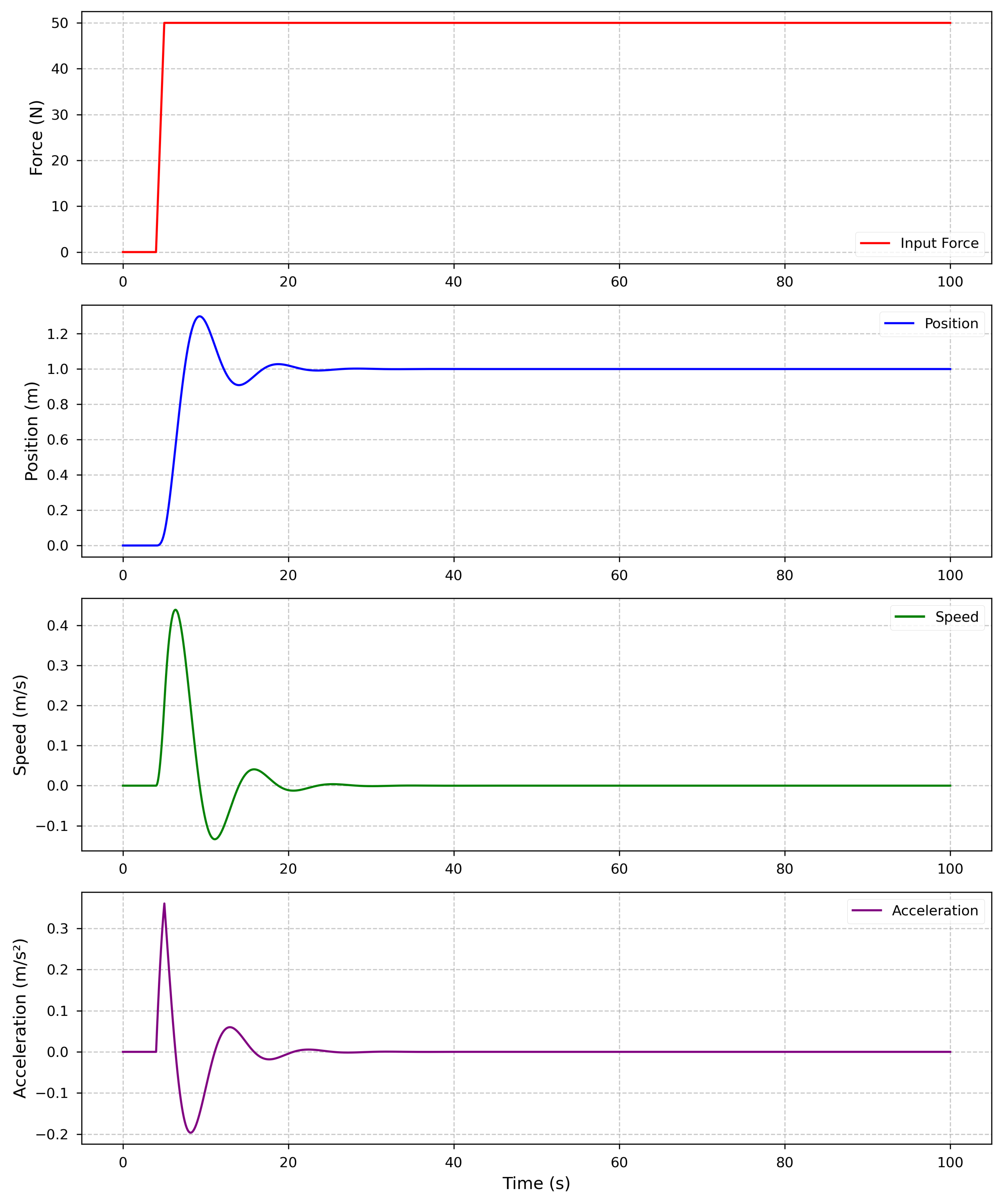
Figure 4.
Phase portrait of the open-loop system showing the relationship between position and velocity. The spiral trajectory, beginning from the origin and converging to the equilibrium point (1 m, 0 m/s), illustrates the system’s stable focus behavior. The decreasing spiral radius demonstrates the energy dissipation through damping, while the elliptical shape reflects the interchange between potential and kinetic energy.
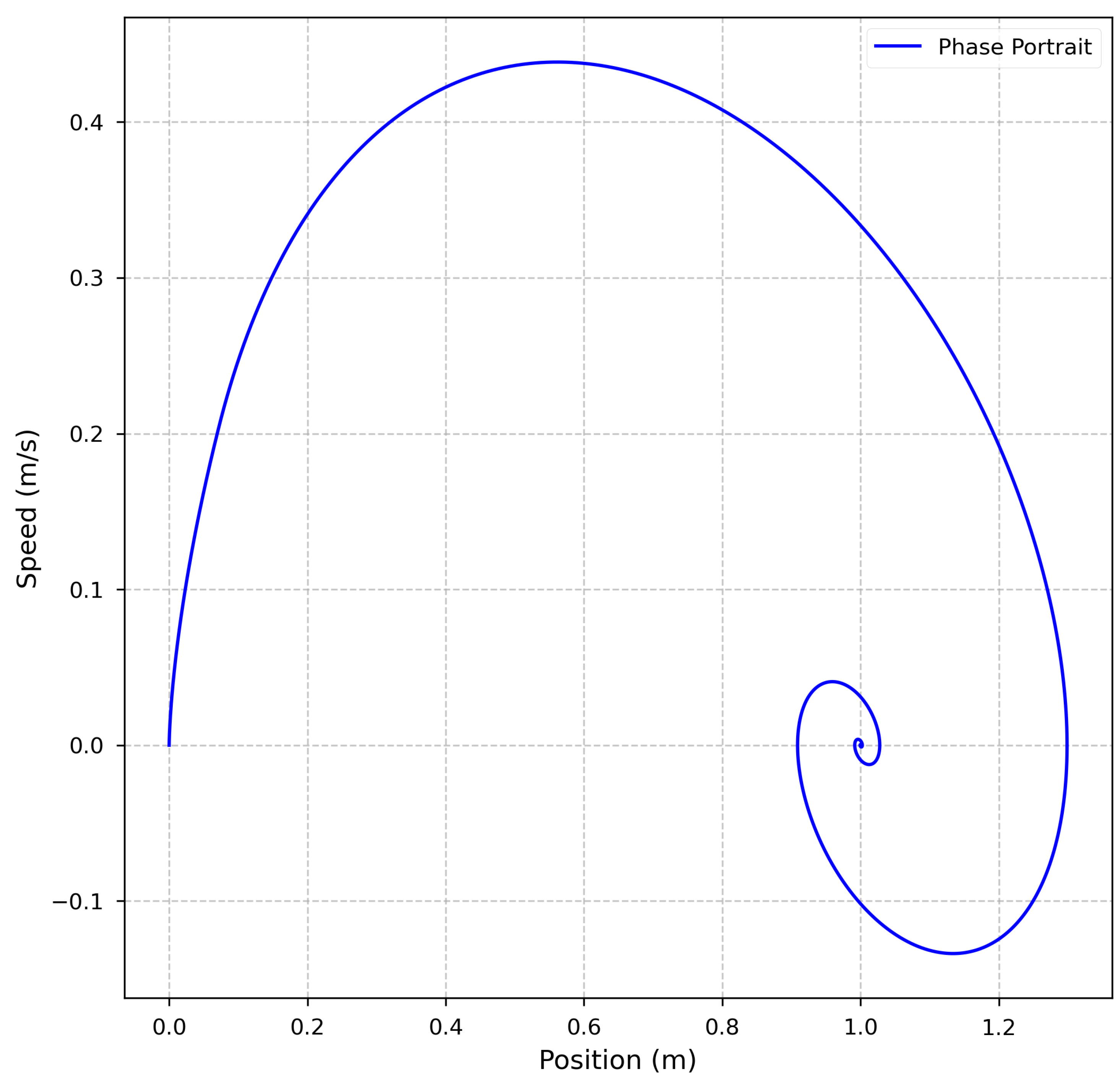
Figure 5.
Closed-loop system response with PID control. From top to bottom: (a) Position tracking showing desired (dashed red) and actual (solid blue) trajectories, demonstrating effective reference tracking, (b) Control force profile exhibiting initial peak of 259.2 N followed by smooth regulation, (c) Position error evolution showing maximum deviation of 0.107 m and final error of 0.004 m, (d) Velocity response with peak of 1.04 m/s, and (e) Acceleration profile with maximum of 2.14 m/s2.
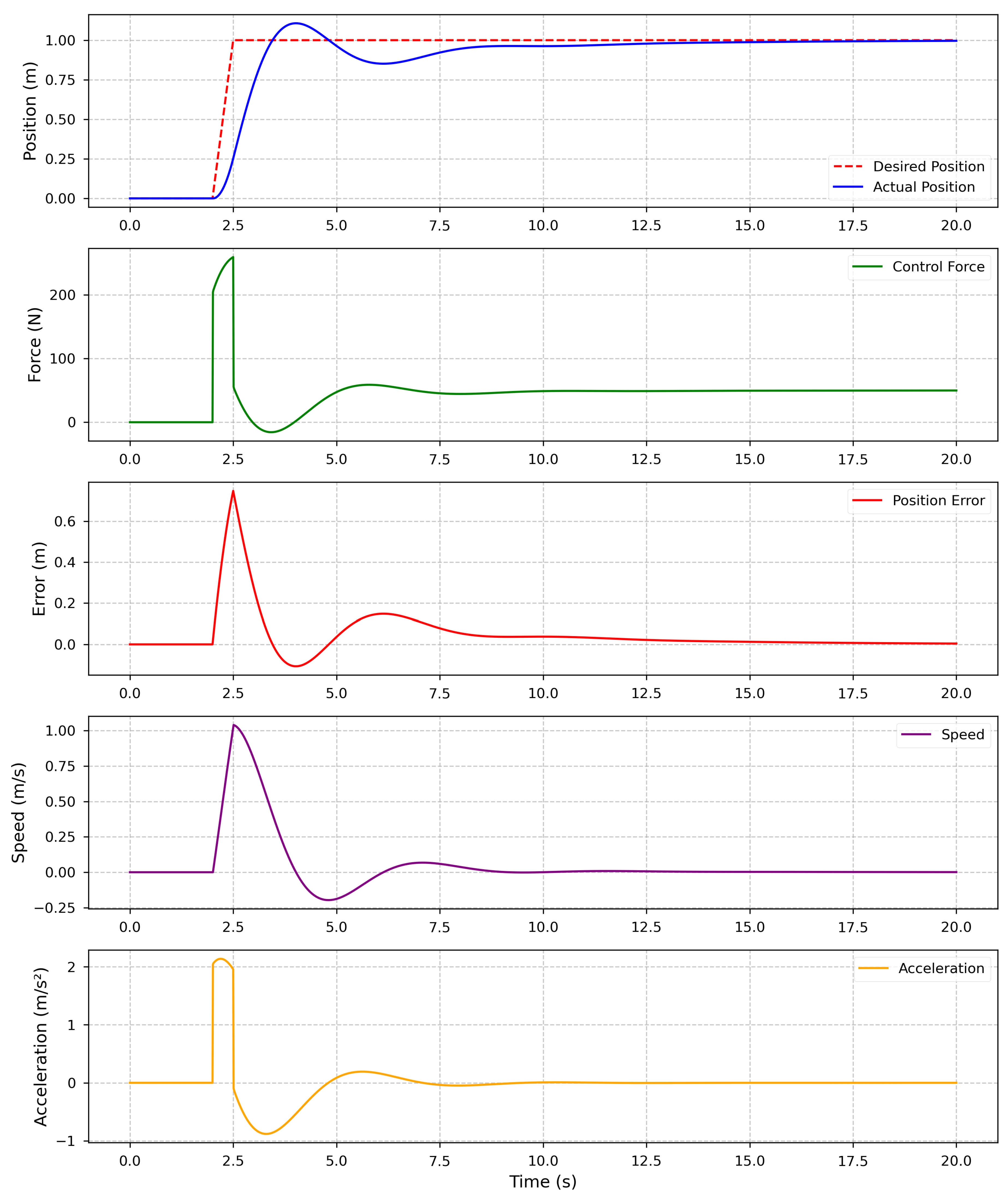
Figure 6.
Phase portrait of the closed-loop system illustrating the controlled state-space trajectory. The smooth path from initial conditions to the desired setpoint (1.0 m, 0 m/s) demonstrates the controller’s ability to regulate both position and velocity simultaneously. The absence of multiple spirals indicates improved damping compared to the open-loop response.
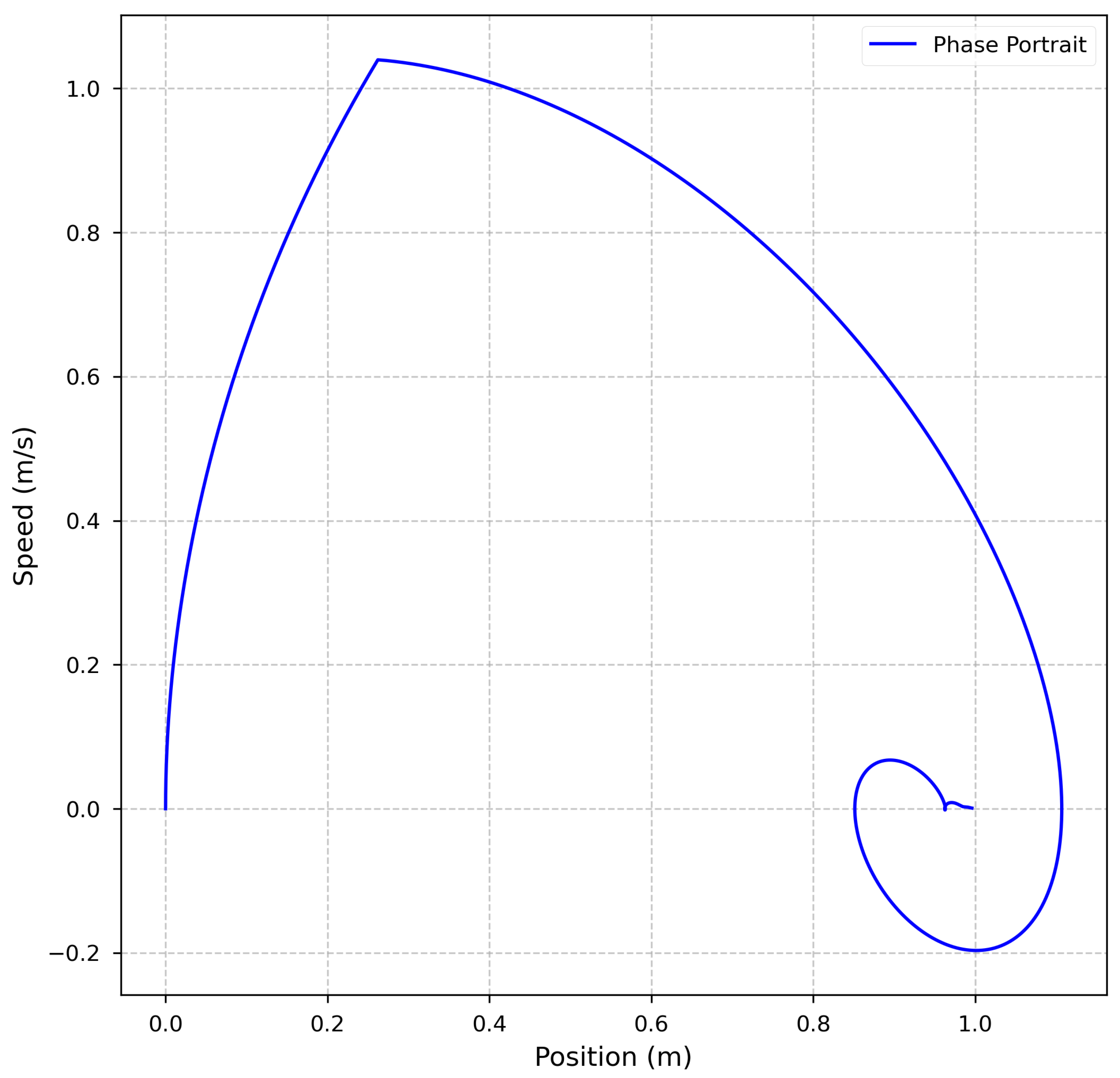
Figure 7.
Violin plots of execution time distributions for Python and R under controlled and open-loop implementations. The left panel represents controlled implementations, while the right panel shows open-loop implementations.
Figure 7.
Violin plots of execution time distributions for Python and R under controlled and open-loop implementations. The left panel represents controlled implementations, while the right panel shows open-loop implementations.
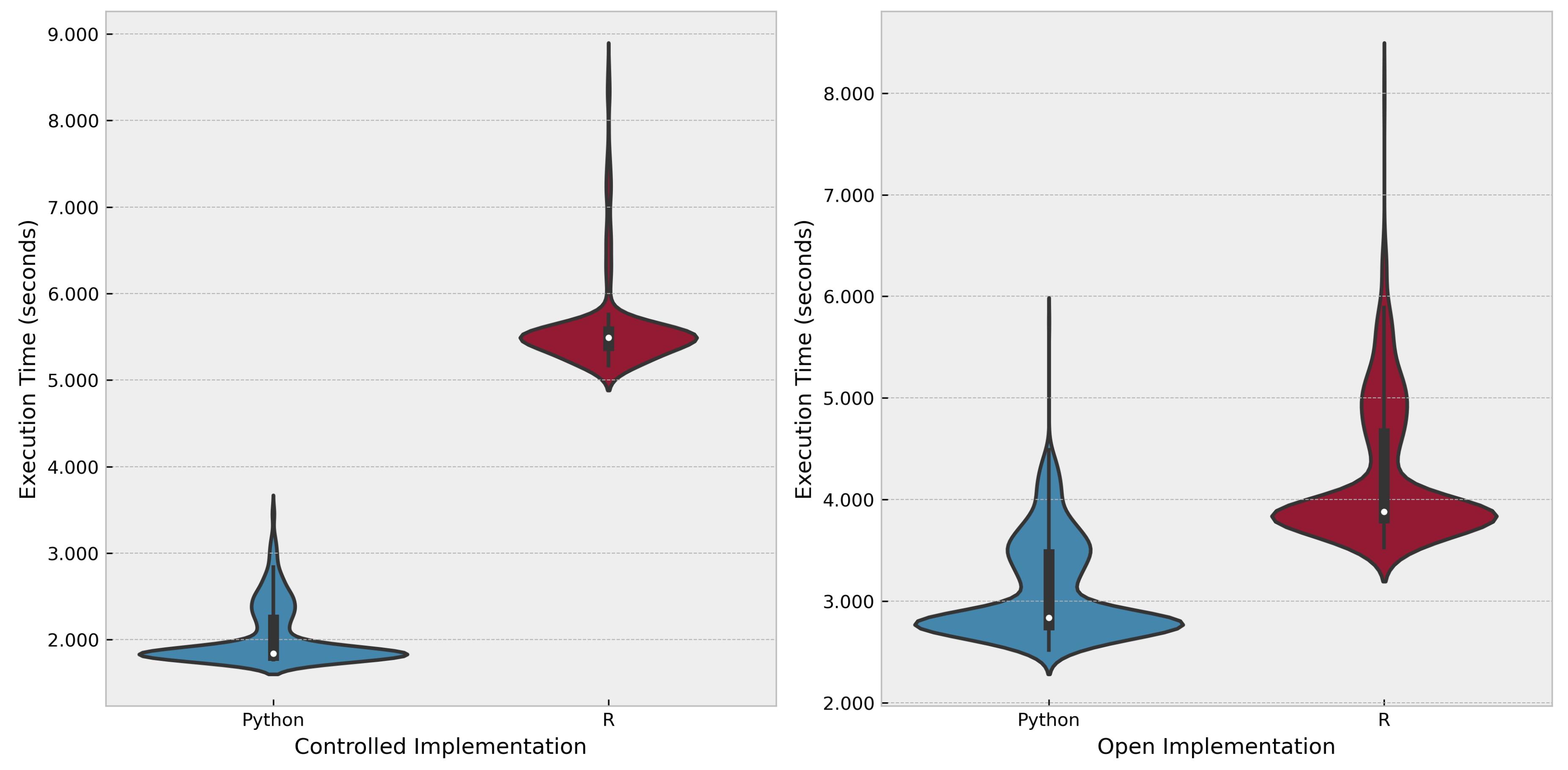
Figure 8.
Violin plots of memory usage distributions for Python and R under controlled and open-loop implementations. The left panel represents controlled implementations, while the right panel shows open-loop implementations.
Figure 8.
Violin plots of memory usage distributions for Python and R under controlled and open-loop implementations. The left panel represents controlled implementations, while the right panel shows open-loop implementations.
Disclaimer/Publisher’s Note: The statements, opinions and data contained in all publications are solely those of the individual author(s) and contributor(s) and not of MDPI and/or the editor(s). MDPI and/or the editor(s) disclaim responsibility for any injury to people or property resulting from any ideas, methods, instructions or products referred to in the content. |
© 2025 by the authors. Licensee MDPI, Basel, Switzerland. This article is an open access article distributed under the terms and conditions of the Creative Commons Attribution (CC BY) license (https://creativecommons.org/licenses/by/4.0/).
Copyright: This open access article is published under a Creative Commons CC BY 4.0 license, which permit the free download, distribution, and reuse, provided that the author and preprint are cited in any reuse.


