
Submitted:
27 December 2024
Posted:
30 December 2024
You are already at the latest version
Abstract
In this paper, we propose a new geometric-shaping design for golden angle modulation (GAM) based on the complex geometric properties of open symmetrized bidisc, termed Bd-GAM, for future generation wireless communication systems. Inspired from the circular symmetric structure of the GAM, we construct the modulation schemes, Bd-GAM1 and Bd-GAM2. However, the optimization problem is hard to solve analytically, we consider this problem in the domain of symmetrized bidisc. Specifically, we joint the complex geometrics properties of symmetric bidisc and MI-optimized probabilistic modulation scheme. The symmetric bidisc is a bounded domain on which the Carathe´odory distance and the Kobayashi distance coincide. We can use the pseudo-metric mD in unit disc D to get the Kobayashi pseudo-distance and Carathe´odory pseudo-distance. With minimum SNR and entropy constraint, Bd-GAM1 and Bd-GAM2 can overcome the shaping-loss. This study finds that each constellation point of Bd-GAM has a unique phase and gain. Compared with the existed golden angle modulation introduced, the new design improves the mutual informaiton (MI), and the distance between adjacent constellation points.
Keywords:
shannon-Hartley theorem
; mutual information
; symmetric bidisc
; golden modulaiton
; geometric shaping
; pseudoconvex domain
MSC: 94A14
1. Introduction
To further achieve spectral resources and provide high rate data transmission, the application of constellation shaping in most existed modulation schemes have finite-dimension constellations. Phase shift keying (PSK), amplitude PSK (APSK) [1], star-QAM [2] and square/rectangular-QAM have been analyzed. QAM has 1.53 dB) SNR gap between the mutual information (MI) and the additive white Gaussian noise (AWGN) capacity [3]. Geometric- and probabilistic- shaping were considered to overcome the shaping loss. The research of this problem are nonuniform QAM [4,5] and PSK [6] capacity optimization. In [7,8,9], there are some works about probabilistic shaping. In [10] and [11], trellis shaping and shell shaping were proposed on probabilistic shaping. Geometric shaping with circular symmetry (i.e. APSK) is an effective method to get (complex Gaussian) distribution. However, the number of constellation points in each orbit (or ring) depend on the geometric shaping of some modulation. Recently, [12,13,14] introduced a new framework inspired by Vogel [15]. [12,13] mainly proposed Disc-GAM, Geometric Bell-GAM (GB-GAM), geometric-GAM and probabilistic-GAM. As the core features of GAM, the golden angle in the phase domain and the radial/phase distribution of constellation points were introduced. On the orbit (or ring), the constellation point of Bd-GAM is located so that the angular distance between two adjacent points must be equal to a golden angle . In [12,13], the MI of GB-GAM is close to the channel capacity,i.e. , where H is the constellation entropy. However, neither GB-GAM, nor Disc-GAM can get a good MI performance over a wide SNR range. [14] has solved a numerical optimization problem to maximize the MI for every SNR by optimizing the radius . Finally, [14] proposed a Truncated Geometric Bell-shaped GAM and solved the optimization problem by classical Lagrangian optimization. At the same time, the numerical optimization problem, maximize the MI for any SNR, can be handled by parameterizing the analytical magnitude expression such that the MI can be improved for a wide SNR range. The MI performance of the new design in [14] is better than other designs, i.e. GB-GAM, disc-GAM and QAM.
We note that few works of GAM consider the complex geometric properties in the domain. Pseudoconvex domain is a fundamental concept in the classical function theory of several complex variables [16]. Let be the symmetrized bidisc, which is the image of bidisc , namely . The open symmetrized bidisc [17] has attracted more interests in Engineering Mathematics and Complex Analysis such as the spectral Nevanlinna-Pick interpolation problem. Inspired by the novel modulation shceme (GAM) and complex geometric properties, the golden angle modulation based on the symmetrized bidisc (Bd-GAM) is introduced. Notice that, the so-called Poincar distance can be provided by . Poincar disc model is built up in the Euclidean plane. The distance between constellation points is defined in Euclidean geometry [12,13,14]. In this paper, we will expand the study on geometric-shaping and provide the performance analysis to Bd-GAM on .
The main contributions of this paper can be summarized as follows: 1) Two new modulation cases of Bd-GAM1 and Bd-GAM2 have been presented. 2) Under the ’symmetrization map’, the unit disc is transformed into the symmetrized bidisc on . The complex numerical optimization of MI metric allows larger constellation sizes on . 3) For the optimization formulation, the discrete format of complex numerical optimization is derived. We present the Monte Carlo simulation results of MI-performance with Bd-GAM.
The rest of this paper is organized as follows. In Section 2, we recall some related works about the GAM, as well as complex geometric properties of symmetrized bidisc. Section 3 presents the optimization problem of MI performance, arising from the constellation points of Bd-GAM. Considering the complex numerical optimization of MI, we further modify the complex integration with discrete format. Seciton 4 provides a MI performance simulations for the Bd-GAM1/2. The performance of the Bd-GAM is evaluated by means of Monte Carlo simulations. The paper is concluded in Section 5.
2. Related Works
2.1. Golden Angle Modulation on
Golden Angle Modulation (GAM) [12] is a recently designed modulation scheme, which can provide enhanced MI and PAPR performance over QAM. This modulation scheme can be applied to a wide range of research fields, such as wireless, optical and communication systems. [18] proposed a new method to design SCMA codebooks based on the GAM [12] for downlink and uplink SCMA systems. In [20], quantizers based on the GAM [12] were proposed. The quantizer shceme provides an effective design and any number of centroids.
Consider the metric property of the unit disc itself on , the basic definition for unstructured GAM modulation in [12] is
where is the radius of n- constellation point and is the golden angle, where . If is an increasing spiral winding with and , then . Moreover, for the probability of each constellation point, we have and , which is dependent on index n. [14] generalized the Disc-GAM and defined as follows:
where is average power. This design is a punctured unit disk. is the number of inner constellation points in the hole. is the total number of points in the unit disk. The probability of the n- constellation point is ().
The corresponding constellation of normalized GAM is in Figure 1. The first row of Figure 1 is the Disc-GAM [12], obtained with Eq. (1) - Eq. (3) as the number of constellation points are . The second row of Figure 1 is the Generalized Disc-GAM with Eq. (4) - Eq. (6) as the number of constellation points are . The design of constellation points is spiral phyllotaxis. There is enough distance between adjacent constellation points for blind estimation based on decision method.
Figure 2 depicts the constellation of normalized Disc-GAM vs. SNR. The first row is the Disc-GAM with and SNR = 10 dB. The other rows are the Disc-GAM with and SNR dB, 35 dB}. For the last column, the signal constellation magnitudes have the same distribution as complex Gaussian for low SNRs, and the same distribution as uniform unit disc for high SNRs.
Geometric Bell-Golden Angle Modulation [12] was induced by the inverse sampling method and approximates a complex Gaussian distribution. It is defined as follows:
where N is the number of constellation points. is the average power normalization constraint. is the complex amplitude of the th constellation point. The corresponding constellation of normalized GAM is in Figure 3 with . From this figure, one can observe that most of the constellation points are dense around the center and the center point is the pdf-peak-point of the Gaussian distribution.
In Table 1, we present in a unified way entropy and PAPR of five different modulation methods. Disc-GAM has better PAPR performance than QAM, while QAM has 1.53 dB SNR-gap to the AWGN Shannon capacity [3]. Here, PSK has PAPR dB with poor MI-performance. From entropy-point of view, the Disc-GAM is a special design of generalized Disc-GAM with punctured unit disk.
2.2. Complex Geometric Properties of Open Symmetrized Bidisc
In this section, we review some basic properties of open symmetrized bidisc. For the open unit disc in , the open symmetrized bidisc is the image of the bidisc under the `symmetrization map’, namely
where . Meanwhile, is not biholomorphic to any convex domain in [20]. is a bounded domain on which the Kobayashi distance and the Carathodory distance coincide. By definition [21], we can get the Carathodory pseudo-distance between any point and as follows
where the supremum is defined accroding to all analytic functions
and d denotes the hyperbolic distance on . Note that, is holomorphic for any in . Moreover, for the Lempert function in and pseudo-metric in , we have defined
Then we can get the Kobayashi pseudo-distance as follows
Let d denotes the hyperbolic distance on . We have
The analytic function is a complex geodesic on if and only if . For any , we have
There exists an analytic function such that , for all . By definition, we know that the Kobayashi pseudo-distance (Eq. (13)) on is the largest pseudo-distance, but smaller than . Then we have the following relation
In particular, from the definition of , we can find that as any point of unit disc can be moved biholomorphically to any other point of unit disc. S is the possibly smallest , such that there exists an analytic funciton satisfying . Finally, we recall that the complex geodesics of open symmetrized bidisc is the solutions of the Kobayashi extremal problem [17], which implies that
Notice, Eq. (17) is true for general convex domain in [22]. is not biholomorphic to any convex set in , but the Carathodory pseudo-distance on coincide with Lempert function. For the definition of the Kobayashi (pseudo) distance, we observe that the Kobayashi distance coincides with the Poincar distance in the unit disc. Thus, the Kobayashi (pseudo) distance on can be larger than the Poincar distance in the Euclidean plane, because the Poincar distance coincides with . These properties can enhance the distance between adjacent constellation points and allow better natural constellation point index order. Meanwhile, is a bounded pseudoconvex domain. By altering some homogeneous plurisubharmonic polynomial of radius , we can solve the complex optimization problem. An complex analysis method can be used to design the modulation. We also note that few works of GAM consider the complex geometric properties of the domain.
3. GAM on the Symmetrized Bidisc
In Table 1, the entropy and PAPR of GAM in are and dB (). The power normalization of original constellation point is . Compared to 2 dB for GAM on , the peak-to-average SNR Ratio is 1 dB for Bd-GAM on . The design generalize the GAM to higher dimensions in complex space.
3.1. Bd-GAM1
Let . With the definition of , we have
Denote , and . As the average power of constellation points is a constraint, there is
3.1: Let . is a constant, i.e., . Notice that
Let . We have . Since the root of equation is the set , we know the root of equation is the set . With the Vitea theorem, we obtain
Then we get .
3.2: is bounded as the number of constellation points N are not infinite. In fact, . The series is bounded as N is not infinite. The boundary is shown in Figure 4. The upper bound and lower bound are often a good constraint of c2.
From 3.1 and 3.2, we show that is bounded. This makes the Bd-GAM possible with higher dimensions. Compared with in [12,13,14], Bd-GAM1 can alter the value based on the complex variable and the number of points. Meanwhile, the amplitude is . As depends on and N, the following MI optimization problem can be solved without the limitation of constellation size.
Figure 5 shows the normalized Bd-GAM1 signal constellation with different points. The left part (red box) of this figure is the original image set, denoted by . The right region (blue box) is the image set under . The In-phase and Quadrature of signal are and . Then we have , where . is the inverse mapping set. Note that it is denset at the bottom of bell.
3.2. Bd-GAM2
Let . With the definition of , we have
Denote . The average power of constellation points is
Set . The corresponding constellation of Bd-GAM2 is Figure 6. The left part (red box) of this figure is the original image set, denoted by . The right region (blue box) is the image set under . Then we have . is the inverse mapping set. Note that it is a circular design, which can offer enhanced MI- and distance performance over GAM and square-QAM design.
3.3. MI Optimization Problem of Probabilistic- and Geometric- Bd-GAM: Bd-GAM1/2
Let N be the number of constellation points. is the probability for each constellation point. Similar to method [12], Bd-GAM1/2 can control the radius to maximize the MI. It is a difference that the proposed methods can synchronously select the radius and phase by optimizing just a variable . With this method, we optimize that maximizes the MI for a given SNR. In the region , the optimized n-th signal constellation point is . Denote the complex valued output by r.v. Y. The complex valued input with discrete modulation is r.v. Z. Then we have the following MI-optimization problem
In the above, the mutual information I can be expressed with terms i.e. the differential entropy and conditional differential entropy . Meanwhile, we have , where . integrates in the complex domain and
With Eq. (24), we can get the discrete formation of as follows
In Eq. (25), we put , , the sum of the series and . Then we have
For and , we can write for . The baseband samples are . The bivariate conditional pdf is . Without loss of generality, we let tangent vector and boundary point here. Calculations lead to the following formula:
Similarly, we have
Let the average power of the signal be normalized and the noise variance is . We also have the discrete formation. It follows that
For the output Y, the Levi form is
By Eq. (26) and Eq. (29), semi-positive definiteness of Eq. (30) can be verfied. It suffices to prove that the region of the signal constellation points is a pseudoconvex domain. Then we can find some function to design the radius in the region. The densest point at the center, i.e. where the pdf for the complex Gaussian r.v. peaks, is a peak point relative to if there is a holomorphic funtion f satisfying and for all .
4. Numerical Results and Discussions
4.1. The Complex Geometric Properties Analysis of Bd-GAM1/2
In this part, we present the Bd-GAM signal constellation in Figure 7. Each modulation signal points of Bd-GAM are labeled with the same color as their labels (i.e. n-ord F1/F2 stand for Bd-GAM1/2 with ). We note that the shapes of Bd-GAM2 constellation expand as the modulations increase from 2 to 10. Compared with Bd-GAM2, the geometric shaping of Bd-GAM1 is symmetric and the boundary points shrink toward the center as the modulation N increases. The inner points fill the interior of the bell along the direction of the tangent vector. In contrast to GAM, with natural constellation point indexing, the proposed Bd-GAM can provide enhanced distance performance. In the following, we plot the orbit for the points of the Bd-GAM signal constellation.
Figure 8 plots the orbit for each modulation signal. The left part of this figure is the orbit for the symmetric center of Bd-GAM1. The orbit of the constellatio points becomes more flattened as the radius increases. Meanwhile, the orbit for the boundary points of Bd-GAM2 expands with spiral phyllotaxis packing.
4.2. Magnitude Distribution of Bd-GAM1
In Figure 9, we plot the magnitude distribution of Bd-GAM1 with different constellation points (i.e. ). Without noise, the first column of this figure presents the magnitude distribution for constellation points in (denoted as sym-disc-in-C2) and points in (denoted as disc-in-C1). We observe that the signal constellation magnitudes of `sym-disc-in-C2’ are larger than magnitudes of `disc-in-C1’. The middle column of it is the magnitude distribution with SNR = 22.5 dB. In the eighth subplot, we can see that there exist some little oscillatory problem for the initial constellation points. The last column contains three subplots of magnitude distribution for constellation points in (denoted by sym-disc-in-G2/sym-noisy-disc-in-G2). Let `sym-noisy-disc-in-G2’ stand for the one with SNR = 22.5dB and `sym-disc-in-G2’ is the case without noise. Clearly, we can see that Bd-GAM1 has a stable magnitude distribution and good ability to overcome the noise.
4.3. Kobayashi Pseudo-Distance of Adjacent Constellation Points
In Figure 10, we illustrate the distance-performance for the Bd-GAM2 in with hyper-distance in and distance in Euclidean plane. The constellation size is and SNR = 22.5 dB. Select the front fifteen constellation points and calculate the distance between these points with other 255 constellation points over different domains (e.g. , , and ). Note that the distance for the adjacent points in is always larger than the distance for the points of unit disc in Euclidean plane. These constellation points keep relatively natural index order and the radial distribution of constellation points can be tuned. This avoids regions overlapping, such as phase/amplitude region. With the MI optimization problem, it is important to ensure the distance between adjacent constellation points as the modulation N increases. However, compared with the distance in , the distances of Bd-GAM2 in decrease. The reason is that the constellation points are designed along the orbit of the boundary points. Thus, a part of constellation points (or boundary points) may have phase drift or rotation under the holomorphic mapping f. At the same time, this phenomenon can solve the geometric problem (i.e. the analytic of the expression for ) for the siganl constellation points. When the complex geometric properties, MI and power constraints are included, the inner constellation points in are designed by Bd-GAM1 method. Using the geometric and probalilistic -shaping, we assume the signal constellation design with and let be the pmf to find the optimal scheme for constellation points.
4.4. Mutual Information Performance for Bd-GAM
In this section, we present the MI-performance of Bd-GAM1/2. Monte-Carlo simulations of the MI-performance curves are used. The MI estimator [14] is defined by
where K is the number of iterations. z is randomly produced by with .
A. Bd-GAM1
In Figure 11, we compare two different modulation methods, Bd-GAM1 [12,13] and QAM, with the AWGN Shannon capacity. The complex numerical integration is deduced in section 3.3. The corresponding formulas are Eq. (25) and Eq. (26). We can use Eq. (27) - Eq. (30) to determine the orbit of the constellation points with some geometric and probalilistic -shaping. As expected, there exists a greater overlap with the AWGN Shannon capacity when the constellation points increase.
Compared with Disc-GAM [12,13] method, Bd-GAM1 have nearly the same MI-performance as the AWGN Shannon capacity for low SNRs, and better MI-performance than Disc-GAM for high SNRs. Meanwhile, Bd-GAM1 can overcome the oscillatory phenomenon of magnitude distribution for low SNRs. The constellation size is twice that of the Disc-GAM and the additional energy consumption is required. But these costs are of less concren and in exchange for more MI-performance. Thus the Bd-GAM1 is a better optimizaiton framework, maximizing the MI under the SNR constraint.
B. Bd-GAM2
In Figure 12, we illustrate the MI-performance for the Bd-GAM2 together with the AWGN Shannon capacity. This design implies that and we find that is suitable for Bd-GAM2. There exists a potential advantage for the geometric-shaping and probabilistic-shaping (i.e. entropy H and pmf are fixed for a given N). Note that, when the MI approaches the entropy, Bd-GAM2 performs better than QAM method. Thus, Bd-GAM2 is suboptimal for .
5. Conclusions
In this paper, we have proposed a new modulation format, Bd-GAM. With complex geometric properties of open symmetrized bidisc and GAM, Bd-GAM1 and Bd-GAM2 are designed to gain more MI-performance. The theory of several complex variables has been applied to the modulation. We introduced the geometric properties of bidisc and the Levi form for the boundary constellation points in the pseudoconvex domain. By the semi-positive definiteness of the Levi form, we can find the suitable constellation points to design the modulation. Compared with the shaping-loss of QAM, Bd-GAM exhibit no asymptotic loss. In the future, the modulation methods are important for radio communications systems. For large constellations, we can map the signal constellation points on other complex domain. The the MI optimization can be solved by parameterizing the radius in one or two variables. It is hoped that more interesting applictions about the theory of several complex variables will be studied for any communication system or wireless.
Author Contributions
Conceptualization, K.H. and H.L.; Methodology, K.H.; Software, K.H.; Validation, K.H.; Formal analysis, H.L. and K.H.; Writing—original draft, K.H.; Writing—review and editing, H.L., D.Z. and Y.J.; Visualization, K.H.; Supervision, H.L.; Funding acquisition, K.H. All authors have read and agreed to the published version of the manuscript.
Funding
This work was supported by the China Postdoctoral Science Foundation certificate number: 2023M744095, National Natural Science Foundation of China grant number 61771001.
Conflicts of Interest
The authors declare no conflicts of interest.
References
- Thomas, C. , Weidner, M.; Durrani, S. Digital amplitude-phase keying with M-ary alphabets. IEEE Transactions on Communications 1974, 22, 168–180. [Google Scholar] [CrossRef]
- Hanzo, L.L.; Ng, S.X.; Keller, T.; Webb, W. Star QAM Schemes for Rayleigh fading channels. Quadrature Amplitude Modulation: From Basics to Adaptive Trellis-Coded, Turbo-Equalised and Space-Time Coded OFDM, CDMA and MC-CDMA Systems 2004, 307–335. [Google Scholar]
- Forney, G.D.; Ungerboeck; G. Modulation and coding for linear Gaussian channels. IEEE Transactions on Information Theory 1998, 44, 2384–180. [Google Scholar] [CrossRef]
- Betts. W.; Calderbank, A.R.; Laroian R. Performance of non-uniform constellations on the Gaussian channel. IEEE Transactions on Information Theory 1994, 40, 1633–1638. [Google Scholar] [CrossRef]
- Sommer, D.; Fettweis, G.P. Signal shaping by non-uniform QAM for AWGN channels and applications using turbo coding. In Proc. International ITG Conference source and channel coding 2000, 81–86. [Google Scholar]
- Barsoum, M.F.; Jones, C.; Fitz, M. Constellation design via capacity maximization. In 2007 IEEE International Symposium on Information Theory 2007, 1821–1825. [Google Scholar]
- Forney, G.; Gallager, R.; Lang, G.; Longstaff, F.; Qureshi, S. Efficient modulation for band-limited channels. IEEE Journal of Selected Topics in Signal Processing 1984, 2, 632–647. [Google Scholar] [CrossRef]
- Calderbank, A.R.; Ozarow, L.H. Nonequiprobable signaling on the Gaussian channels. IEEE Transactions on Information Theory 1990, 36, 726–740. [Google Scholar] [CrossRef]
- Kschischang, F.R.; Pasupathy, S. Optimal non-uniform signaling for Gaussian channels. IEEE Transactions on Information Theory 1993, 39, 913–929. [Google Scholar] [CrossRef]
- Divsalar, D.; Simon, M.; Yuen, J. Trellis coding with asymmetric modulations. IEEE Transactions on Communications 1987, 35, 130–141. [Google Scholar] [CrossRef]
- Khandani, A.K.; Kaba, P. Shaping multidimensional signal spaces. IEEE Transactions on Information Theory 1993, 39, 1799–1808. [Google Scholar] [CrossRef]
- Larsson, P. Golden angle modulation. IEEE Wireless Communications Letters 2018, 7, 98–101. [Google Scholar] [CrossRef]
- Larsson, P.; Rasmussen, L.K.; Skoglund, M. Golden Angle Modulation: Approaching the AWGN Capacity. arXiv [Online] 2018, 1–5.
- Larsson, P. Golden angle modulation: Geometric- and probabilistic-shaping. arXiv 2017, 1–5. [Google Scholar]
- Vogel, H. A better way to construct the sunflower head. Mathematical Biosciences 1979, 44, 179–189. [Google Scholar] [CrossRef]
- Greene, R.E.; Kim, K.T.; Krantz, S.G. The Geometry of Complex Domains. Progress in Mathematics, Birkhäuser, Boston 2011, 291. [Google Scholar]
- Agler, J.; Yeh, F.B.; Young, N.J. Realization of functions into the symmetrized bidisc. Operator Theory: Advances and Applications 2003, 143, 1–37. [Google Scholar] [CrossRef]
- Mheich, Z.; Wen, L.; Xiao, P.; Maaref, A. Design of SCMA Codebooks Based on Golden Angle Modulation. IEEE Transactions on Vehicular Technology 2019, 68, 1501–1509. [Google Scholar] [CrossRef]
- Larsson, P.; Rasmussen, L.K.; Skoglund, M. The Golden Quantizer: The Complex Gaussian Random Variable Case. IEEE Wireless Communications Letters 2018, 143, 312–315. [Google Scholar] [CrossRef]
- Costara, C. The symmetrized bidisc and Lempert’s theorem. Bulletin of the London Mathematical Society 2004, 36, 656–662. [Google Scholar] [CrossRef]
- Dineen, S. The Schwarz lemma. Oxford University Press 1989. [Google Scholar]
- Lempert, L. Lame´trique de Kobayashi et la repre´sentation des domaines sur la boule. Bull. Soc. Math. France 2018, 109, 427–474. [Google Scholar]
Figure 1.
Signal constellation of Normalized Disc-GAM and Generalized Disc-GAM with .

Figure 2.
Signal constellation of Normalized Disc-GAM with and SNR ={10 dB, 22.5 dB, 35 dB}.
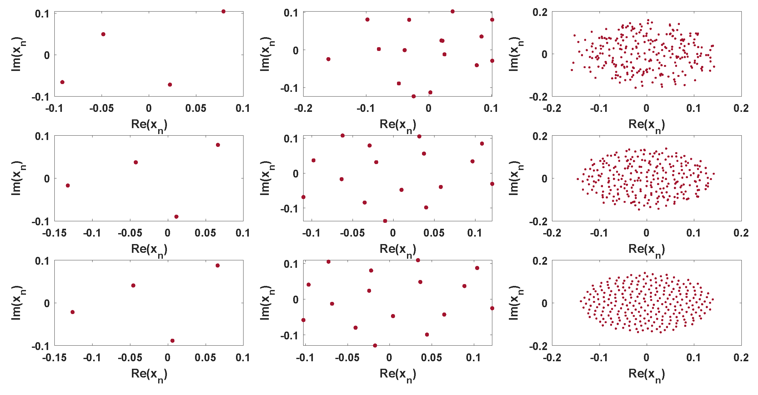
Figure 3.
Signal constellation of normalized Geometric Bell GAM with .
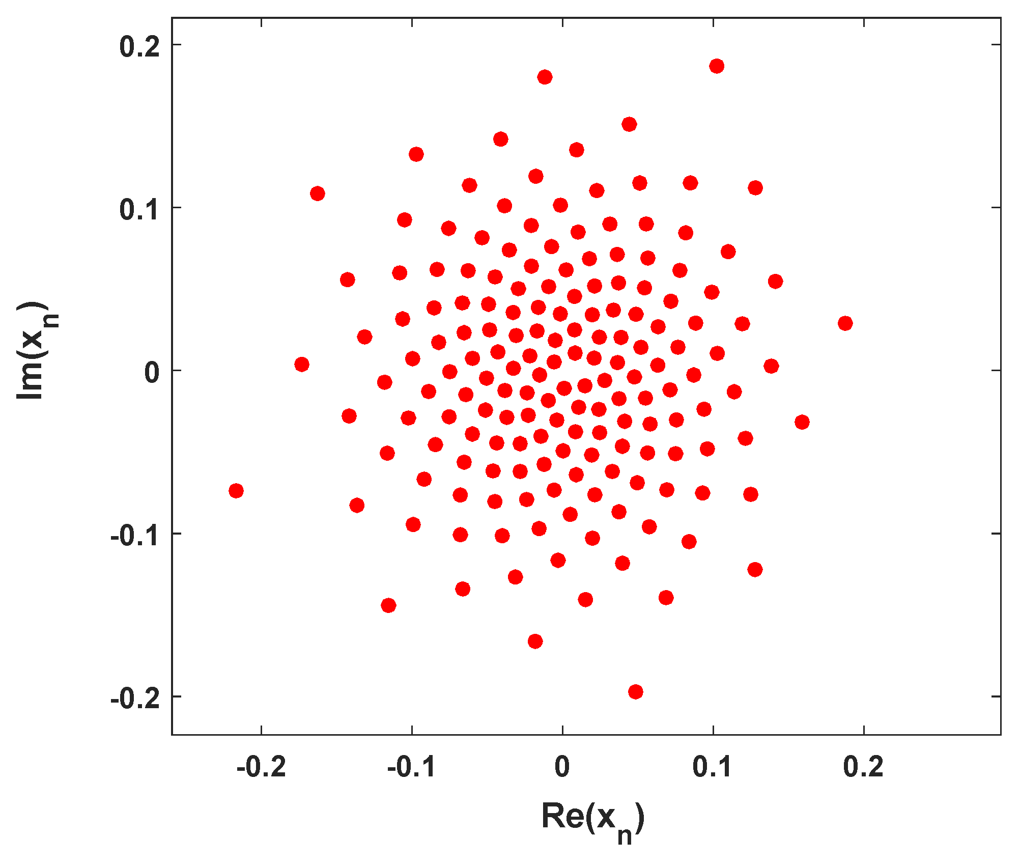
Figure 4.
The Upper/Lower bound for choosing the sum of series .
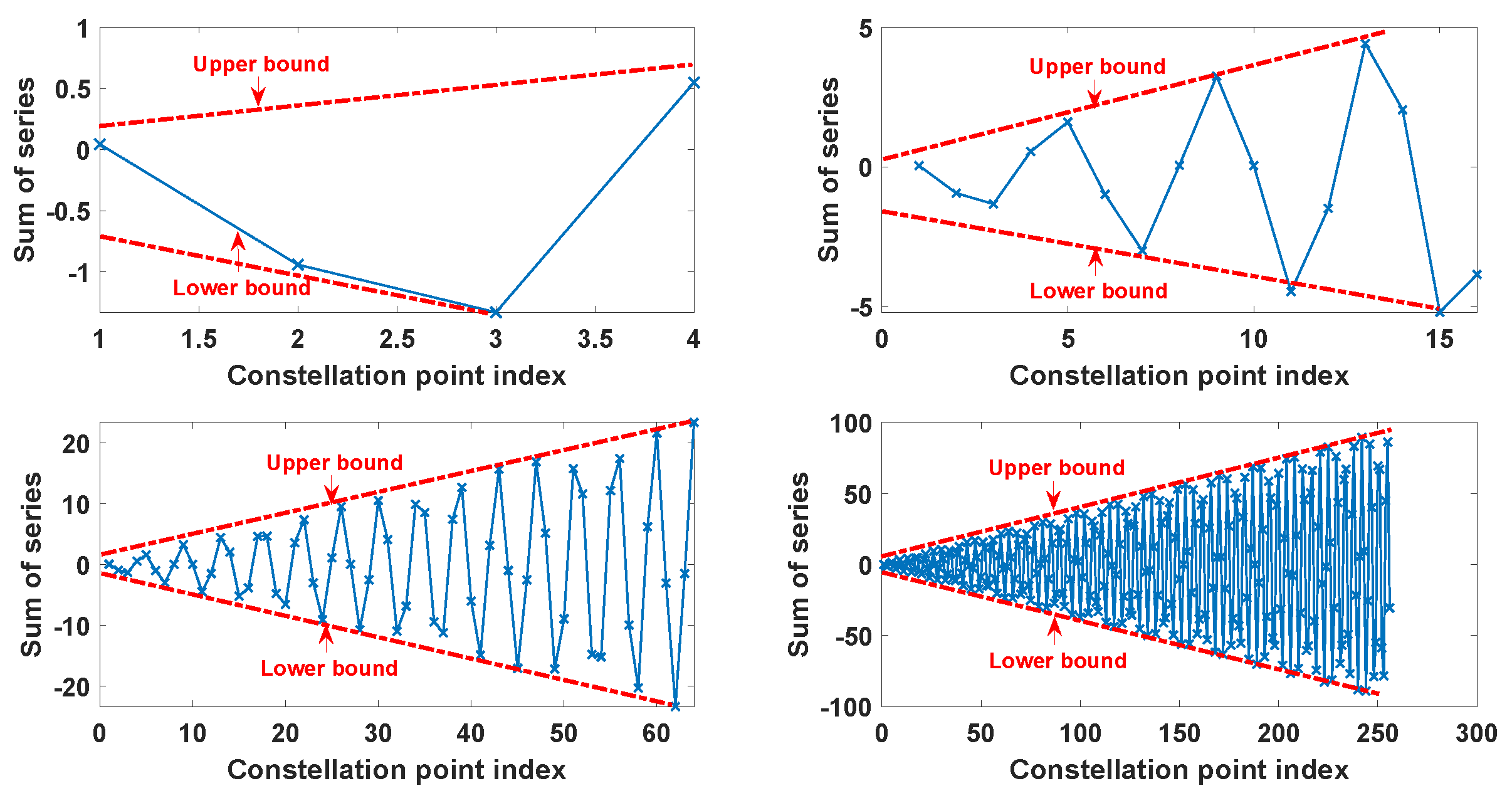
Figure 5.
Normalized Bd-GAM1 signal constellation with .
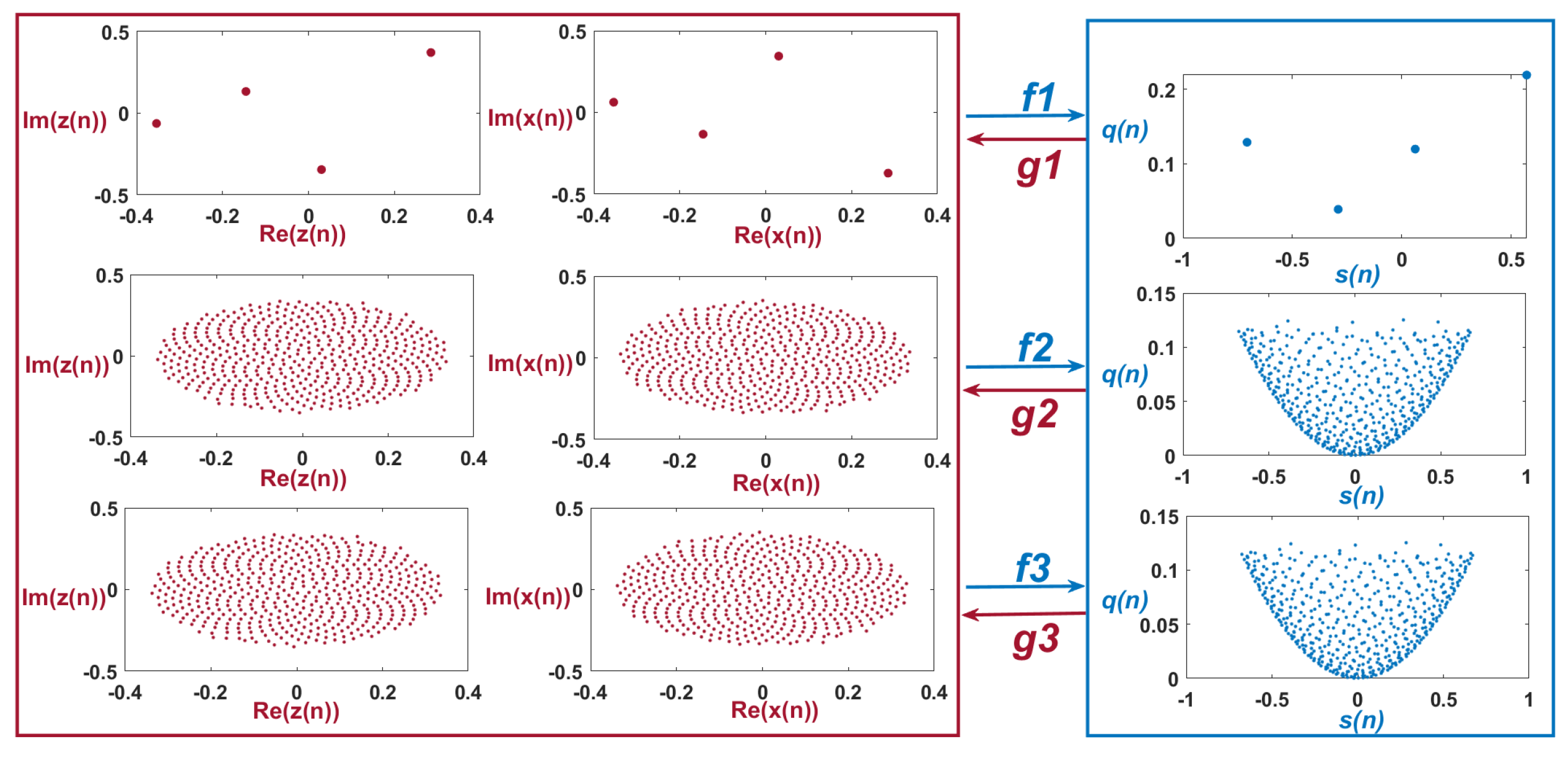
Figure 6.
Normalized Bd-GAM2 signal constellation with .
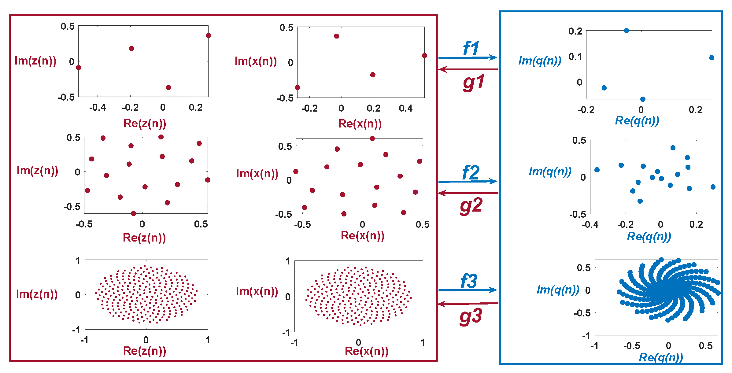
Figure 7.
Bd-GAM1/2 signal constellation aggregation.
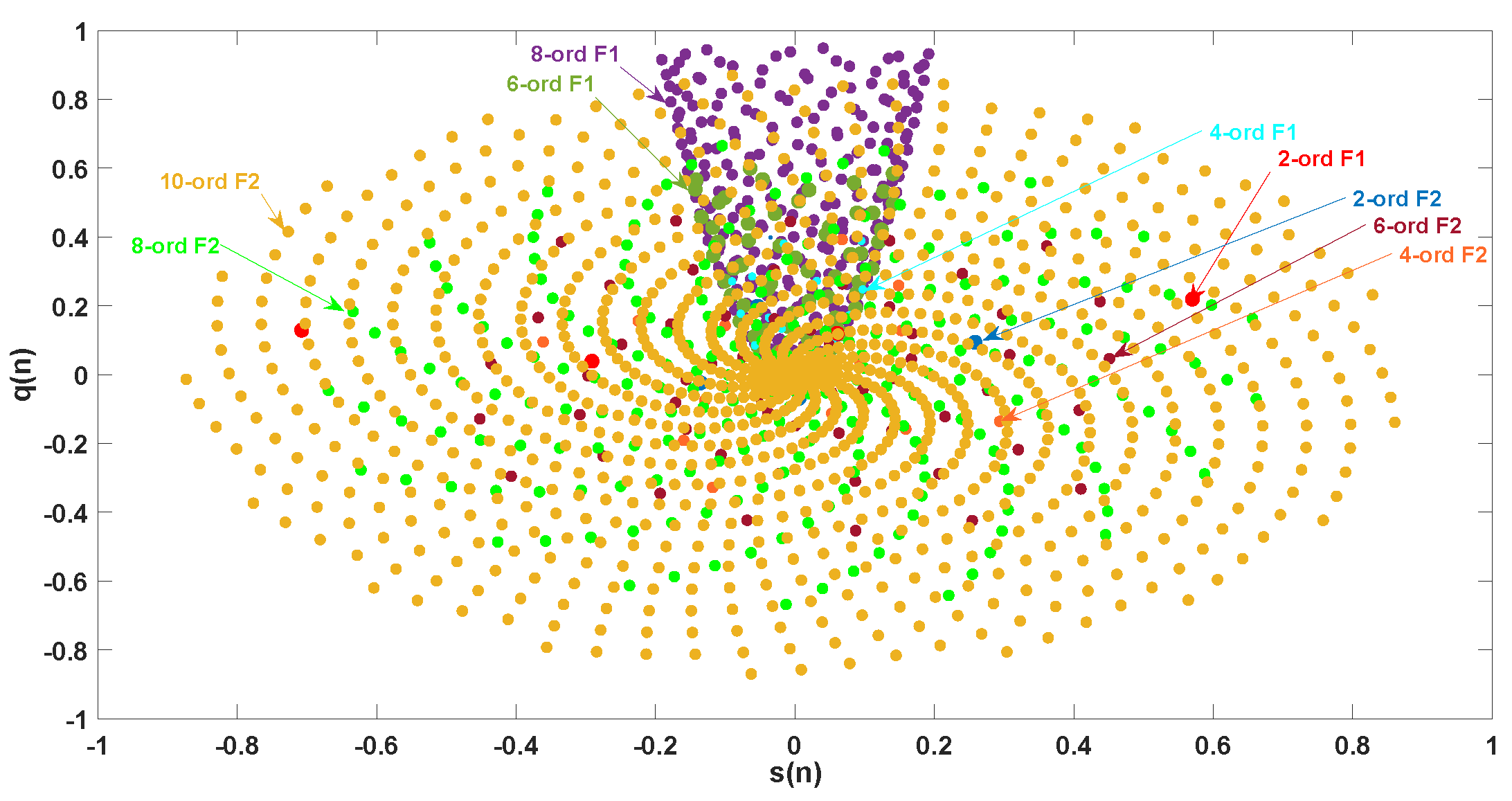
Figure 8.
Orbit for the points of Bd-GAM1/2.
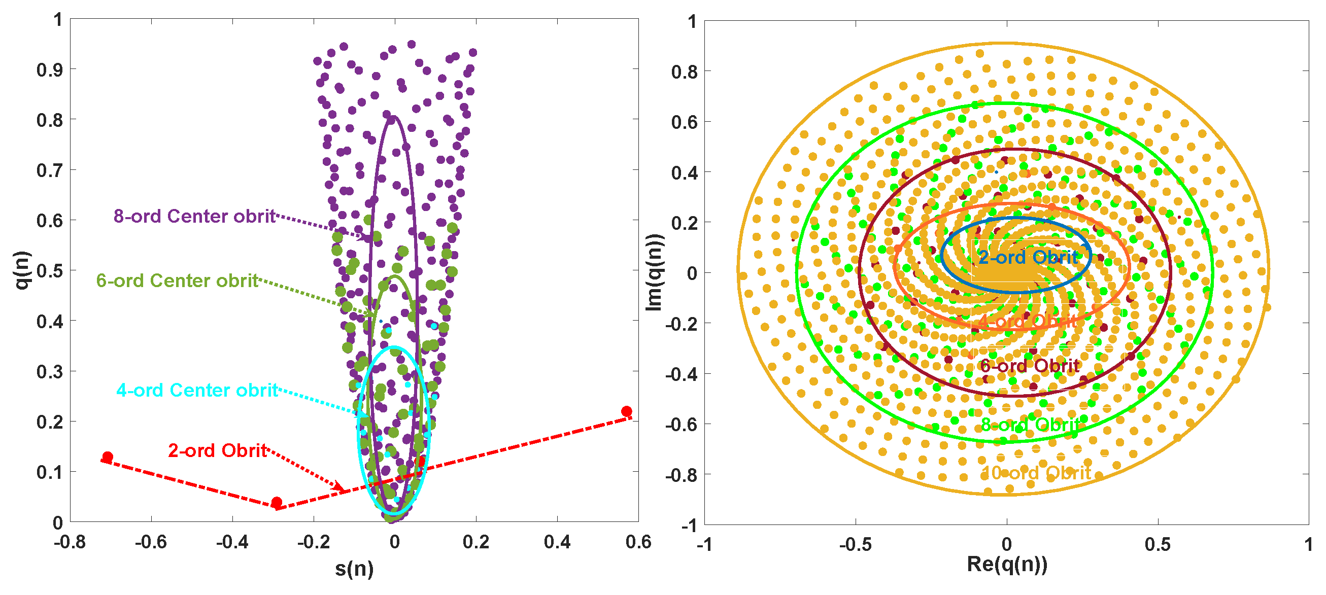
Figure 9.
Magnitude distribution of Bd-GAM1 with different constellation points ().
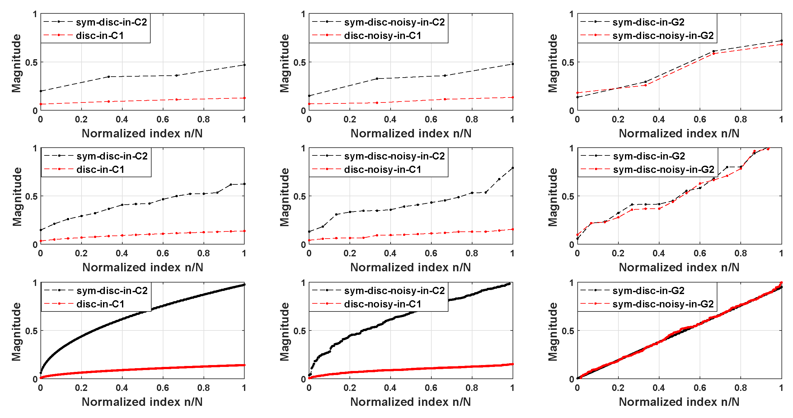
Figure 10.
Distance-performance for the Bd-GAM2.
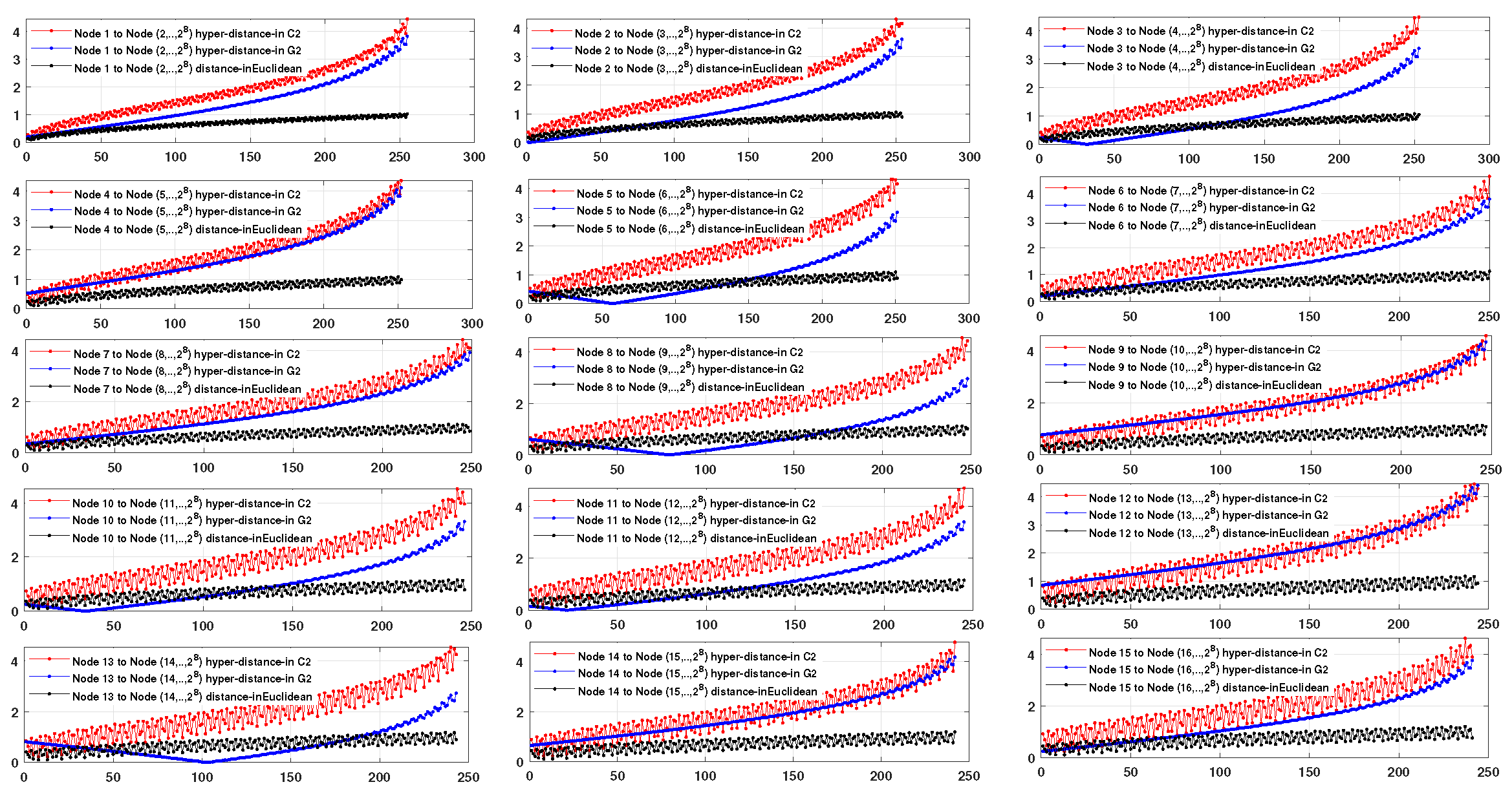
Figure 11.
MI of Bd-GAM1 with .
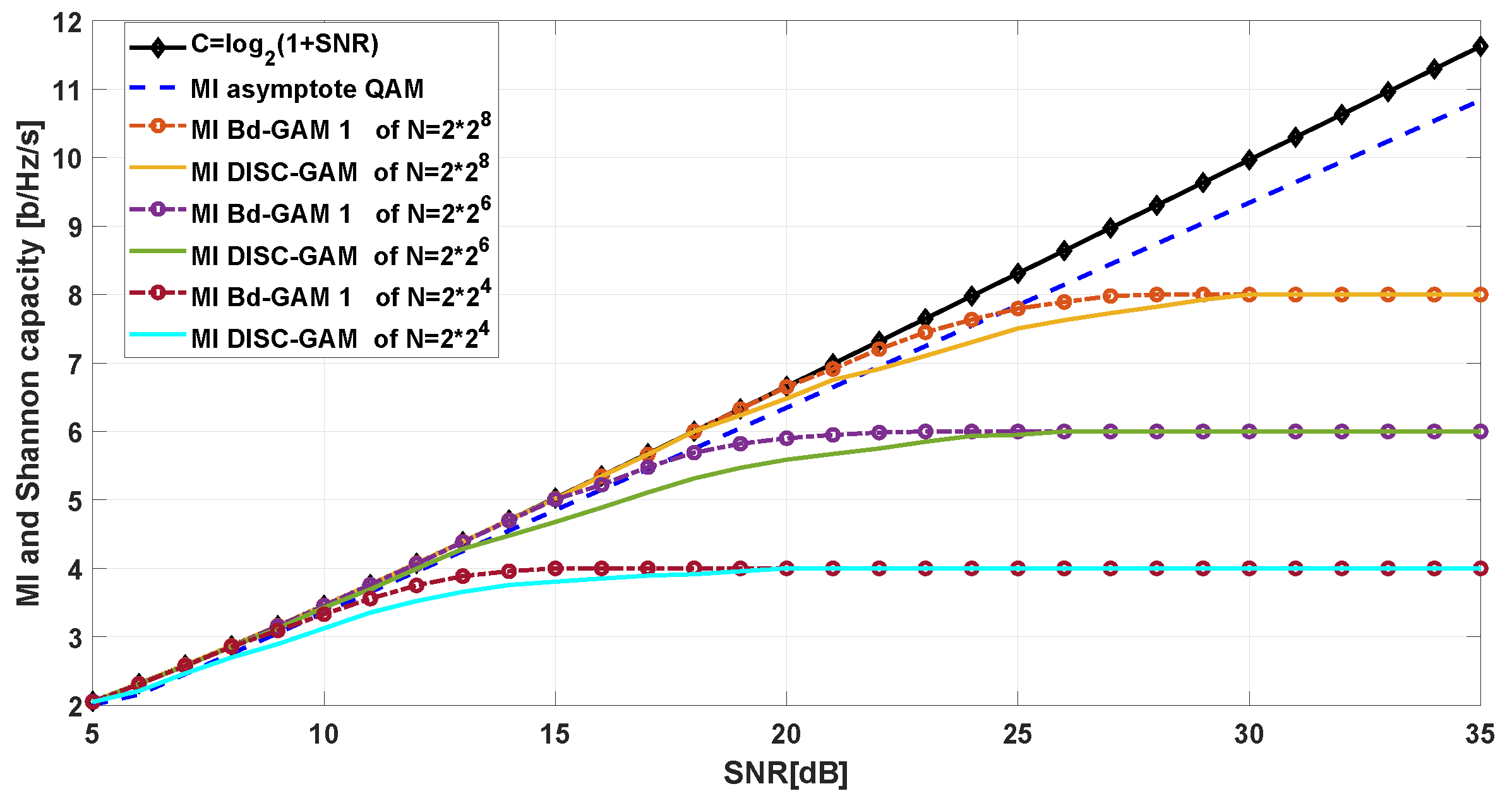
Figure 12.
MI of Bd-GAM2 with .
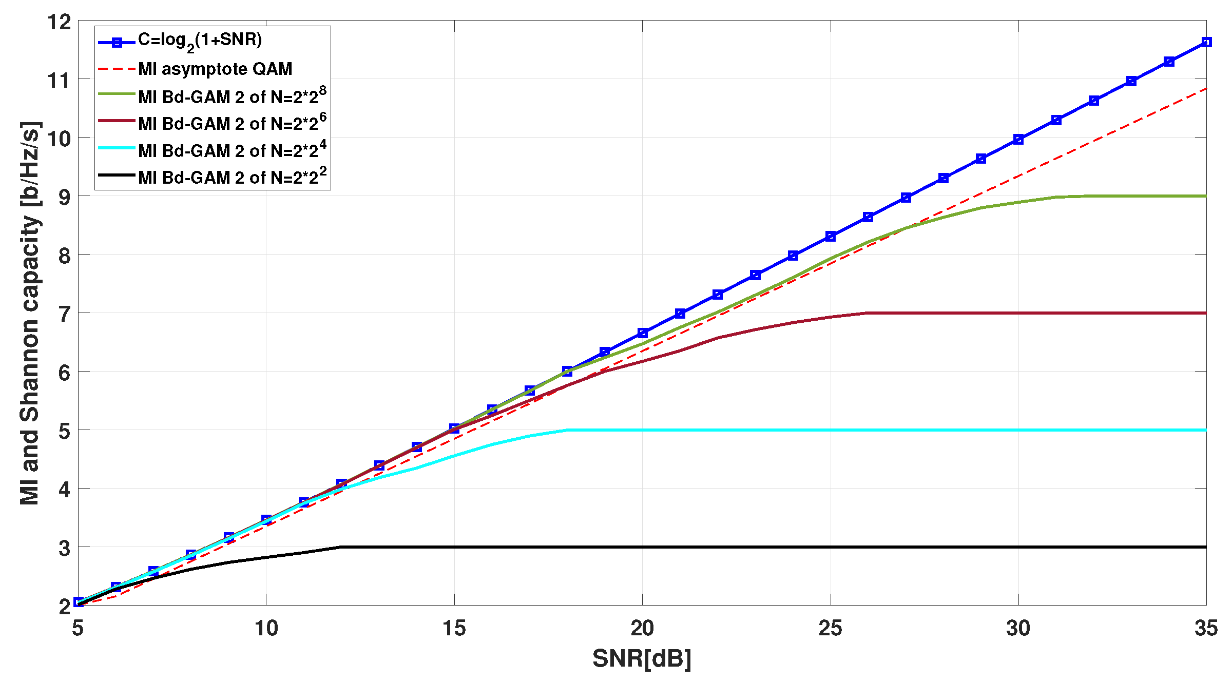

Table 1.
Entropy and PAPR values for different modulation methods 1.
| Modulation format | Entropy | PAPR () |
|---|---|---|
| Bd-GAM1 prop. | PAPR dB ≃ 1 dB | |
| Bd-GAM2 prop. | = | |
| Disc-GAM [12] | PAPR dB | |
| Geometric-bell-GAM [12] | PAPR | |
| Generalized Disc-GAM [14] | PAPR 2 dB |
1 As , the average power and peak power of QAM is higher than Disc-GAM with same average constellation point distances.
Disclaimer/Publisher’s Note: The statements, opinions and data contained in all publications are solely those of the individual author(s) and contributor(s) and not of MDPI and/or the editor(s). MDPI and/or the editor(s) disclaim responsibility for any injury to people or property resulting from any ideas, methods, instructions or products referred to in the content. |
© 2024 by the authors. Licensee MDPI, Basel, Switzerland. This article is an open access article distributed under the terms and conditions of the Creative Commons Attribution (CC BY) license (http://creativecommons.org/licenses/by/4.0/).
Copyright: This open access article is published under a Creative Commons CC BY 4.0 license, which permit the free download, distribution, and reuse, provided that the author and preprint are cited in any reuse.


