
Submitted:
20 December 2024
Posted:
23 December 2024
You are already at the latest version
Abstract
Mining activities generate substantial amounts of waste rock, which are often disposed of in waste rock piles. Drainage from these piles can pose serious environmental risks. It is crucial to reliably predict drainage properties in order to effectively manage them. In previous work, we developed a machine learning model to predict waste rock drainage quantity using weather monitoring data as input and drainage flow rate as output. However, this model lacked physical constraints, limiting its interpretability, reliability, and applicability. In this study, we introduced a new machine learning model designed with physical constraints to improve predictions of drainage quantity. This new model incorporates a weather refining sub-model and integrates physical constraints to enhance the overall reliability of the model predictions. The weather refining sub-model transforms primary weather features (total precipitation and temperature) into secondary features (rainfall, snowmelt, and evaporation) through established mathematical relationships. These secondary features were then used as inputs for the machine learning model to predict drainage quantity. To embed physical principles within the machine learning model, we integrated a water balance equation into the neural network architecture and modified the loss function accordingly. In addition, we included an adjustable bias term to optimize the balance between model performance and interpretability. Compared with our previous model, the incorporation of physical constraints into the machine learning model improved the accuracy of drainage quantity predictions. More importantly, this approach ensures that the model outputs adhere to physical laws, thereby enhancing its interpretability, reliability, and applicability.
Keywords:
drainage flow model
; hybrid machine learning
; water balance
; loss function modifications
1. Introduction
Large amounts of waste rock with diverse sizes and compositions are generated by mining activities and disposed in waste rock piles. The drainage from these piles, which often contain acid, elevated concentrations of sulfate and heavy metal(loid)s, can pose serious environmental risks and must be properly managed. Understanding the hydrology of waste rock piles is a crucial component of effective mine waste management [1]. Numerous studies have been conducted to characterize the hydrologic properties of these piles [2,3,4,5]. The highly heterogeneous nature of waste rock piles results in the formation of vastly different flow paths, causing infiltration rate to vary significantly, ranging from a few hours for preferential flow to several years for matrix flow to fully penetrate a waste rock pile [5,6,7,8]. Consequently, drainage flow is influenced not only by the present surface infiltration rate but also by those from previous periods.
Significant efforts have been made to develop models for predicting drainage quantity, which can generally be classified into three categories. The first category includes basic water balance models that correlate drainage quantity with precipitation and surface infiltration/run-off on a monthly or annual basis [9,10]. While useful, these models only provide rough estimates of drainage quantity based on weather monitoring data. The second category consists of models that incorporate fundamental principles, such as mass conservation, and constitutive equations, such as the Richards equation, to describe water movement in unsaturated porous media [10,11,12]. These models offer a more detailed and accurate prediction of the dynamic processes within waste rock piles [13,14]. Reactive transport models have also been developed to simulate drainage flow within heterogeneous waste rock piles [15,16,17,18,19]. However, it is often challenging for these models to fully capture the complex interactions among various factors influencing drainage flow, even though different methods such as probability density functions of physical and geochemical properties have been applied to simulate different degrees of heterogeneities [20,21]. In general, the application of these models requires comprehensive characterizations of each geologic unit within a waste rock pile to reliably predict drainage quantity. These characterizations can be prohibitively expensive or impossible to obtain.
Emerging machine learning models fall into the third category. Most of these models correlate drainage hydrological properties with directly monitored weather characteristics, such as temperature and precipitation [22,23,24]. Given that the relationship between weather characteristics and drainage quantity is often complex, these models typically use deep learning algorithms. However, training these models requires a large volume of data, which is often unavailable, to ensure that these models do not violate certain physical phenomena. To reduce the amount of data required for training, prior knowledge based on first principles has to be introduced into a model to improve the performance of the learning algorithms [25]. A common method for introducing physics into neural networks is by adding regularization terms derived from partial differential equations into the loss function [26]. However, the use of partial differential equations requires characterization data that are often difficult to obtain in the field, which can undermine the effectiveness of these physics-informed neural networks. For example, when introducing the Richards equation into neural networks, data required on soil water retention curves and unsaturated hydraulic conductivities are typically difficult to access, especially for waste rock piles with a high degree of heterogeneity.
In this research, we developed a machine learning model with physical constraints to predict drainage quantity. We applied a weather refining sub-model to first transform the directly monitored primary weather features into secondary ones, which were then used as inputs for the machine learning model. The novelty of this machine learning model lies in the integration of the water balance equation and the inclusion of physics-based constraints derived from partial derivatives within the loss function. This approach ensures that each term in the water balance equation adheres to fundamental physical laws. The model was then trained and tested with data from three monitoring stations.
2. Methodology
The methodology developed in this study for simulating drainage quantity consists of two sequential components: a non-machine learning weather refining sub-model and a machine learning drainage quantity model with physical constraints, as illustrated in Figure 1. The weather refining sub-model uses primary weather features, such as daily temperature and precipitation, as inputs. The primary weather features are directly measured by weather monitoring stations in the vicinity of waste rock piles. This sub-model transformed the primary weather features into secondary ones using established mathematical relationships. These secondary weather features were then used as inputs for the machine learning drainage quantity model (hereafter referred to as the “drainage quantity model”). The target (output) of the drainage quantity model is the drainage flow rate. Since drainage quantity is directly influenced by rainfall, snowmelt, and evaporation, transforming primary weather features to secondary features better reflects the underlying relationships between weather conditions and drainage. This transformation improves the physical interpretability of the model and simplifies the integration of physical constraints into the model. The weather monitoring stations and the waste rock piles from which drainage flow rate data were collected for model training are described in a previous article [24].
2.1. Weather Refining Sub-Model
The weather refining sub-model transforms primary weather features into secondary ones, which are then used as inputs for the drainage quantity model. To enhance data reliability, primary weather features from multiple weather monitoring stations near the waste rock piles were combined in the analysis. Missing value segments of varying lengths were addressed using appropriate interpolation methods to ensure a continuous dataset. After preprocessing, the data were used as inputs for the weather refining sub-model, which generated the secondary weather features through the following steps: (1) temperature adjustment; (2) precipitation differentiation; (3) snowmelt simulation; and (4) evaporation estimation.
Temperature adjustment: Although the weather monitoring stations are located near the waste rock piles, an elevation difference of 600 to 1000 m introduces potential discrepancies between the recorded weather data and the actual conditions on the piles. To address this, the lapse rate, which describes the rate of temperature decrease with increasing altitude, was used to adjust the recorded temperature data to reflect the actual ambient temperature on the piles [27].
Precipitation differentiation: The two forms of precipitation, rainfall and snowfall, have distinct impacts on water infiltration into waste rock piles, making it essential to differentiate between them. While weather stations provide precise precipitation data, elevation differences and resulting temperature variations can influence the actual form of precipitation on the waste rock piles. For this study, it was assumed that the total precipitation amount on the waste rock piles matched that recorded by the weather stations. However, the form of precipitation was determined based on the surface temperature, measured two meters above ground. Using the adjusted surface air temperature derived in the previous step, precipitation was classified as snowfall below a threshold surface temperature, which varies between 0 and 1.7 °C, and as rainfall above this threshold surface temperature [28]. The recategorized precipitation data provided a more accurate representation of rainfall and snowfall distributions on the waste rock piles.
Snowmelt simulation: Rainfall contributes directly to net infiltration into waste rock piles, whereas snowfall undergoes a more complex process involving accumulation and melting. To capture these processes, a snowmelt model was developed to transform past snowfall into daily snowmelt data. The model calculates the theoretical maximum daily snowmelt using Eq. 1, under the assumption of sufficient snow accumulation. The actual snowmelt for a given day is then determined as follows: if the snow cover for that day is not fully depleted, the actual snowmelt equals the theoretical maximum; if the snow cover for that day is depleted, the actual snowmelt equals the remaining snow from the previous day.
The degree-day factor method, adapted from LISFLOOD (a hydrological rainfall-runoff model), was applied to calculate the theoretical maximum daily snowmelt, as shown in Eq. 1 [29]. This model accounts for the contribution of rainfall to the snowmelt process.
In Eq. 1, M is the amount of snowmelt in mm, Cm (t) is the effective degree-day factor in mm/(℃‧day), which varies over time; R is the amount of rainfall (mm) during the time period Δt; Tair and Tmelt are the average air temperature (℃) and the snowmelt temperature over the time period Δt, respectively. Theoretically, Δt can be any time duration, and in this research, it was set to one day. The amount of snowmelt M was assumed to be zero when Tair ≤ Tmelt, meaning no snowmelt occurs if the air temperature is lower than or equal to the snowmelt threshold. Additionally, it is assumed that the degree-day factor Cm (t) follows a sinusoidal function with a period of one year. Its peak occurs at the summer solstice and its trough occurs at the winter solstice, reflecting seasonal variations in the snowmelt process.
Evaporation estimation: The daily evaporation rate in this research was estimated using a simplified version of the standard Penman equation proposed by [30]:
where E is the daily evaporation rate in mm/day; RS is the solar radiation reaching the ground surface; RA is the extraterrestrial solar radiation in MJ/(mm‧day); T is the daily mean temperature in
℃; RH is the relative humidity (%). If T + 9.5 ≤ 0, the daily evaporation rate E is considered zero. The solar radiation reaching the ground surface (RS) was estimated by downscaling observed historical solar radiation data using the ClimateNA software package [29]. The extraterrestrial solar radiation (RA) was calculated using theoretical formulas based on the Julian date and the latitude of the waste rock pile [30].
2.2. Machine Learning Drainage Quantity Model
2.2.1. Conceptual Model
The machine learning drainage quantity model developed in this research was built using TensorFlow version 2.3.0 in Python version 3.8.19. The model was developed based on the water balance principle for a waste rock pile, where the drainage quantity at any given time is determined by the contributions of rainfall, snowmelt, and evaporation. The schematic design of the model is illustrated in Figure 2. Before being used as inputs for the drainage quantity model, the secondary weather features– rainfall, snowmelt, and evaporation – generated by the weather refining sub-model were preprocessed using the rolling average method. This method calculates average values over varying time windows. Previous studies have shown that the use of this method smooths out high-frequency fluctuations and allows the model to use a broader range of measurements without increasing the number of time steps [23,24,31]. Additionally, waste rock volume was included as a feature due to its influence on water percolation through the waste rock pile.
Through their respective neural networks (NNRain, NNSnow, NNEvap, NNWRV, and NNBias), explained in detail in the following section, the inputs were transformed into effective contributions of rainfall (), snowmelt (), evaporation () to drainage quantity, and a bias term (). The drainage quantity was then calculated as the sum of effective contributions of rainfall and snowmelt, minus the effective contribution of evaporation, with the addition of the bias term.
2.2.2. Neural Network Architecture Design
As outlined in the previous section, NNRain, NNSnow, NNEvap, NNWRV, and NNBias represent the neural networks applied in the drainage quantity model. They were developed using five Gated Recurrent Units (GRUs), a type of modern recurrent neural networks [32]. GRUs were chosen due to their efficiency in handling time series data and their relatively swift architecture, making them well-suited for smaller datasets such as waste rock drainage data. Any of the neutral networks used could theoretically be replaced by other neural networks, such as long short-term memory (LSTM) cells or fully connected neural networks (FCNNs) with an extra flatten layer.
The inputs for the neutral networks were arranged as a three-dimensional tensor with the shape of (N, D, M), where N is the number of samples, D is the number of time steps, and M is the number of features. NNRain, NNSnow, and NNEvap are designed to use only their respective weather feature sequences as input, while NNWRV uses waste rock volume as its input (Eq. 3–6). The processes by which these neural networks transform inputs to outputs are represented as the following functions: , , , and . The outputs of these neutral networks are denoted as yrain, ysnow, yevap, and , respectively. It is important to note that yrain, ysnow, and yevap are scalar values, whereas is a three-dimensional vector. The components of serve as scale factors that adjust yrain, ysnow, and yevap to derive the effective contributions of rainfall (), snowmelt (), and evaporation () to drainage quantity, as shown in Eq. 7–9. These adjustments were specifically designed to account for the influence of waste rock volume on water percolation through the waste rock pile.
The NNbias, denoted by the function , was designed to predict the bias term (), as shown in Eq. 10. The inputs for NNBias include all weather features as well as the waste rock volume.
Eventually, the predicted mine waste rock drainage quantity () is calculated by Eq. 11:
To ensure meaningful physical interpretations, yrain, ysnow, yevap, and the three components of the vector should all be non-negative. To achieve this, LeakyReLU was chosen as the activation function for the output layers of NNRain, NNSnow, NNEvap and NNWRV. Although LeakyReLU may produce negative values, these values are typically very close to zero and can be treated as zero for water balance calculations. In contrast, the activation function for the output layer of NNBias was set to be linear, because the bias term can have both positive and negative values. This design ensures that each output is appropriately constrained in the model.
2.2.3. Loss Function Design
The loss function is a crucial component in machine learning, which quantifies the difference between the predicted outputs of a machine learning algorithm and the actual target values. In this study, apart from careful choice of activation functions as mentioned above, further physical constraints were embedded in the loss function to ensure that the correlations between the input and the output of the neural networks, NNRain, NNSnow, and NNEvap, are non-negative. The model training process involves minimizing the loss function by adjusting the internal parameters of the neutral networks represented by matrix θ. The optimal θ, denoted as θbest, is the value at which the loss function is minimized, as shown in Eq. 12.
where Loss represents the loss function, X represents the assembly of all inputs, and Q represents the OBSERVED drainage flow rate.
The loss function used in this study was designed to encompass three terms, defined as empirical loss, physical loss, and an extra regularization loss, as shown in Eq. 13:
The empirical loss was computed using the mean square error (MSE), which is the typical method of measuring the model performance in supervised machine learning. Specifically, this term measures the difference between the model predicted and the observed drainage flow rates, as shown in Eq. 14.
where is the batch size, and and are the observed and predicted drainage flow rate, respectively.
To enforce non-negative correlations between the output and the input of the neural networks, a physical constraint was incorporated into the model by introducing a physical loss term into the loss function. This term penalizes negative correlations by increasing its contribution to the loss in proportion to the magnitude of the negative correlation. The design of the physical loss term is shown in Eq. 15:
where , , and is the rainfall, snowmelt, and evaporation feature for sample i and time step j; The scale factor λp is a positive hyperparameter that ensures the physical loss value (Lphysical) comparable in magnitude to the empirical loss value (Lempirical). Like other hyperparameters, the value of λp needs to be fine-tuned. If λp is set too low, the penalty for negative correlations becomes negligible. Conversely, if λp is set too high, it can dominate the loss function, hindering the reduction of empirical loss during training and ultimately compromising the model performance.
Finally, an extra regularization loss term was introduced into the loss function to minimize the reliance of the model output on the bias term. The bias term () predicted by NNBias serves two purposes: firstly, it captures the interactions among weather features; secondly, it balances performance and interpretability of the model. The model training process aims to maximize the reliance of the model predictions on the effective contributions of the three weather futures and minimize the reliance on the bias term. The bias term only intervenes when the effective contributions of weather futures fail to satisfactorily predict the drainage quantity. This extra regularization loss term, shown in Eq. 16, was introduced to achieve this.
The scale factor λr is a positive hyperparameter controlling the contribution of the bias term to the model output. The contribution of the bias term can be manually adjusted or automatically adjusted by the model itself during the training process. A larger λr reduces the magnitude of the bias term, meaning that the model performance is sacrificed for a better model interpretability, and vice versa. During training, if the overall model performance is satisfactory, that is, the values of empirical loss (Lempirical) and physical loss (Lphysical) are relatively small, the optimizer of the model reduces the regularization loss (Lregularization) to achieve a smaller overall Loss, resulting in a smaller absolute value of the bias term. On the other hand, if the model performs poorly during training, the optimizer increases the Lregularization for a lower overall Loss, resulting in a higher absolute value of the bias term.
Furthermore, all five neutral networks were trained simultaneously, making them learn to collaborate during training. Besides predicting drainage quantity, the neural networks can also discern the contributions of various weather features to the drainage quantity.
2.2.4. Model Tuning
For the three drainage monitoring stations studied, the dataset available was divided into training and test set. Data from the last year of monitoring was chosen as the test set and the remaining data was used as the training set. The test set was completely isolated from the training and validation process. The training set was randomly and evenly divided into five folds for cross-validation to determine the best hyperparameter combination. Specifically, a Bayesian optimization algorithm was adopted to more efficiently search for the best combinations of hyperparameters [33]. Hyperparameters were searched simultaneously during cross-validation. The best combinations of hyperparameters for each drainage monitoring station are shown in Table 1. The Adam optimizer was chosen as the optimization algorithm for model training [34]. During model training, the batch size was fixed at four and did not participate in the model tuning process. A new model was built with the best hyperparameter combination and trained on all five folds to take full advantage of the monitoring data. Finally, the model was asked to give predictions on the test set for evaluation.
3. Results and Discussion
3.1. Model Training and Testing
Figure 3 compares the predicted and observed (measured) drainage flow rates during both model training and testing. The results indicate that the drainage quantity model generally fits the observed drainage flow rates well. However, the model fails to capture some peak flow events due to the lack of training data for such events. These peak flows, which typically last from a few hours to a day, posed a challenge for obtaining sufficient site measurement data for training the model. The trained model was successfully applied to predict the drainage flow rates using available weather monitoring data. The predicted drainage flow trend closely follows the historical measurements, suggesting that the model outputs are stable and reliable.
The performance of the drainage quantity model was quantitatively evaluated by two metrics: root mean square error (RMSE) and Nash–Sutcliffe efficiency (NSE), as shown in Table 2. The RMSE measures the average difference between predicted and observed drainage flow rates, with lower RMSE values indicating better model performance. Compared with our previously published model [24], the RMSE of the present model is reduced by 38% for Station 1, 44% for Station 2, and 9% for Station 3 in their respective test sets. However, RMSE alone cannot be used to compare model performance across stations, as it shares the same unit as the flow rate and varies with the average flow rate across stations. Therefore, the Nash–Sutcliffe efficiency (NSE) was also calculated to evaluate the model performance across different stations. A NSE value closer to 1 indicates better model performance. Based on the NSE values on the test sets, the model performed equally well at Station 1 and 2, and slightly worse on Station 3.
The bias term () was automatically adjusted during the training process to compensate for discrepancies between the predicted and the observed drainage flow rates. The monthly contributions of the bias term to the drainage quantity prediction are shown in Figure 4. On average, over the 12 months, the contribution of the bias term is 9% for Station 1, 31% for Station 2, and 18% for Station 3. The contributions of the bias term to the model output were considered acceptable, indicating that the drainage quantity predictions rely primarily on the effective contributions of the three weather features.
3.2. Sensitivity Tests
The trained model is designed to provide physically meaningful predictions, even when subjected to weather conditions that were previously unseen during training. To assess this, two sets of sensitivity tests were conducted on the test sets: one involving increasing the temperature (elevated temperature) and the other involving increasing the total precipitation (elevated precipitation). The model outputs of these two scenarios were compared with the original predictions for the three drainage monitoring stations. The results are shown in Figure 5.
When temperature is elevated, peak flow events occur earlier, which can be attributed to earlier onset of snowmelt. As a result of the early snowpack depletion and increased evaporation at higher temperatures, the predicted flow rates in summer are lower than those in the original predictions. For the elevated precipitation scenario, a greater amount of snow accumulates on top of the waste rock piles compared to the original estimation. As a result, the predicted flow rates are higher from June onward, due to a larger snowpack and slower depletion of the snowpack than the original predictions. The sensitivity test results demonstrate that the drainage model produces physically meaningful predictions when weather conditions are altered.
3.3. Verification of the Non-Negative Correlations by Monotonicity Test
After simultaneously training all five neural networks, NNRain, NNSnow, and NNEvap were isolated for monotonicity tests to verify that the physical loss term (Lphysical) described in Eq. 15 successfully enforced non-negative correlations between the inputs (rainfall, snowmelt, and evaporation) and the outputs (effective contributions of rainfall, snowmelt, and evaporation). To perform the monotonicity tests, the inputs for each neutral network were manually increased, and the corresponding predictions were evaluated against the original predictions. The monotonicity tests were conducted for two drainage quantity models: one was trained without the physical loss term, and the other was trained with it. The test without the physical loss term was achieved by setting λp to zero in Eq. 15. The results of the monotonicity tests are presented in Figure 6. The neural networks trained without the physical loss term exhibit some negative correlations, as some data points fall below the diagonal line, which is undesirable. In contrast, the neural networks trained with the physical loss term show a satisfactory non-negative monotonicity, with all data points positioned along or above the diagonal. The results highlight the importance of including the physical loss term in the loss function to maintain non-negative correlations.
3.4. The Impact of Current Weather Conditions on Future Drainage Quantities
The model developed in this study uses weather data up to the present day to predict the drainage quantity for the same day. It is practically valuable to evaluate how the accuracy of the model changes when using past and current weather data to predict future drainage quantities. To address this, the concept of ’lag days’ was introduced to represent the time difference (in days) between the most recent weather input data and the predicted drainage quantity. A new set of models was trained using the same methodology to make predictions and evaluations on datasets with varying lag days. The results are shown in Figure 7.
As expected, the performance of the model on the test set, as measured by NSE values, decreases as the number of lag days increases. However, the rate of performance deterioration varies across different stations. As the number of lag days increases, the performance of the model at Station 1 deteriorates the slowest, while the performance deteriorates the fastest at Station 2. At Station 3, the model performance declines gradually for the first three lag days, but then deteriorates more rapidly thereafter.
These tests enhanced our understanding of which aspects of the drainage flow rate are most influenced by recent rainfall and/or snowmelt events. For example, as shown in Figure 8, a peak flow observed at the end of June was accurately predicted by the original model with zero lag days. However, when the lag days were increased to three, the model completely missed this peak. This suggests that a rainfall or snowmelt event occurring within three days directly contributed to the peak flow, and the model with a three-day lag failed to predict it due to the absence of critical recent data.
4. Conclusions
This study introduces a machine learning model with embedded physical constraints to predict mine waste rock drainage quantities. Compared with our previously published model, the novelty of this model is that it incorporates physical constraints to ensure that the model outputs obey established physical laws. Weather monitoring data and drainage flow rate measurements from three monitoring stations were used for model training and testing.
The model comprises two main components: a weather refining sub-model and the machine learning drainage quantity model. First, the weather refining sub-model transforms primary weather features directly measured by monitoring stations–temperature and precipitation–to secondary ones, including rainfall, snowmelt, and evaporation. These transformations are based on well-established mathematical relationships. The machine learning model uses these secondary weather features and waste rock volume as inputs. Through their respective neural networks, these inputs were transformed to the effective contributions of rainfall, snowmelt, and evaporation to drainage quantity, with an extra bias term. The machine learning model incorporates physical constraints by embedding a water balance equation and including a physical loss term in the loss function. The water balance equation and the regularization loss term ensure that the drainage quantity is mainly determined by the effective contributions of rainfall, snowmelt, and evaporation. The physical loss term enforces the non-negative correlations between the inputs and outputs of the three neural networks associated with the weather features. Additionally, the inclusion of a bias term achieves balance between model performance and interpretability.
The model was successfully trained and validated using the provided datasets. Results from the monotonicity test confirmed that the inclusion of the physical loss term in the loss function successfully enforced non-negative correlations between the inputs and outputs of the three neural networks associated with the weather features. Sensitivity tests show that the model generates physically meaningful predictions, even under previously unseen weather conditions. The incorporation of physical constraints into the model enhances its interpretability, reliability, and applicability compared with our previously published model. The drainage quantity model developed in this study will be part of the subsequent development of a drainage quality model.
Funding
This research is financially supported by National Research Council Canada (NRC) Digital Health and Geospatial Analytics program (DHGA-117-1).
Data Availability Statement
In accordance with the policy, the code script for the model described in this paper cannot be open-sourced. However, we are committed to fostering academic collaboration and are willing to share the project codes for academic purposes. Interested parties are encouraged to contact the corresponding author for further details.
References
- Wolkersdorfer C, Nordstrom DK, Beckie RD, et al. Guidance for the Integrated Use of Hydrological, Geochemical, and Isotopic Tools in Mining Operations. Mine Water Environ. 2020, 39. [CrossRef]
- Tremblay GA, Hogan CM, eds. Mine Environment Neutral Drainage (MEND) Manual 5.4.2d: Prevention and Control. Canada Centre for Mineral and Energy Technology; 2001. http://mend-nedem.org/wp-content/uploads/5-4-2dVolume4_PreventionControlL.pdf.
- Lefebvre R, Hockley D, Smolensky J, Geélinas P. Multiphase Transfer Processes in Waste Rock Piles Producing Acid Mine Drainage; 1: Conceptual Model and System Characterization. J Contam Hydrol 2001;52(1-4). [CrossRef]
- Nichol CF. Transient Flow and Transport in Unsaturated Heterogeneous Media. Published online 2002.
- Nichol C, Smith L, Beckie R. Field-Scale Experiments of Unsaturated Flow and Solute Transport in a Heterogeneous Porous Medium. Water Resour Res. 2005, 41. [CrossRef]
- Brusseau ML, Rao PSC. Modeling Solute Transport in Structured Soils: a Review. Geoderma. 1990;46(1-3). [CrossRef]
- Flury M, Yates M V., Jury WA. Numerical Analysis of the Effect of the Lower Boundary Condition on Solute Transport in Lysimeters. Soil Sci Soc Am J. 1999, 63. [CrossRef]
- Smith L, López D, Beckie R. Hydrogeology of Waste Rock Dumps. Victoria, B.C. : British Columbia Ministry of Energy, Mines and Petroleum Resources and CANMET; 1995.
- Gélinas P, Lefebvre R, Choquette M. Monitoring of Acid Mine Drainage in a Waste Rock Dump. Miner Eng. 1992, 6, 212. [CrossRef]
- Gélinas P, Lefebvre R, Choquette M, Isabel D, Locat J, Guay R. Monitoring And Modeling of Acid Mine Drainage From Waste Rocks Dumps-La Mine Doyon Case Study. Canada Cent Miner Energy Technol. 1994;(June).
- Ramasamy M, Power C, Mkandawire M. Numerical Prediction of the Long-term Evolution of Acid Mine Drainage at a Waste Rock Pile Site Remediated with an HDPE-lined Cover System. J Contam Hydrol. 2018;216. [CrossRef]
- King, M. Groundwater and Contaminant Transport Modelling at the Sydney Tar Ponds. In: Proceedings of 56th Annual Canadian Geotechnical Conference and 4th Joint IAH-CNC/CGS Groundwater Specialty Conference. ; 2003, 10-26.
- Ma L, Huang C, Liu ZS, et al. A Full-Scale Case Study on the Leaching Process of Acid Rock Drainage in Waste Rock Piles and the Net Infiltration Through Cover Systems. Water Air Soil Pollut. 2020, 231. [CrossRef]
- Hendrickx JMH, Flury M. Uniform and Preferential Flow Mechanisms in the Vadose Zone. In: Conceptual Models of Flow and Transport in the Fractured Vadose Zone. ; 2001, 149-187.
- Pedretti D, Mayer KU, Beckie RD. Stochastic Multicomponent Reactive Transport Analysis of Low Quality Drainage Release from Waste Rock Piles: Controls of the Spatial Distribution of Acid Generating and Neutralizing Minerals. J Contam Hydrol. 2017;201. [CrossRef]
- Pedretti D, Beckie RD, Mayer KU. Risk Assessment of Acidic Drainage from Waste Rock Piles Using Stochastic Multicomponent Reactive Transport Modeling. Mine Water Circ Econ. Published online 2017, 696-702.
- Pedretti D, Vriens B, Skierszkan EK, Baják P, Mayer KU, Beckie RD. Evaluating Dual-Domain Models For Upscaling Multicomponent Reactive Transport in Mine Waste Rock. J Contam Hydrol. [CrossRef]
- Pedretti D, Mayer KU, Beckie RD. Controls of Uncertainty in Acid Rock Drainage Predictions from Waste Rock Piles Examined through Monte-Carlo Multicomponent Reactive Transport. Stoch Environ Res Risk Assess. [CrossRef]
- Liu ZS, Huang C, Ma L, et al. The Characteristic Properties of Waste Rock Piles in Terms of Metal Leaching. J Contam Hydrol 2019;226(August):103540. [CrossRef]
- Ma L, Huang C, Liu ZS, Morin KA, Aziz M, Meints C. Prediction of Acid Rock Drainage in Waste Rock Piles Part 2: Water Flow Patterns and Leaching Process. J Contam Hydrol 2021;242. [CrossRef]
- Smith L, Beckie R. Hydrologic and Geochemical Transport Processes in Mine Waste Rock. In: Environmental Aspects of Mine Wastes. Vol 31. ; 2003.
- Jiang C, Zhu S, Hu H, et al. Deep Learning Model Based on Big Data for Water Source Discrimination in an Underground Multiaquifer Coal Mine. Bull Eng Geol Environ. 2022, 81. [Google Scholar] [CrossRef]
- Ma L, Huang C, Liu ZS, Morin KA, Aziz M, Meints C. Artificial Neural Network for Prediction of Full-scale Seepage Flow Rate at the Equity Silver Mine. Water Air Soil Pollut . 2020, 231. [CrossRef]
- Zhang C, Ma L, Liu W. A Machine Learning Approach for Prediction of the Quantity of Mine Waste Rock Drainage in Areas with Spring Freshet. Minerals. 2023, 13. [Google Scholar] [CrossRef]
- Karniadakis GE, Kevrekidis IG, Lu L, Perdikaris P, Wang S, Yang L. Physics-Informed Machine Learning. Nat Rev Phys. 2021, 3, 422–440. [Google Scholar] [CrossRef]
- Tartakovsky AM, Marrero CO, Perdikaris P, Tartakovsky GD, Barajas-Solano D. Physics-Informed Deep Neural Networks for Learning Parameters and Constitutive Relationships in Subsurface Flow Problems. Water Resour Res 2020, 56. [CrossRef]
- Huschke, RE. Glossary of Meteorology. Vol 13.; 1960. [CrossRef]
- Laramie RL, Schaake JC. Simulation of the Continuous Snowmelt Process. Cambridge Ralph M. Parsons Laboratory for Water Resources and Hydrodynamics, Massachusetts Institute of Technology; 1972.
- Wang T, Hamann A, Spittlehouse D, Carroll C. Locally Downscaled and Spatially Customizable Climate Data for Historical and Future Periods for North America. PLoS One. 2016, 11. [CrossRef]
- Allen RG, Pereira LS, Raes D, Smith M. Crop Evapotranspiration - Guidelines for Computing Crop Water Requirements - FAO Irrigation and Drainage Paper 56.; 1998. [CrossRef]
- Ma L, Huang C, Liu ZS, Morin KA, Aziz M, Meints C. The Correlation between Drainage Chemistry and Weather for Full-Scale Waste Rock Piles Based on Artificial Neural Network. J Contam Hydrol. 2021;239(August 2020):103793. [CrossRef]
- Cho K, van Merriënboer B, Bahdanau D, Bengio Y. On the Properties of Neural Machine Translation: Encoder–decoder Approaches. In: Proceedings of SSST 2014 - 8th Workshop on Syntax, Semantics and Structure in Statistical Translation. ; 2014. [CrossRef]
- Bergstra J, Yamins D, Cox DD. Making a Science of Model Search: Hyperparameter Optimization in Hundreds of Dimensions for Vision Architectures. In: 30th International Conference on Machine Learning, ICML 2013. ; 2013.
- Kingma DP, Ba JL. Adam: A Method for Stochastic Optimization. In: 3rd International Conference on Learning Representations, ICLR 2015 - Conference Track Proceedings. ; 2015.
Figure 1.
A schematic of methodology developed in the present study for simulating waste rock drainage quantity.
Figure 1.
A schematic of methodology developed in the present study for simulating waste rock drainage quantity.
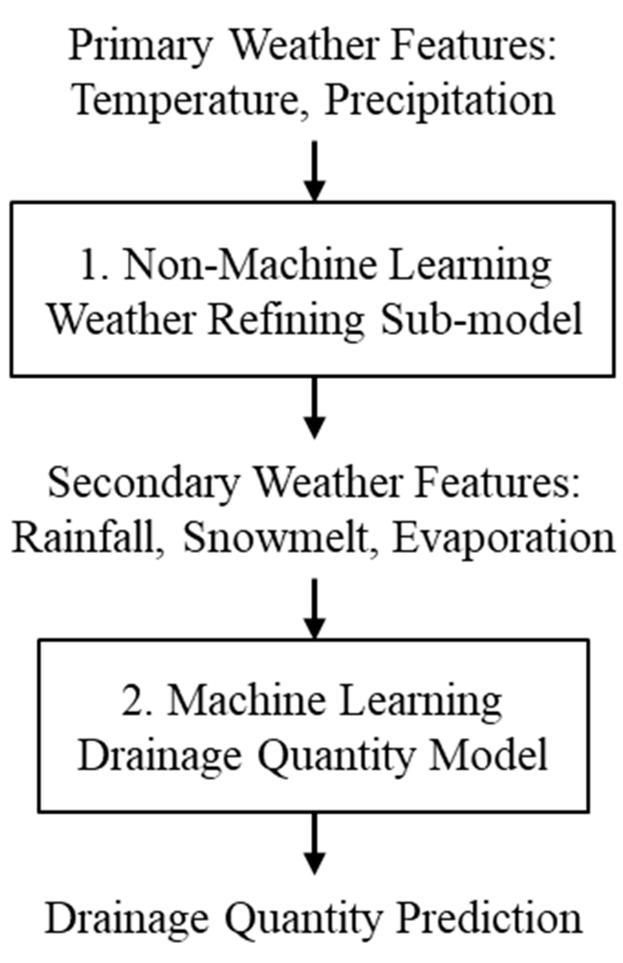
Figure 2.
A schematic of the neural network structure design for the drainage quantity model.
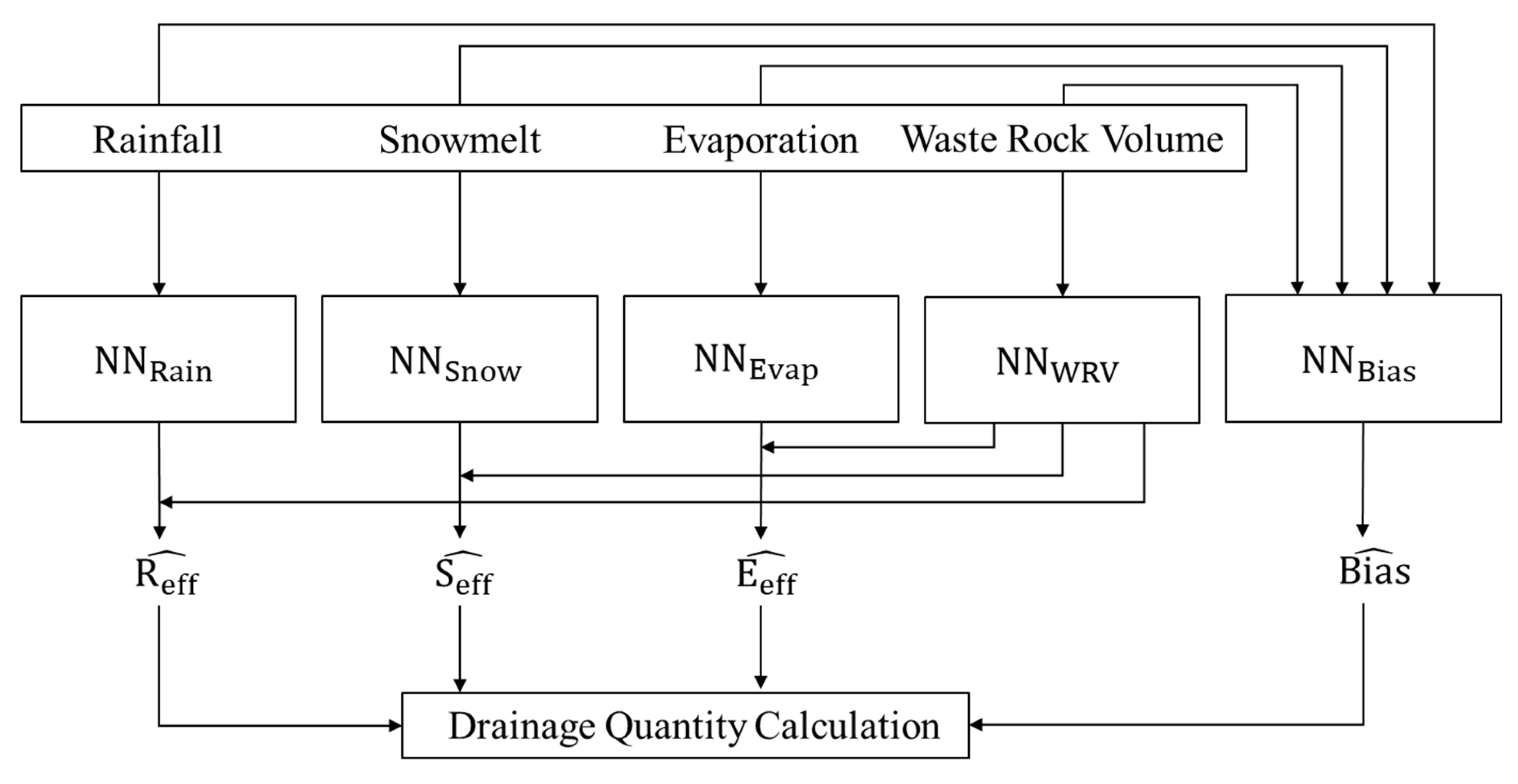
Figure 3.
Comparison of model output and measured drainage flow rate during model training and testing for the three drainage monitoring stations studied.
Figure 3.
Comparison of model output and measured drainage flow rate during model training and testing for the three drainage monitoring stations studied.
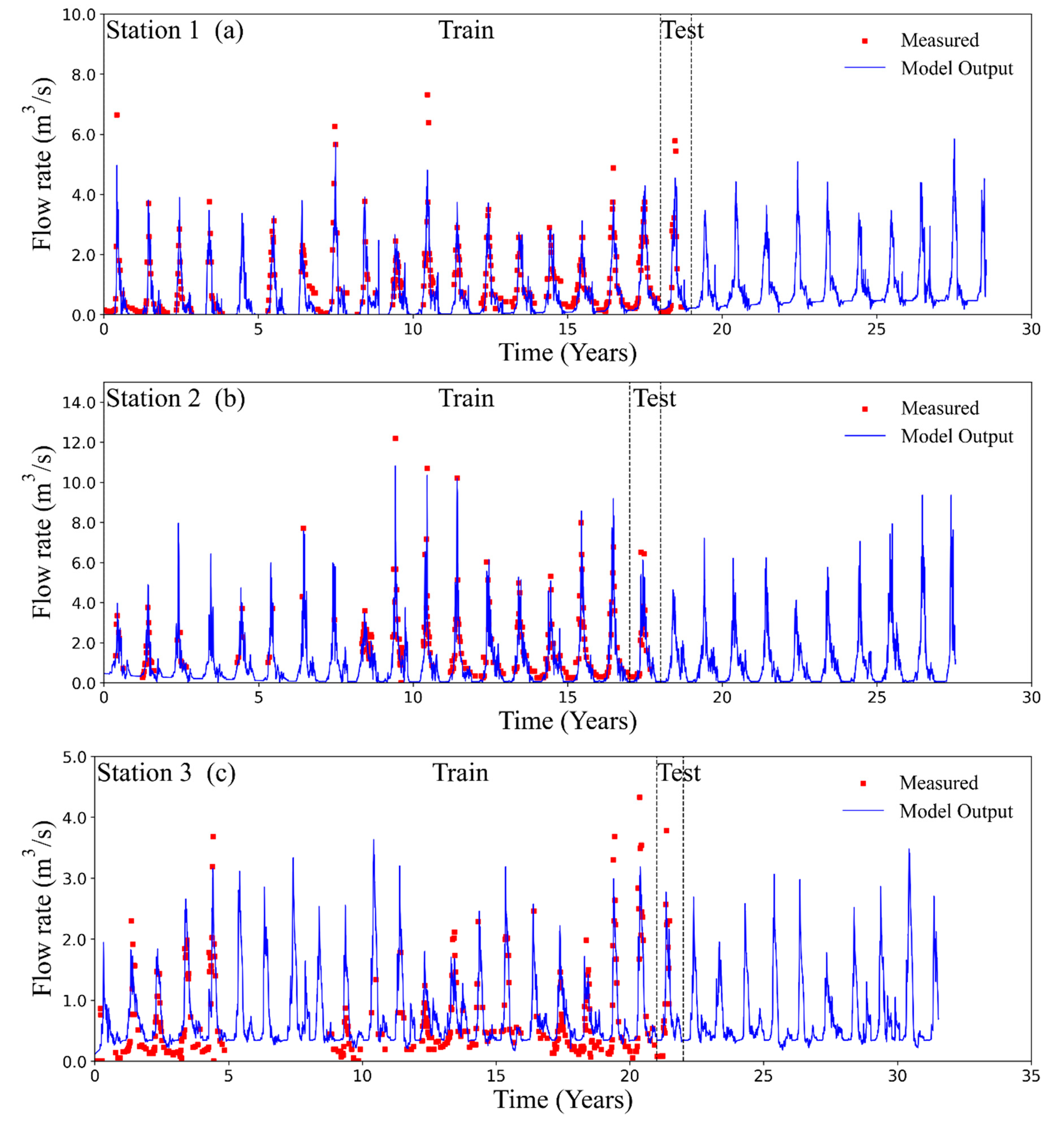
Figure 4.
The monthly contribution of the bias term to the drainage quantity prediction for the three drainage monitoring stations studied.
Figure 4.
The monthly contribution of the bias term to the drainage quantity prediction for the three drainage monitoring stations studied.
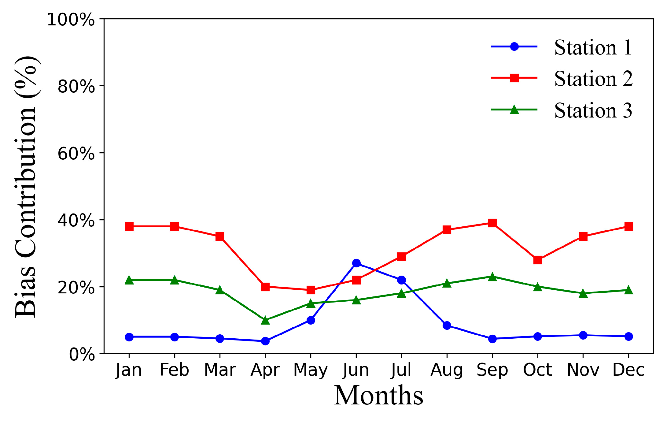
Figure 5.
Comparison of the sensitivity test results (one involving increasing temperature and the other involving increasing total precipitation) with the original predictions on the test sets for the three drainage monitoring stations.
Figure 5.
Comparison of the sensitivity test results (one involving increasing temperature and the other involving increasing total precipitation) with the original predictions on the test sets for the three drainage monitoring stations.
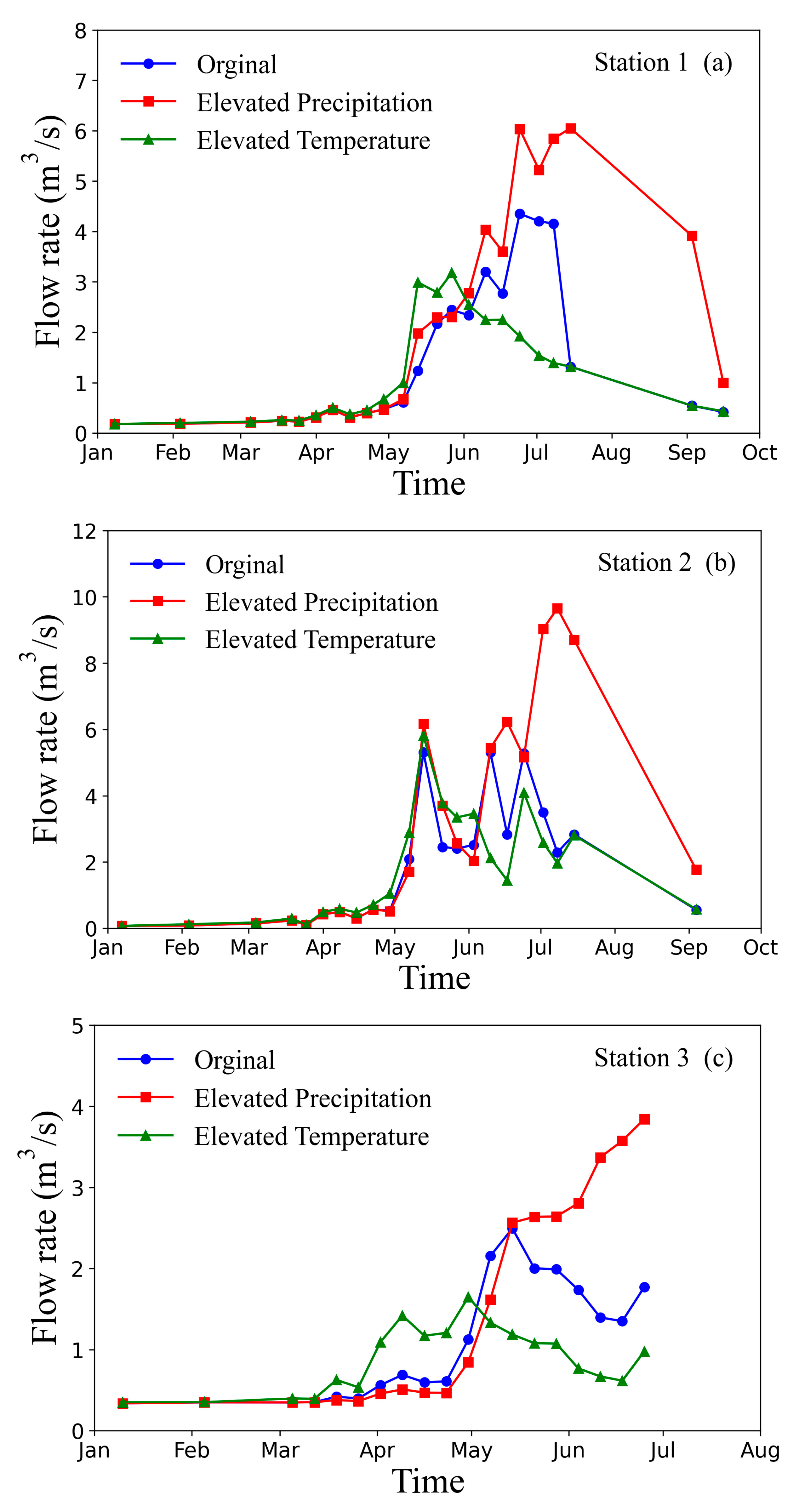
Figure 6.
Monotonicity test results for the drainage quantity model with and without the physical loss term in the loss function. Non-negative monotonicity means that all data points positioned along or above the diagonal.
Figure 6.
Monotonicity test results for the drainage quantity model with and without the physical loss term in the loss function. Non-negative monotonicity means that all data points positioned along or above the diagonal.
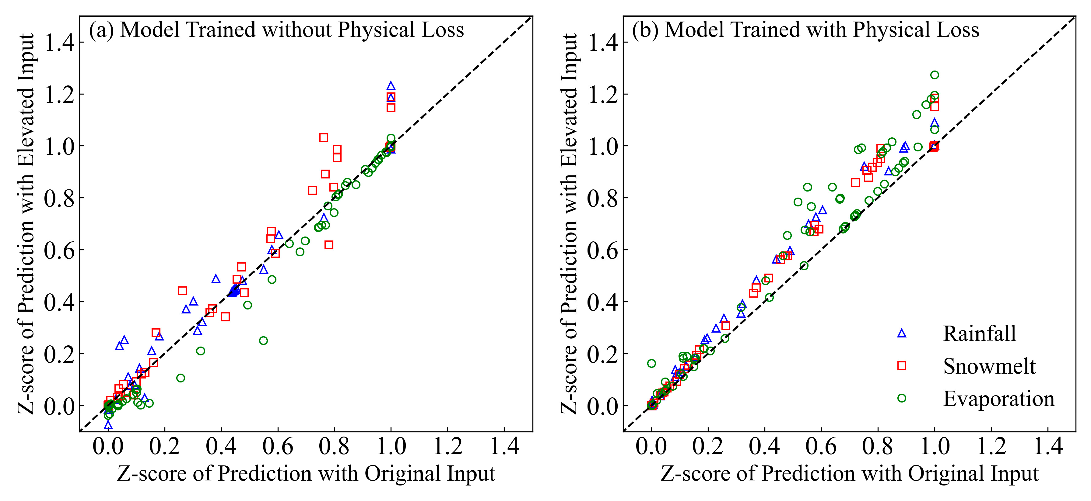
Figure 7.
The decrease of NSE scores on the test sets with increasing number of lag days for the three drainage monitoring stations.
Figure 7.
The decrease of NSE scores on the test sets with increasing number of lag days for the three drainage monitoring stations.
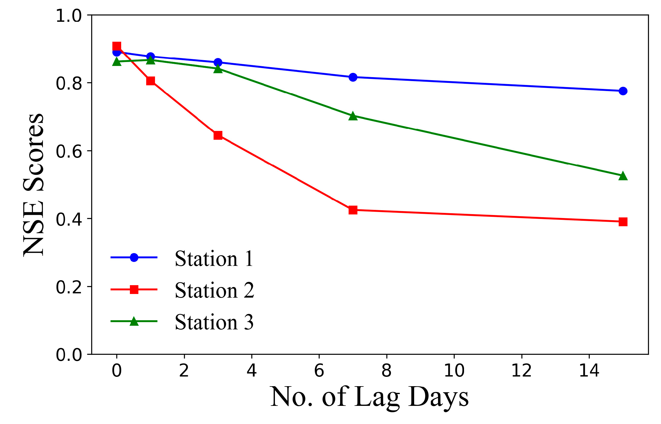
Figure 8.
Comparison of the drainage flow rates predicted by the original model, predicted by the model with three lag days, and the observed values on the test set of Station 1.
Figure 8.
Comparison of the drainage flow rates predicted by the original model, predicted by the model with three lag days, and the observed values on the test set of Station 1.
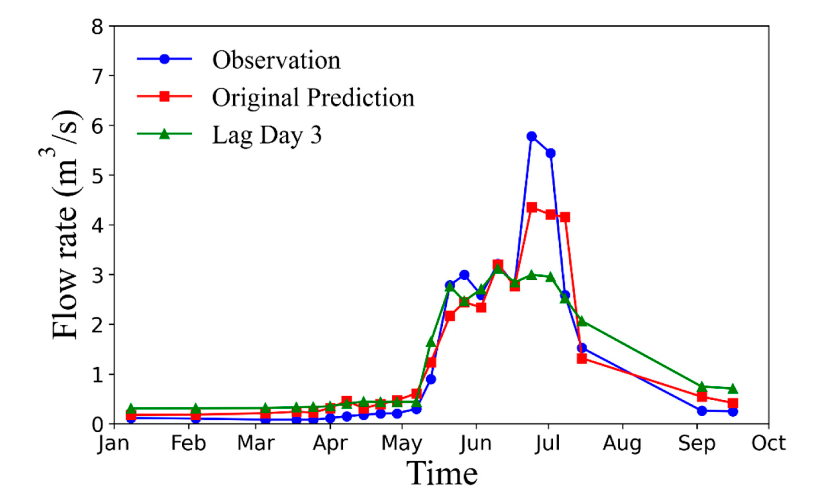

Table 1.
The best combination of hyperparameters for models trained for three waste rock drainage stations. Units are the dimensionality of the output space from the recurrent GRU layer; λp and λr are two scale factors mentioned in Eq. 15 and Eq. 16.
Table 1.
The best combination of hyperparameters for models trained for three waste rock drainage stations. Units are the dimensionality of the output space from the recurrent GRU layer; λp and λr are two scale factors mentioned in Eq. 15 and Eq. 16.
| Units | Learning rate | λp | λr | |
|---|---|---|---|---|
| Station 1 | 14 | 0.0005 | 1.5 | 1 |
| Station 2 | 32 | 0.0005 | 1.5 | 0.1 |
| Station 3 | 8 | 0.0005 | 1.5 | 0.1 |
Table 2.
The root mean square error (RMSE) and Nash–Sutcliffe efficiency (NSE) for evaluating the performance of the drainage quantity model during model training and testing.
Table 2.
The root mean square error (RMSE) and Nash–Sutcliffe efficiency (NSE) for evaluating the performance of the drainage quantity model during model training and testing.
| 1RMSE (m3/s) | RMSE (m3/s) | NSE | ||||
|---|---|---|---|---|---|---|
| Train | Test | Train | Test | Train | Test | |
| Station 1 | 0.4449 | 0.9175 | 0.5330 | 0.5701 | 0.8052 | 0.8904 |
| Station 2 | 0.9033 | 1.0108 | 0.4920 | 0.5660 | 0.9244 | 0.9082 |
| Station 3 | 0.2545 | 0.4400 | 0.4387 | 0.3985 | 0.8426 | 0.8616 |
1RMSE is for our previously published model, used as the benchmark.
Disclaimer/Publisher’s Note: The statements, opinions and data contained in all publications are solely those of the individual author(s) and contributor(s) and not of MDPI and/or the editor(s). MDPI and/or the editor(s) disclaim responsibility for any injury to people or property resulting from any ideas, methods, instructions or products referred to in the content. |
© 2024 by the authors. Licensee MDPI, Basel, Switzerland. This article is an open access article distributed under the terms and conditions of the Creative Commons Attribution (CC BY) license (http://creativecommons.org/licenses/by/4.0/).
Copyright: This open access article is published under a Creative Commons CC BY 4.0 license, which permit the free download, distribution, and reuse, provided that the author and preprint are cited in any reuse.


