The Generalized Characteristic Polynomial of the K_m,n-Complement of a Bipartite Graph

1. Introduction

In the present paper, we only consider undirected, simple, and connected graphs unless otherwise stated. Let $G=\left(V\right(G),E(G\left)\right)$ (or shortly $(V,E)$) be a graph with vertex set $V\left(G\right)$ and edge set $E\left(G\right)$. The adjacency matrix of G is defined as $A\left(G\right)=\left(a_{ij}\right)$, where $a_{ij}$ equals the number of edges connecting vertices $v_i$ and $v_j$ when $i\ne j$ and 0 when $i=j$. The rank of a graph G, denoted by $r\left(G\right)$, is defined to be the rank of its adjacency matrix $A\left(G\right)$. The degree matrix $D\left(G\right)$ is defined as the diagonal matrix $\mathrm{diag}(d_1,d_2,\dots ,d_n)$, where $n=\left|V\right|$, and $d_i$ equals the number of edges incident to vertex $v_i$. In the literature [1], Cvetković et al. introduced a bivariate polynomial, $\varphi (G;\lambda ,t)=det(\lambda I-(A\left(G\right)-tD\left(G\right)\left)\right)$ (abbreviated as $\varphi \left(G\right)$). Wang et al. [2] referred to it as the generalized characteristic polynomial of G. It is natural to define $A\left(G\right)-tD\left(G\right)$ in the variable t as the generalized matrix of a graph G, denoted by $M\left(G\right)={\left(m_{ij}\left(G\right)\right)}_{\left|V\right|\times \left|V\right|}$. To be specific,it is easy to see

$$m_{ij}\left(G\right)=\left\{\begin{array}{cc}-t{d}_G\left(v_i\right)\hfill & \mathrm{if}i=j,\hfill \\ 1\hfill & \mathrm{if}i\ne j\mathrm{and}{v}_i\sim v_j,\hfill \\ 0\hfill & \mathrm{otherwise}.\hfill \end{array}\right.$$

Consequently, the generalized characteristic polynomial of graph G is exactly the characteristic polynomial of the generalized matrix $M\left(G\right)$. That is, the polynomial $\varphi \left(G\right)=\varphi (G;\lambda ,t)=det(\lambda I-M(G\left)\right)=det(\lambda I-(A\left(G\right)-tD\left(G\right)\left)\right)$ is referred to as the generalized characteristic polynomial of G. Note that $A\left(G\right)-tD\left(G\right)$ with $t\in \mathbb{R}$ encodes several well-known graph matrices, such as the adjacency matrix, the Laplacian matrix, and the normalized Laplacian matrix. It is evident that the generalized characteristic polynomial of a graph generalizes several well-known polynomial invariants of graphs, for example:

• The characteristic polynomial of the adjacency matrix of a graph G is given by $\varphi (G;\lambda ,0)=det(\lambda I-A(G\left)\right)$;
• The characteristic polynomial of the Laplacian matrix $D\left(G\right)-A\left(G\right)$ of G is
  ${(-1)}^{\left|V\right|}\varphi (G;-\lambda ,1)=det(-\lambda I-A\left(G\right)+D\left(G\right))$;
• The characteristic polynomial of the unsigned Laplacian matrix $D\left(G\right)+A\left(G\right)$ of graph G is $\varphi (G;\lambda ,-1)=det(\lambda I-A(G)-D(G\left)\right)$;
• The characteristic polynomial of the normalized Laplacian matrix $I-D_G^{-{\displaystyle \frac{1}{2}}}{A}_G{D}_G^{-{\displaystyle \frac{1}{2}}}$ is ${(-1)}^{\left|V\right|}\varphi (G;0,-\lambda +1)=det(-A\left(G\right)-(\lambda -1)D\left(G\right))$.

Following [3], let $G=(V,E)$ be an undirected graph, if E is considered as a set of symmetric directed edges, meaning that if $e\in E$, then $\overline{e}\in E$, where $\overline{e}$ is the reverse edge of e, then G can also be viewed as a directed graph. For $e\in E$, let $h\left(e\right)$ denote the head of the directed edge e and $t\left(e\right)$ the tail of e. A closed walk in G is defined as a sequence of edges $C=(e_1,\dots ,e_k)$ such that $h\left(e_i\right)=t\left(e_{i+1}\right)$ for $i\in \mathbb{Z}/k\mathbb{Z}$. Here $k=\left|C\right|$ is the length of C and $cbc\left(C\right)=\#\{i\in \{1,\dots ,k\}\mid e_{i+1}=e_i\}$ is called the cyclic bump count of C. The notation $\left[C\right]$ is referred to as the equivalence class of the closed walk C under edge permutation, meaning that $(e_1,\dots ,e_k)\sim (e_2,\dots ,e_k,e_1)$. If none of the representatives of $\left[C\right]$ can be expressed as $C^k$ (for $k\ge 2$), then the cycle C is said to be irreducible. The set of all irreducible cycles is denoted by $\mathcal{C}$. The Bartholdi zeta function of a graph G is defined as (see [4] for details)

$$Z_G(\lambda ,t)=\prod _{\left[C\right]\in \mathcal{C}}{\displaystyle \frac{1}{1-{\lambda }^{cbc\left(C\right)}{t}^{\left|C\right|}}}.$$

The function $Z_G\left(t\right)=Z_G(0,t)$ is referred to as the (Ihara–Selberg) zeta function [5], which was introduced by Ihara to study the zeta function of a regular graph and its reciprocal, and the reciprocal of the zeta function of a regular graph was generalized to the reciprocal of the Bartholdi zeta function for a general graph G as below:

$$Z_G{(\lambda ,t)}^{-1}={\left(1-{(1-\lambda )}^2{t}^2\right)}^{\left|E\right|-\left|V\right|}det\left(I-t{A}_G+(1-\lambda )(D_G-(1-\lambda )I)t^2\right).$$

In particular, the reciprocal of the zeta function for a general graph G is given by:

$$Z_G{\left(t\right)}^{-1}={(1-t^2)}^{\left|E\right|-\left|V\right|}det\left(I-t{A}_G+t^2(D_G-I)\right).$$

The zeta function encodes significant structural information about the graph, such as the number of vertices, edges, and loops. Moreover, the number of spanning trees (the complexity of the graph) $\tau \left(G\right)$ satisfies the equation [6]:

$${\displaystyle \frac{\partial f_G\left(t\right)}{\partial t}}{|}_{t=1}=2\left(\right|E|-\left|V\right|)\tau \left(G\right),\mathrm{where}{f}_G\left(t\right)=det\left(I-t{A}_G+t^2(D_G-I)\right).$$

For a comprehensive treatment of many aspects of Zeta function, refer to [7].

Zeta functions of certain classes of graphs have received considerable attention, such as the line graph of semi-regular bipartite graphs [8], the middle graph of semi-regular bipartite graphs [9], the cone graph of regular graphs [10], and various special join graphs of regular graphs [11,12]. It is not difficult to prove that $\varphi (G;\lambda ,t)$ determines the reciprocal of the zeta function, and vice versa [13]. Let $G=(V,E)$ be a subgraph of the complete bipartite graph $K_{m,n}$. The $K_{m,n}$-complement of G is defined as the graph obtained from $K_{m,n}$ by deleting all edges of G in $K_{m,n}$, i.e., $K_{m,n}-E\left(G\right)$. In this paper, we shall show a computational method for deriving the formula for the generalized characteristic polynomial of the $K_{m,n}$-complement of any bipartite graph G, and further give an explicit formula for the generalized characteristic polynomials of the $K_{m,n}$-complement of a bipartite graph with rank less than or equal to 4.

2. Notations and Terminology

Let $G=(V,E)$ be a graph with the vertex set $V=\{v_1,v_2,\cdots ,v_n\}$ and the edge set $E=\{e_1,\cdots ,e_m\}$. For two vertices $v_i,v_j\in V$, if $v_i$ and $v_j$ are adjacent, we denote this as $v_i\sim v_j$. The neighborhood of a vertex $v_i$ in G is defined as $N_G\left(v_i\right)=\{v_j\in V\mid v_i\sim v_j\}$, and the degree of vertex $v_i$ in G is denoted by $d_i=d_G\left(v_i\right)=\left|N_G\left(v_i\right)\right|$. The complement of the graph $G=(V,E)$ is denoted as $G^c=(V,E^c)$, where $E^c=\{v_i{v}_j\mid v_i,v_j\in V,v_i{v}_j\notin E\}$. If $G=(V,E)$ and $G^{\prime }=(V^{\prime },E^{\prime })$ with $V^{\prime }\subseteq V$ and $E^{\prime }=\{(u,v)\mid u,v\in V^{\prime },(u,v)\in E\}$, then $G^{\prime }$ is referred to as an induced subgraph of G.

A graph $G=(V,E)$ is a bipartite graph if and only if there exists a bipartition of V into $(V_1,V_2)$ (namely $V=V_1\cup V_2,V_1\cap V_2=\varnothing$) such that no two vertices within $V_1$ or $V_2$ are adjacent. If the sizes of the bipartition sets are equal, i.e., $|V_1|=|V_2|$, then G is said to be a balanced bipartite. If $G=(V,E)$ is a bipartite graph with a bipartition $(V_1,V_2)$, the bipartite complement of G, denoted as $G^{bc}$, has vertex set $V\left(G^{bc}\right)=V\left(G\right)$ and edge set $E\left(G^{bc}\right)=\{xy\mid x\in V_1,y\in V_2,xy\notin E\left(G\right)\}$. For a bipartite graph G, its adjacency matrix is given by

$$A\left(G\right)=\left[\begin{array}{cc}0& B\left(G\right)\\ B^T\left(G\right)& 0\end{array}\right],$$

where $B\left(G\right)={\left(b_{ij}\right)}_{m\times n}$ is the bipartite adjacency matrix of G that defines the vertex adjacency relationship between the bipartite sets $V_1$ and $V_2$. Specifically,

$$b_{ij}=\left\{\begin{array}{cc}1\hfill & v_i\sim v_j,v_i\in V_1,v_j\in V_2\hfill \\ 0\hfill & \mathrm{otherwise}.\hfill \end{array}\right.$$

Lemma 1

([14]).

Let G be a balanced bipartite graph. If G has a unique perfect matching, then the bipartite adjacency matrix $B\left(G\right)$ has determinant 1 or $-1$.

Lemma 2

([15]).

Let $A={\left(a_{ij}\right)}_{n\times n}$ be an $n\times n$ matrix, and let D be a diagonal matrix with diagonal entries $d_1,d_2,\dots ,d_n$, i.e., $D=\mathrm{diag}(d_1,d_2,\dots ,d_n)$. Then

$$det(A+D)=\sum _{\theta \subseteq \left[n\right]}det\left(A_{\theta }\right)det\left(D_{\overline{\theta }}\right),$$

(1)

where θ is a subset of $\left[n\right]=\{1,2,\dots ,n\}$ and $\overline{\theta }$ is the complement of θ in $\left[n\right]$, namely $\overline{\theta }=\{k\mid k\in \left[n\right],k\notin \theta \}$; $A_{\theta }$ is the submatrix formed by the rows and columns of A indexed by θ. By convention, $det\left(A_{\varnothing }\right)=1$.

The following lemma immediately follows from Lemma 2.

Lemma 3

([15]). If D is an invertible matrix, then the determinant of the matrix $A+D$ can be expressed as

$$det(A+D)=det\left(D\right)\sum _{\theta \subseteq \left[n\right]}{\displaystyle \frac{det\left(A_{\theta }\right)}{det\left(D_{\theta }\right)}}.$$

(2)

Lemma 4

([16]). Let A be an $n\times n$ matrix. If there exists a $p\times q$ zero submatrix in A such that $p+q\ge n+1$, then $det\left(A\right)=0.$

3. The generalized characteristic polynomial

For the sake of simplicity, the complete graph, cycle, and path on n vertices are denoted by $K_n$, $C_n$, and $P_n$, respectively. Notationally, for $m,n\in \mathbb{Z}$, $\left[m\right]=\{1,2,\dots ,m\}$ and $[m+1,m+n]=\{m+1,m+2,\dots ,m+n\}$; $I_n$ and $J_{m\times n}$ (or $J_n$) respectively denote the $n\times n$ identity matrix and the $m\times n$ (or $n\times n$) matrix of all ones. For the rest of this paper, we will use $K_{m,n}$ to symbolize the complete bipartite graph with bipartite partition $(X,Y)$, where $X=\{v_1,v_2,\dots ,v_m\}$ and $Y=\{v_{m+1},v_{m+2},\dots ,v_{m+n}\}$, and ${\mathcal{B}}_{m,n}$ to symbolize the set of all bipartite graphs with bipartite partition $(X,Y)$ such that $\left|X\right|=m$ and $\left|Y\right|=n$. Note that a graph $G\in {\mathcal{B}}_{m,n}$ if and only if its bipartite complement $G^{bc}\in {\mathcal{B}}_{m,n}$. Let G be a subgraph of the complete bipartite graph $K_{m,n}$. The $K_{m,n}$-complement of a subgraph G in $K_{m,n}$ is defined as the graph obtained from $K_{m,n}$ by deleting all edges of G in $K_{m,n}$, denoted by $K_{m,n}-G$.

Theorem 1.

Let $G=(V,E)$ be a subgraph of $K_{m,n}$ with bipartite partition $(X,Y)$ mentioned previously, and G has a bipartite partition $(V_1,V_2)$ such that $V_1\subseteq X$ ($|V_1|=s$), $V_2\subseteq Y$ ($|V_2|=t$). Then, we have

$$\begin{array}{cc}\hfill & \varphi (K_{m,n}-G)\hfill \\ \hfill & ={(nt+\lambda )}^{m-s}{(mt+\lambda )}^{n-t}\prod _{v\in V_1}((n-d_G\left(v\right))t+\lambda )\prod _{v\in V_2}((m-d_G\left(v\right))t+\lambda )\hfill \\ \hfill & ·\left[1+\sum _{Q^{bc}\in \mathcal{G}\left(H^{bc}\right)}{\displaystyle \frac{{(-1)}^{\frac{\left|V\right(Q^{bc}\left)\right|}{2}}{\left(det(J_k-B\left(Q^{bc}\right))\right)}^2}{\prod _{v\in V\left(Q^{bc}\right)\cap X}((n-d_G\left(v\right))t+\lambda )\prod _{v\in V\left(Q^{bc}\right)\cap Y}((m-d_G\left(v\right))t+\lambda )}}\right]\hfill \\ \hfill & ={(nt+\lambda )}^{m-s}{(mt+\lambda )}^{n-t}\prod _{v\in V_1}((n-d_G\left(v\right))t+\lambda )\prod _{v\in V_2}((m-d_G\left(v\right))t+\lambda )\hfill \\ \hfill & ·\left[1+\sum _{Q\in \mathcal{G}(K_{m,n}-G)}{\displaystyle \frac{{(-1)}^{\frac{\left|V\right(Q\left)\right|}{2}}{\left(det\left(B\right(Q\left)\right)\right)}^2}{\prod _{v\in V\left(Q\right)\cap X}((n-d_G\left(v\right))t+\lambda )\prod _{v\in V\left(Q\right)\cap Y}((m-d_G\left(v\right))t+\lambda )}}\right],\hfill \end{array}$$

(3)

where $\mathcal{G}\left(H^{bc}\right)$ is the set of all induced balanced bipartite subgraphs $Q^{bc}$ in H such that the bipartite complement Q of $Q^{bc}$ has a nonsingular biadjacency matrix $B\left(Q\right)$; $\mathcal{G}\left(H\right)$ is the set of all nonempty induced balanced bipartite subgraphs Q in H (i.e., $K_{m,n}-G$) such that $B\left(Q\right)$ is nonsingular.

Proof. 

Let $H=K_{m,n}-G\in {\mathcal{B}}_{m,n}$. Note that H has the same bipartite partition as $K_{m,n}$, that is, $(X,Y)=\{v_1,v_2,\dots ,v_m\}\cup \{v_{m+1},\dots ,v_{m+n}\}$, where $V_1\subseteq X$ and $V_2\subseteq Y$. Obviously, $H^{bc}\cong G\cup (m+n-|V\left|\right)K_1\in {\mathcal{B}}_{m,n}$. The generalized matrix $M\left(H\right)=A\left(H\right)-tD\left(H\right)={\left(m_{ij}\left(H\right)\right)}_{(m+n)\times (m+n)}$ is given by

$$m_{ij}\left(H\right)=\left\{\begin{array}{cc}t(d_{H^{bc}}\left(v_i\right)-n)\hfill & \mathrm{if}i=j\in \left[m\right],\hfill \\ t(d_{H^{bc}}\left(v_i\right)-m)\hfill & \mathrm{if}i=j\in [m+1,m+n],\hfill \\ 1\hfill & \mathrm{if}i\ne j\mathrm{and}{v}_i{v}_j\in E\left(H\right),\hfill \\ 0\hfill & \mathrm{otherwise}.\hfill \end{array}\right.$$

In other words,

$$M\left(H\right)=\left[\begin{array}{cc}-t{D}_1\left(H\right)& J_{m\times n}-B\left(H^{bc}\right)\\ J_{n\times m}-B^T\left(H^{bc}\right)& -t{D}_2\left(H\right)\end{array}\right]$$

where $D_1\left(H\right)=\mathrm{diag}(n-d_{H^{bc}}\left(v_1\right),n-d_{H^{bc}}\left(v_2\right),\dots ,n-d_{H^{bc}}\left(v_m\right))$ and $D_2\left(H\right)=\mathrm{diag}(m-d_{H^{bc}}\left(v_{m+1}\right)$, $m-d_{H^{bc}}\left(v_{m+2}\right),\dots ,m-d_{H^{bc}}\left(v_{m+n}\right))$.

Let ${\mathbf{1}}_{V_1}$ be the $(m+n)\times 1$ column vector such that the i-th element is 1 for $1\le i\le m$ and 0 for $m+1\le i\le m+n$. Similarly, let ${\mathbf{1}}_{V_2}$ be the $(m+n)\times 1$ vector where the i-th element is 0 for $1\le i\le m$ and 1 for $m+1\le i\le m+n$.

$$\begin{array}{ccc}\lambda I_{m+n}-M\left(H\right)\hfill & =\hfill & \left[\begin{array}{cc}t{D}_1\left(H\right)+\lambda I_m& B\left(H^{bc}\right)-J_{m\times n}\\ B^T\left(H^{bc}\right)-J_{n\times m}& t{D}_2\left(H\right)+\lambda I_n\end{array}\right]\hfill \\ \hfill & =\hfill & tD\left(H\right)+\lambda I_{m+n}+A\left(H^{bc}\right)-{\mathbf{1}}_{V_1}{\mathbf{1}}_{V_2}^T-{\mathbf{1}}_{V_2}{\mathbf{1}}_{V_1}^T\hfill \\ \hfill & =\hfill & D^{\prime }+A^{\prime }\hfill \end{array}$$

Let $D^{\prime }=tD\left(H\right)+\lambda I_{m+n}$ and $A^{\prime }=A\left(H^{bc}\right)-{\mathbf{1}}_{V_1}{\mathbf{1}}_{V_2}^T-{\mathbf{1}}_{V_2}{\mathbf{1}}_{V_1}^T$. Then, we have

$$det\left(D^{\prime }\right)=\prod _{v\in X}((n-d_{H^{bc}}\left(v\right))t+\lambda )\prod _{v\in Y}((m-d_{H^{bc}}\left(v\right))t+\lambda )\ne 0.$$

By Lemma 2, the following equality holds:

$$det(\lambda I_{m+n}-M\left(H\right))=det(D^{\prime }+A^{\prime })=det\left(D^{\prime }\right)\sum _{\theta \subseteq [m+n]}{\displaystyle \frac{det\left(A_{\theta }^{\prime }\right)}{det\left(D_{\theta }^{\prime }\right)}}.$$

(4)

Now, we claim two facts:

Fact 1: The first-order principal submatrix of $A^{\prime }$ is zero. The third-order principal submatrices of $A^{\prime }$ are in the form:

$$\left[\begin{array}{ccc}0& 0& *\\ 0& 0& *\\ & *& 0\end{array}\right]or\left[\begin{array}{ccc}0& *& *\\ & 0& 0\\ & 0& 0\end{array}\right],$$

and both of their determinants are zero. The fifth-order principal submatrices of $A^{\prime }$ are in one of the following forms:

$$\left[\begin{array}{ccccc}0& *& *& *& *\\ & 0& 0& 0& 0\\ & 0& 0& 0& 0\\ & 0& 0& 0& 0\\ & 0& 0& 0& 0\end{array}\right],\left[\begin{array}{ccccc}0& 0& *& *& *\\ 0& 0& *& *& *\\ & *& 0& 0& 0\\ & *& 0& 0& 0\\ & *& 0& 0& 0\end{array}\right],\left[\begin{array}{ccccc}0& 0& 0& *& *\\ 0& 0& 0& *& *\\ 0& 0& 0& *& *\\ & *& *& 0& 0\\ & *& *& 0& 0\end{array}\right],\left[\begin{array}{ccccc}0& 0& 0& 0& *\\ 0& 0& 0& 0& *\\ 0& 0& 0& 0& *\\ 0& 0& 0& 0& *\\ & *& *& *& 0\end{array}\right],$$

and each of their determinants equals zero. Analogously, the odd-order principal submatrices of $A^{\prime }$ are in the form:

$$A_{\theta }^{\prime }=\left[\begin{array}{cc}{0}_{p\times p}& A_1\\ A_1^T& 0_{q\times q}\end{array}\right](p+q=|\theta \left|\right).$$

Note that $2p\ge n+1$ or $2q\ge n+1$. According to Lemma 4, we conclude that $det\left(A_{\theta }^{\prime }\right)=0$, indicating that all odd-order principal submatrices of $A^{\prime }$ are singular.

Fact 2: By definition, $A^{\prime }=A\left(H^{bc}\right)-{\mathbf{1}}_{V_1}{\mathbf{1}}_{V_2}^T-{\mathbf{1}}_{V_2}{\mathbf{1}}_{V_1}^T$ or equivalently

$$A^{\prime }=\left[\begin{array}{cc}0& B\left(H^{bc}\right)-J_{m\times n}\\ B^T\left(H^{bc}\right)-J_{n\times m}& 0\end{array}\right].$$

Suppose $\theta$ is a subset of $[m+n]$ such that ${\displaystyle \frac{\left|\theta \right|}{2}}=|\theta \cap \left[m\right]|=|\theta \cap [m+1,m+n]|$. Let $A_{\theta }^{\prime }$ be an even-order principal submatrix of $A^{\prime }$. We denote by $A_{\theta \cap \left[m\right],\theta \cap [m+1,m+n]}^{\prime }$ the submatrix of $A^{\prime }$ formed by the rows indexed by $\theta \cap \left[m\right]$ and the columns indexed by $\theta \cap [m+1,m+n]$. Furthermore,

$$det\left(A_{\theta }^{\prime }\right)={(-1)}^{{\displaystyle \frac{\left|\theta \right|}{2}}\times {\displaystyle \frac{\left|\theta \right|}{2}}}{\left(det\left(A_{\theta \cap \left[m\right],\theta \cap [m+1,m+n]}^{\prime }\right)\right)}^2,$$

This reduces to

$$\begin{array}{cc}\hfill det\left(A_{\theta }^{\prime }\right)& ={(-1)}^{{\displaystyle \frac{\left|\theta \right|}{2}}\times {\displaystyle \frac{\left|\theta \right|}{2}}}{\left(det(B_{\theta }-J_{{\displaystyle \frac{\left|\theta \right|}{2}}})\right)}^2\hfill \\ \hfill & ={(-1)}^{{\left({\displaystyle \frac{\left|\theta \right|}{2}}\right)}^2}{\left(det(J_{{\displaystyle \frac{\left|\theta \right|}{2}}}-B_{\theta })\right)}^2\hfill \\ \hfill & ={(-1)}^{{\left({\displaystyle \frac{\left|\theta \right|}{2}}\right)}^2}{\left(det\left({\overline{B}}_{\theta }\right)\right)}^2\hfill \\ \hfill & ={(-1)}^{\left|\theta \right|}{\left(det\left({\overline{B}}_{\theta }\right)\right)}^2,\hfill \end{array}$$

where $B_{\theta }$ is the ${\displaystyle \frac{\left|\theta \right|}{2}}\times {\displaystyle \frac{\left|\theta \right|}{2}}$ submatrix obtained from $B\left(H^{bc}\right)$ by deleting the rows that are not in $\theta \cap \left[m\right]$ and the columns that are not in $\theta \cap [m+1,m+n]$. Similarly, ${\overline{B}}_{\theta }$ is the matrix resulting from $B\left(H\right)$ by the same deletion of rows and columns, and it is easy to see $B_{\theta }+{\overline{B}}_{\theta }=J_{{\displaystyle \frac{\left|\theta \right|}{2}}}$.

Set $k={\displaystyle \frac{\left|\theta \right|}{2}}$, and let Q be a balanced bipartite induced subgraph of H with $2k$ vertices, and the bipartite complement $Q^{bc}$ corresponding to Q is also a balanced bipartite induced subgraph of $H^{bc}$. Obviously, $B\left(Q\right)+B\left(Q^{bc}\right)=J_k$. Let ${\mathcal{G}}_k\left(H^{bc}\right)$ denote the set of induced balanced bipartite subgraphs $Q^{bc}$ in H with $2k$ vertices such that the bipartite complement Q of $Q^{bc}$ has a nonsingular biadjacency matrix $B\left(Q\right)$, that is, the rank of $B\left(Q\right)$ is k ($k\le r\left(A^{\prime }\right)/2$). Moreover, we denote by $\mathcal{G}\left(H^{bc}\right)$ the set of all induced balanced bipartite subgraphs $Q^{bc}$ in H such that $B\left(Q\right)$ is nonsigular. We denote by $\mathcal{G}\left(H\right)$ the set of all nonempty induced balanced bipartite subgraphs Q in H (i.e., $K_{m,n}-G$) such that $B\left(Q\right)$ is nonsingular; that is to say, if Q is such a nonempty induced balanced bipartite subgraph in H on $2k$ vertices, then the $k\times k$ matrix $B\left(Q\right)$ satisfies the condition $r(J_k-B\left(Q^{bc}\right))=k$, and it’s worth noting that the induced subgraph Q may not necessarily be nonsingular.

Observe that (i) $r\left(A^{\prime }\right)=2r(J_{m\times n}-B\left(H^{bc}\right))=2r(B\left(H^{bc}\right)-J_{m\times n})\le 2r\left(B\left(H^{bc}\right)\right)+2r\left(J_{m\times n}\right)=2r\left(B\left(G\right)\right)+2=r\left(A\left(G\right)\right)+2$, where $r\left(M\right)$ symbolizes the rank of the matrix M; (ii) $B\left(Q\right)=J_k-B\left(Q^{bc}\right)$. Then, by Lemma 2.3, we conclude that

$$\begin{array}{cc}\hfill & \varphi (K_{m,n}-G)=det(D^{\prime }+A^{\prime })\hfill \\ \hfill =& \prod _{v\in X}((n-d_{H^{bc}}\left(v\right))t+\lambda )\prod _{v\in Y}((m-d_{H^{bc}}\left(v\right))t+\lambda )\hfill \\ \hfill & ·\left[1+\sum _{k=1}^{r\left(A\right(G\left)\right)/2+1}\sum _{Q^{bc}\in {\mathcal{G}}_k\left(H^{bc}\right)}{\displaystyle \frac{{(-1)}^{k^2}{\left(det(J_k-B\left(Q^{bc}\right))\right)}^2}{\prod _{v\in V\left(Q^{bc}\right)\cap X}((n-d_{H^{bc}}\left(v\right))t+\lambda )\prod _{v\in V\left(Q^{bc}\right)\cap Y}((m-d_{H^{bc}}\left(v\right))t+\lambda )}}\right]\hfill \\ \hfill =& {(nt+\lambda )}^{m-s}{(mt+\lambda )}^{n-t}\prod _{v\in V_1}((n-d_G\left(v\right))t+\lambda )\prod _{v\in V_2}((m-d_G\left(v\right))t+\lambda )\hfill \\ \hfill & \times \left[1+\sum _{Q^{bc}\in \mathcal{G}\left(H^{bc}\right)}{\displaystyle \frac{{(-1)}^{\frac{\left|V\right(Q^{bc}\left)\right|}{2}}{\left(det(J_k-B\left(Q^{bc}\right))\right)}^2}{\prod _{v\in V\left(Q^{bc}\right)\cap X}((n-d_G\left(v\right))t+\lambda )\prod _{v\in V\left(Q^{bc}\right)\cap Y}((m-d_G\left(v\right))t+\lambda )}}\right]\hfill \\ \hfill =& {(nt+\lambda )}^{m-s}{(mt+\lambda )}^{n-t}\prod _{v\in V_1}((n-d_G\left(v\right))t+\lambda )\prod _{v\in V_2}((m-d_G\left(v\right))t+\lambda )\hfill \\ \hfill & ·\left[1+\sum _{Q\in \mathcal{G}(K_{m,n}-G)}{\displaystyle \frac{{(-1)}^{\frac{\left|V\right(Q\left)\right|}{2}}{\left(det\left(B\right(Q\left)\right)\right)}^2}{\prod _{v\in V\left(Q\right)\cap X}((n-d_G\left(v\right))t+\lambda )\prod _{v\in V\left(Q\right)\cap Y}((m-d_G\left(v\right))t+\lambda )}}\right].\hfill \end{array}$$

This completes the proof. □

4. An application

Our main result in this section gives an application of Theorem 1. A permutation matrix is a square matrix obtained from the same size identity matrix by a permutation of rows. Two n by n matrices A and B are said to be permutationally equivalent if there exist n by n permutation matrices $P,Q$ such that $PAQ=B$.

Theorem 2.

With notations mentioned in Theorem 1, if G has its rank $r\left(A\right(G\left)\right)\le 4$, then

$$\begin{array}{cc}\varphi (K_{m,n}-G)=\hfill & {(nt+\lambda )}^{m-s}{(mt+\lambda )}^{n-t}\prod _{v\in V_1}((n-d_G\left(v\right))t+\lambda )\prod _{v\in V_2}((m-d_G\left(v\right))t+\lambda )\hfill \\ \hfill & \times [1+\sum _{Q\in {\Omega }_{{\mathcal{F}}_1}(K_{m,n}-G)}{\displaystyle \frac{1}{\prod _{v\in V\left(Q\right)\cap X}((n-d_G\left(v\right))t+\lambda )\prod _{v\in V\left(Q\right)\cap Y}((m-d_G\left(v\right))t+\lambda )}}\hfill \\ \hfill & +\sum _{Q\in {\Omega }_{{\mathcal{F}}_2}(K_{m,n}-G)}{\displaystyle \frac{-1}{\prod _{v\in V\left(Q\right)\cap X}((n-d_G\left(v_i\right))t+\lambda )\prod _{v\in V\left(Q\right)\cap Y}((m-d_G\left(v_i\right))t+\lambda )}}\hfill \\ \hfill & +\sum _{Q\in {\Omega }_{\left\{C_6\right\}}(K_{m,n}-G)}{\displaystyle \frac{-2}{\prod _{v\in V\left(Q\right)\cap X}((n-d_G\left(v\right))t+\lambda )\prod _{v\in V\left(Q\right)\cap Y}((m-d_G\left(v\right))t+\lambda )}}],\hfill \end{array}$$

(5)

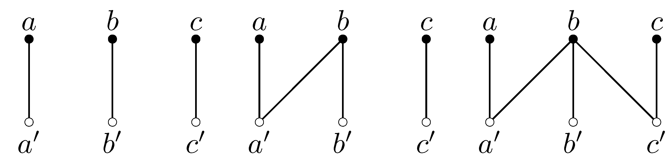
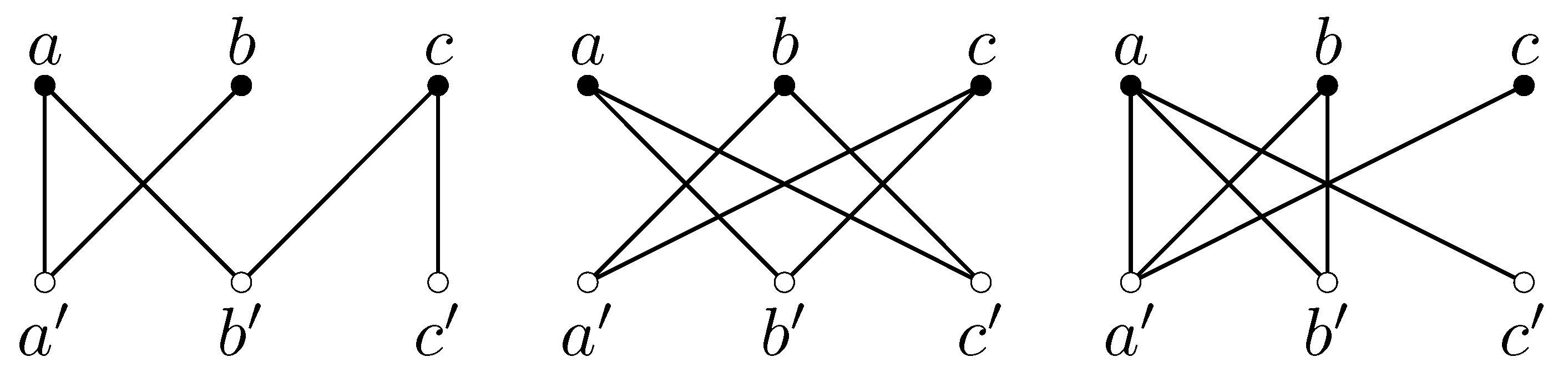
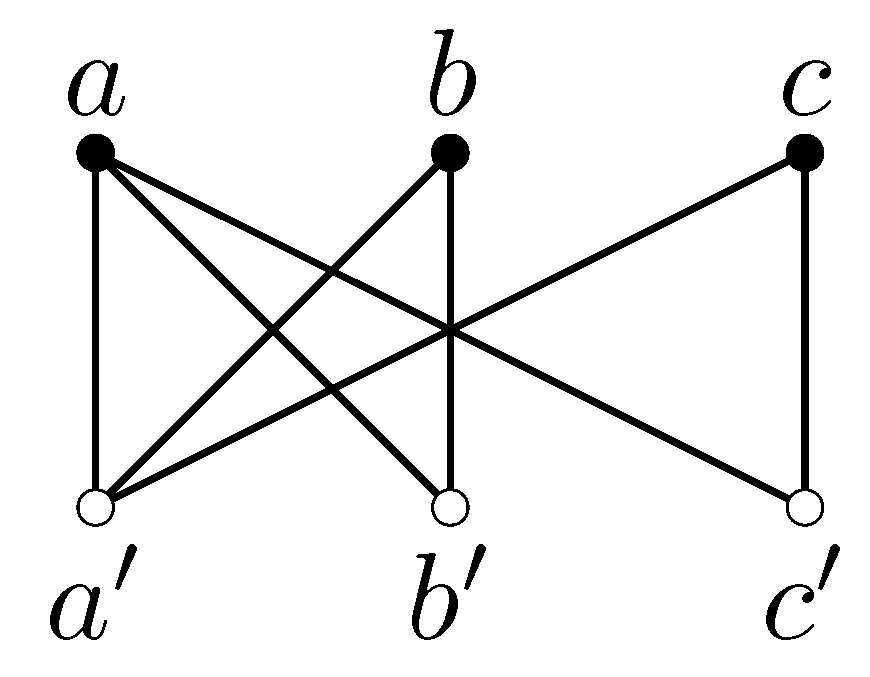
where ${\Omega }_Q\left(G\right)$ is the set of all induced bipartite subgraphs of G that are isomorphic to the graph Q, and ${\Omega }_{\mathcal{F}}\left(G\right)$ is the set of all induced bipartite subgraphs of G that are isomorphic to certain graph in the family $\mathcal{F}$. Here, ${\mathcal{F}}_1=\{2K_2,Q_7\},$ ${\mathcal{F}}_2=\{K_2,3K_2,K_2\cup P_4,P_6,Q_3,Q_6\},$ where $Q_3,Q_6$ and $Q_7$ are illustrated in Figure 1, Figure 2 and Figure 3.

Proof. 

From the proof of Theorem 1, we know that

$$det(\lambda I_{m+n}-M\left(H\right))=det(D^{\prime }+A^{\prime })=det\left(D^{\prime }\right)\sum _{\theta \subseteq [m+n]}{\displaystyle \frac{det\left(A_{\theta }^{\prime }\right)}{det\left(D_{\theta }^{\prime }\right)}}$$

(6)

where $H=K_{m,n}-G$, $A^{\prime }=A\left(H^{bc}\right)-{\mathbf{1}}_{V_1}{\mathbf{1}}_{V_2}^T-{\mathbf{1}}_{V_2}{\mathbf{1}}_{V_1}^T$, or

$$\begin{array}{c}{A}^{\prime }=\left[\begin{array}{cc}0& B\left(H^{bc}\right)-J_{m\times n}\\ B^T\left(H^{bc}\right)-J_{n\times m}& 0\end{array}\right].\hfill \end{array}$$

Hence we only need to study the summation

$$\sum _{\theta \subseteq [m+n]}{\displaystyle \frac{det\left(A_{\theta }^{\prime }\right)}{det\left(D_{\theta }^{\prime }\right)}}$$

(7)

or equivalently

$$1+\sum _{Q\in \mathcal{G}(K_{m,n}-G)}{\displaystyle \frac{{(-1)}^{\frac{\left|V\right(Q\left)\right|}{2}}{\left(det\left(B\right(Q\left)\right)\right)}^2}{\prod _{v\in V\left(Q\right)\cap X}((n-d_G\left(v\right))t+\lambda )\prod _{v\in V\left(Q\right)\cap Y}((m-d_G\left(v\right))t+\lambda )}}].$$

(8)

Observe that $r\left(A^{\prime }\right)=2r(B\left(H^{bc}\right)-J_{m\times n})\le 2r\left(B\left(H^{bc}\right)\right)+2r\left(J_{m\times n}\right)=2r\left(B\left(G\right)\right)+2=r\left(A\left(G\right)\right)+2\le 6$. The following cases need to be discussed: Case 1: If $\theta =\varnothing$, then

$${\displaystyle \frac{det\left(A_{\theta }^{\prime }\right)}{det\left(D_{\theta }^{\prime }\right)}}=1.$$

Case 2: If $\left|\theta \right|=2$, then

$$A_{\theta }^{\prime }=\left[\begin{array}{cc}0& 1\\ 1& 0\end{array}\right].$$

Consequently, $Q\cong K_2$ and $Q^{bc}\cong K_2^{bc}$ (the trivial graph on two vertices). The contribution of this case to the summation part of Eq. (7) is given by

$$\sum _{Q\in {\Omega }_{K_2}(K_{m,n}-G)}{\displaystyle \frac{-1}{\prod _{v\in V\left(Q\right)\cap X}((n-d_Q\left(v\right))t+\lambda )\prod _{v\in V\left(Q\right)\cap Y}((m-d_Q\left(v\right))t+\lambda )}}.$$

Case 3 If $\left|\theta \right|=4$, then $|\theta \cap [m\left]\right|=|\theta \cap [m+1,m+n\left]\right|=2$. Let $\theta =\{i,j,k,l\}$ with $i<j<k<l$, where $i,j\in \left[m\right]$ and $k,l\in [m+1,m+n]$. In this case, the matrix $A^{\prime }$ is in the form

$${A^{\prime }}_{\theta }=\left[\begin{array}{cccc}0& 0& a_{ik}& a_{il}\\ 0& 0& a_{jk}& a_{jl}\\ a_{ik}& a_{jk}& 0& 0\\ a_{il}& a_{jl}& 0& 0\end{array}\right],$$

where $\left[\begin{array}{cc}{a}_{ik}& a_{il}\\ a_{jk}& a_{jl}\end{array}\right]\mathrm{is}\mathrm{permutationally}\mathrm{equivalent}\mathrm{to}\left[\begin{array}{cc}1& 0\\ 0& 1\end{array}\right]\mathrm{or}\left[\begin{array}{cc}1& 1\\ 0& 1\end{array}\right]$ since $det\left(A_{\theta }^{\prime }\right)\ne 0$. This indicates that the induced subgraph Q in $K_{m,n}-G$ satisfies that $Q\cong 2K_2$ or $P_4$. The contribution of this case to the summation part of Eq. (7) is given by

$$\sum _{Q\in {\Omega }_{\{2K_2,P_4\}}(K_{m,n}-G)}{\displaystyle \frac{1}{\prod _{v\in V\left(Q\right)\cap V_1}((n-d_Q\left(v\right))t+\lambda )\prod _{v\in V\left(Q\right)\cap V_2}((m-d_Q\left(v\right))t+\lambda )}}.$$

Case 4 If $\left|\theta \right|=6$, then $|\theta \cap [m\left]\right|=|\theta \cap [m+1,m+n\left]\right|=3$. Suppose $B_3\left(Q^{bc}\right)$ is the $3\times 3$ principal submatrix of $B\left(Q^{bc}\right)$ in $A^{\prime }$ such that

$$A_{\theta }^{\prime }=\left[\begin{array}{cc}0& B_3\left(Q^{bc}\right)-J_3\\ {(B_3\left(Q^{bc}\right)-J_3)}^T& 0\end{array}\right].$$

Moreover,

$$det\left(A_{\theta }^{\prime }\right)={(-1)}^{3\times 3}det\left(B_3\left(Q^{bc}\right)-J_3\right)det\left({(B_3\left(Q^{bc}\right)-J_3)}^T\right)=-{(det(J_3-B_3\left(Q^{bc}\right)))}^2.$$

By exhaustive search, there exist 174 nonsingular 0–1 matrices of order 3, each of which is permutationally equivalent to one of the following seven matrices or their transposes:

$$B_1=\left[\begin{array}{ccc}1& 0& 0\\ 0& 1& 0\\ 0& 0& 1\end{array}\right],B_2=\left[\begin{array}{ccc}1& 0& 0\\ 0& 1& 1\\ 0& 0& 1\end{array}\right],B_3=\left[\begin{array}{ccc}1& 1& 0\\ 0& 1& 0\\ 0& 1& 1\end{array}\right],B_4=\left[\begin{array}{ccc}1& 1& 0\\ 0& 1& 1\\ 0& 0& 1\end{array}\right],$$

$$B_5=\left[\begin{array}{ccc}0& 1& 1\\ 1& 0& 1\\ 1& 1& 0\end{array}\right],B_6=\left[\begin{array}{ccc}1& 1& 1\\ 1& 1& 0\\ 1& 0& 0\end{array}\right],B_7=\left[\begin{array}{ccc}1& 1& 0\\ 1& 1& 1\\ 0& 1& 1\end{array}\right].$$

In [17], it is proved by the authors that $B_k$ corresponds to the induced subgraph $Q_k$ in $K_{m,n}-G$, where $Q_1\cong 3K_2$, $Q_2\cong K_2\cup P_4$, $Q_3$, $Q_4\cong P_6$, $Q_5\cong C_6$, $Q_6$, or $Q_7$ (see Figure 1, Figure 2 and Figure 3 ). By Lemma 1 or simple calculations, we know that $(det{(J_3-B\left(Q_k^{bc}\right))}^2=1$ for $k=1,2,3,4,6,7$ and ${(det(J_3-B\left(Q_5^{bc}\right)))}^2=4$. Hence, the contribution of this case to Eq. (7) is given by

$$\begin{array}{cc}\hfill & \sum _{Q\in {\Omega }_{\{Q_1,Q_2,Q_3,Q_4,Q_6,Q_7\}}(K_{m,n}-G)}{\displaystyle \frac{-1}{\prod _{v\in V\left(Q\right)\cap X}((n-d_Q\left(v\right))t+\lambda )\prod _{v\in V\left(Q\right)\cap Y}((m-d_Q\left(v\right))t+\lambda )}}\hfill \\ +\hfill & \sum _{Q\in {\Omega }_{C_6}(K_{m,n}-G)}{\displaystyle \frac{-4}{\prod _{v\in V\left(Q\right)\cap X}((n-d_Q\left(v\right))t+\lambda )\prod _{v\in V\left(Q\right)\cap Y}((m-d_Q\left(v\right))t+\lambda )}}.\hfill \end{array}$$

The proof is completed. □

5. Conclusions

In this paper we studied the computation of the generalized characteristic polynomial or equivalently the zeta function of graphs, and derived a general formula for the generalized characteristic polynomial of the $K_{m,n}$-complement of a bipartite graph. As a by-product, we obtained an explicit formula for the generalized characteristic polynomial of the $K_{m,n}$- tite complement of a bipartite graph with rank no more than 4. In a sense, the formulas obtained in this paper are straightforward and only rely on the use of fundamental linear algebra about the biadjacency matrix of the bipartite graph.

References

- D. Cvetković, S. K. D. Cvetković, S. K. Simić, Towards a spectral theory of graphs based on the signless Laplacian. Publ. Inst. Math. 85 (2009) 19–33.
- W. Linear Algebra Appl. 434 (2011) 1378–1387.
- O. Kada, Characteristic polynomials and zeta functions of equitably partitioned graphs. Linear Algebra Appl. 588 (2020) 471–488.
- L. Bartholdi, Counting paths in graphs, Enseign.Math. 45 (1999) 83–131.
- Y. Ihara, On discrete subgroups of the two by two projective linear group over p-adic fields. J. Math. Soc. Japan 18 (1966) 219–235.
- S. Northshield, A note on the zeta function of a graph. J. Combin. Theory Ser. B 74 (1998) 408–410.
- A. Terras, Zeta Functions of Graphs: A Stroll Through the Garden. Cambridge University Press, Cambridge (2011).
- I. Sato, Zeta functions and complexities of a semiregular bipartite graph and its line graph. Discrete Math. 307 (2007) 237–245.
- I. Sato, Zeta functions and complexities of middle graphs of semiregular bipartite graphs. Discrete Math. 355 (2014) 92–99.
- P. Graphs Combin. 29 (2013) 1633–1646.
- A. Blanchard, E. A. Blanchard, E. Pakala, M. Somodi, Ihara zeta function and cospectrality of joins of regular graphs. Discrete Math. 333 (2014) 84–93.
- H.Y. Chen, Y. H.Y. Chen, Y. Chen, Bartholdi zeta functions of generalized join graphs. Graphs Combin. 34 (2018) 207–222.
- H.K. Kim, J. H.K. Kim, J. Lee, A generalized characteristic polynomial of graphs having a semifree action. Discrete Math. 308 (2008) 555–564.
- B. Khodakhast, On the determinant of bipartite graphs. Discrete Math. 313 (21) (2013) 2446–2450.
- J.C. Bruce, Characteristic polynomials by diagonal expansion. Am. Stat. 37 (1983) 233–235.
- R.B. Bapat, Graphs and Matrices. Hindustan Book Agency & Springer, New Delhi, India (2010).
- H.L. Gong, Y. H.L. Gong, Y. Gong, J. Ge, The number of spanning trees in Kn-complement of a bipartite graph. J. Algebr. Combin. 2024. [Google Scholar]
- H. Bass, The Ihara-Selberg zeta function of a tree lattice. Internat. J. Math. 3 (1992) 717–797.
- D. Graphs Combin. 35 (2019) 1503–1517.