
Submitted:
06 December 2024
Posted:
09 December 2024
You are already at the latest version
Abstract
Aircraft envelope expansion during the installation of new underwing stores presents significant challenges, particularly due to the aeroelastic flutter phenomenon. Accurate modeling of aeroelastic behavior often necessitates flight testing, which poses risks due to the potential catastrophic consequences of reaching the flutter point. Traditional methods, like frequency sweeps, are effective but require prolonged exposure to flutter conditions, making them less suitable for transonic flight validations. This paper introduces a robust deep learning approach to process sine-dwell signals from aeroelastic Flutter Flight Tests, characterized by short data lengths (less than 5 seconds) and low frequencies (less than 10 Hz). We explore the preliminary viability of different deep learning networks and compare their performance to existing methods such as the PRESTO algorithm and Laplace Wavelet estimation. Deep learning algorithms demonstrate substantial accuracy and robustness, providing reliable parameter identification for flutter analysis while significantly reducing the time spent near flutter conditions. Although the results with the networks trained show less accuracy than the PRESTO algorithm but more than the Laplace Wavelet estimation, the results are promising enough to justify extended investigation on this area. This approach is validated using both synthetic data and real F-18 flight test signals, highlighting its potential for real-time analysis and broader applicability in aeroelastic testing.
Keywords:
Aeroelastic Flutter
; flight testing
; deep learning
; convolutional neural network
; deep neural network
; multilayer perceptron
; sine-dwell
; system identification
; damping
; natural frequency
; PRESTO algorithm
; Laplace wavelet Matching Pursuit
; real-time analysis
; aircraft envelope expansion
; real data analysis
1. Introduction
The validation of aircraft airworthiness during flutter flight tests is a critical step in expanding the flight envelope of new or modified aircraft designs, as outlined in [1,2]. These tests involve different steps, one of them being identifying aeroelastic flutter, a condition where aerodynamic forces couple with structural dynamics resulting in self-excited oscillations. One of the final steps during flutter testing is the analysis of signals captured during flight (at different flight conditions of dynamic pressure) to estimate parameters, such as natural frequencies and damping, essential to determining safe flight conditions at each point of the flight envelope.
Traditional methodologies, such as frequency sweeps, remain the most common approach in flutter flight tests [3]. These methods, often analyzed using the Rational Fraction Polynomials technique [4,5,6], have been augmented with advanced modal estimation techniques such as Polymax and Stochastic Subspace Identification (SSI) [7,8]. Although effective, these techniques require extensive time near flutter conditions, particularly during transonic regime testing, where aeroelastic behavior becomes highly nonlinear and less predictable [9,10]. This prolonged exposure increases safety risks and operational complexity.
An alternative to frequency sweeps is the use of sine-dwell excitations, which involve short-duration, low-frequency signals [3]. Although sine-dwell excitations offer significant advantages in minimizing the time spent near critical flutter conditions, their use in flutter analysis has been limited. Few authors have explored this approach in depth. Notable examples include Lind [11], who applied Laplace wavelet techniques to estimate modal parameters, and Barros-Rodriguez et al. [12], who utilized Singular Value Decomposition (SVD) filtering to address noise challenges. Mehra [13] used the Prony method for parameter identification, while Chabalko et al. [14] investigated the use of continuous wavelet transforms to analyze short-duration signals. A more recent method, the Power Spectrum Short Time Optimization (PRESTO) approach, was introduced in [15]. This technique begins with a rapid initialization of parameters using basic spectral analysis, which provides a robust starting point. It then refines these parameters through a time-domain optimization process employing a trust-region-reflective algorithm, ensuring precise and reliable results.
Although all of these methods have shown promise in specific applications, they face notable limitations, such as computational inefficiency, reduced accuracy in low signal-to-noise ratio environments, and difficulties in handling short data lengths characteristic of sine-dwell signals. These challenges underscore the need for innovative approaches to analyze such data effectively and reliably.
Deep Learning (DL) has emerged in recent years as a transformative tool in fields such as signal processing, image recognition, and system identification [16]. Convolutional Neural Networks (CNNs) and Deep Neural Networks (DNNs), in particular, have shown exceptional performance in handling complex, noisy datasets. However, their application in flutter flight testing remains largely unexplored. Although studies like [17,18,19] have utilized DL to classify flutter conditions or predict airspeed thresholds, the direct estimation of aeroelastic parameters from flight test data, especially sine-dwell signals, has received limited attention. Challenges such as adapting DL architectures to the specific nature of flutter data and ensuring robust performance with noisy, short-duration signals remain open research questions.
This paper proposes a novel application of DL techniques, including CNNs and DNNs, to process sine-dwell signals for accurate parameter identification in flutter testing. By leveraging synthetic datasets for training and comparing DL methods against established techniques such as PRESTO [15] and Laplace Wavelet estimation [11], we aim to demonstrate the feasibility and advantages of DL in this domain. The proposed approach addresses key limitations of existing methods, such as computational inefficiency and reduced accuracy in noisy environments, while paving the way for real-time in-flight analysis.
The remainder of this paper is organized as follows. Section 2 provides an overview of the materials and methods, detailing the generation of synthetic datasets, DL architectures, and evaluation metrics. Section 3 presents the experimental results, comparing DL methods with traditional approaches on both synthetic and real flight test data. Finally, Section 4 discusses the implications of these findings and outlines future directions for research in this area.
2. Materials and Methods
This section describes the methodology and resources used in the study. The aim is to evaluate the use of Deep Learning techniques for identifying aeroelastic flutter parameters from sine-dwell signals. The generation of synthetic datasets, the design of neural network architectures, and the evaluation metrics are explained. Comparisons with traditional methods such as the PRESTO algorithm and Laplace Wavelet Matching Pursuit estimation are also included as a reference.
PRESTO and Laplace Wavelet Matching Pursuit are similar processing techniques that rely on models described in standards [20,21], providing very accurate solutions. However, the application of Machine Learning in this field has been barely explored. To date, no study has specifically focused on identifying flutter-related parameters from flight test data.
Regarding recent investigations, [17] employed a method based on DNNs to predict flutter airspeed during the analysis phase, prior to flight testing. While their work focuses on pre-flight analysis, it does not address the direct identification of flutter parameters during flight.
In [18] and [19] the authors presented approaches that align more closely with the objectives of this paper by utilizing CNN models. Their methods were applied to data extracted from flight tests, although their validation was primarily conducted using wind tunnel test data. Instead of identifying system parameters, these studies classified conditions as either flutter or no flutter during flight.
Similarly, [22] applied a DNN to analyze flight test data. However, their study focused on modeling the global behavior of the structure rather than on identifying specific flutter parameters.
Perhaps the most comparable work is that of [23], who explored various techniques, including CNNs and Multi-Layer Perceptrons (MLPs), in the context of helicopter rotor blade applications. While their problem shares similarities with the present study, it does not involve the analysis of sine-dwell data.
The method proposed by the authors focuses on accurately identifying the flutter parameters of the aeroelastic equations of motion related to aeroelastic flutter. The main advantages of this method are that once trained, MLPs, DNNs, and CNNs provide almost immediate results using a low-end personal computer, which could enable effective real-time analysis. Additionally, if the training set includes a broad enough range of training parameters, it might be possible to identify accurate flutter parameters for a given number of modes, not just two.
The main limitation of this method is the need for a good and accurate model to provide reliable data. It is challenging to obtain reliable real flight data with accurate output parameters, for example, from Ground Vibration Tests. There is no public source of reliable data to match estimated mode values with the signals themselves. Instead, the signal model from [20] was used to generate synthetic training sets (and will be the model employed to fit the data and identify parameters) using Equation (1):
where N is the number of modes, is a constant representing amplitude, is the damping factor, represents the natural angular frequency of the structure, t is the time variable, is the damped angular frequency, represents the phase angle, and accounts for structural and aerodynamic noise.
The parameters that need to be identified for the characterization of the aeroelastic behavior of the j-th mode are the amplitude , the damping factor , the natural angular frequency and the phase angle .
Even though this model may seem simplistic by assuming a linear relationship between various factors (aerodynamic and other linear and non-linear interactions, such as gaps, hysteresis from structural damping, etc.) that are not properly modeled in Equation (1), [20] ultimately calls for monitoring two main parameters: modal frequency and damping for the critical flutter modes. Assuming that the mechanism responsible for flutter can be modeled by a second-order linear Ordinary Differential Equation (ODE), all interactions are reduced to Equation (1).
It is important to note that the authors are not dismissing the significance of other non-linear interactions with the natural modes by assuming that the second-order linear ODE will govern the flutter mechanism. These interactions will influence the approach to the flutter phenomenon, either accelerating or delaying flutter onset, which is crucial given the severe consequences of reaching a flutter point. This limitation must be considered when applying any analysis technique. Experienced engineers shall develop a sensible test plan based on all available information, noting that the methodology described in this paper will not provide information on flutter onset.
Considering all caveats and limitations, the potential of this technique is substantial, and it is worth exploring to develop accurate trained networks with the described advantages.
2.1. Input layer
We will differentiate two processes for adapting the input data, depending on the network type: MLP-based (including MLPs and DNNs) and CNNs.
2.1.1. MLP-based Networks input layer
The adaptation process for MLP-based networks is illustrated in Figure 1. The initial dataset consists of a time signal extracted from one of the aircraft sensors, typically a signal sampled at . However, the time length may vary depending on the expected modal frequencies of the critical flutter modes.
The following algorithm is followed:
- A Discrete Fourier Transform (DFT) is applied to the temporal signal, and the real and imaginary parts are separated.
- From each subset, 70 frequency samples are extracted (corresponding to a maximum frequency of if signals are used).
- The positive sections of both the real and imaginary components of the DFT are then concatenated.
This process results in a new signal, 140 samples long, comprised of the concatenated real and imaginary parts of the DFT, which will be used as input for the MLP-based network.
2.1.2. CNN Networks Input Layer
In the case of CNNs we need to follow a different approach. A matrix of input data is required instead of a vector.
The starting dataset is the same as for MLP-based networks, and in order to convert it into a 2D matrix we need to perform the following preprocessing operations:
- Define a list of unitary vectors on the complex plane, which will constitute the basis for a vector space , defined by a set of vectors . Each vector is calculated as:where k is the index of the vector, K is the total number of vectors (in this application, , which includes 14 unitary vectors, the real part, and the imaginary part), and represents the frequency datapoints. These vectors are equally distributed around the circumference. See Figure 2.
- Limit the original time series signal to samples, or zero-pad until of signal are reached.
- Calculate the DFT of the time series. The result is a vector with 200 elements defined on the base B.
- Select the first 70 datapoints, which correspond to a maximum frequency of .
- Project each frequency vector on the vector space defined in step 1 above. The projection values will be used as redundant information, and the 16 projection values will constitute the rows of the input matrix. See Figure 2.
At last, the input will be a matrix including redundant information.
2.2. Output Layer
In all cases the output layer will consist of 4 neurons, which correspond to the natural frequencies and damping factors of the two modes analyzed (2 natural frequencies and 2 damping factors).
Note that the original parameter list to be identified also includes an amplitude and phase angle for each mode. These amplitudes and phase angles have been estimated using a classical matching pursuit process [24].
2.3. Networks Design
We will utilize three different types of neural networks: MLPs, DNNs and CNNs. While detailed descriptions of each network are beyond the scope of this paper, readers can refer to [16] for foundational information.
2.3.1. Multi-Layer Perceptron Design
The MLPs consist of an input layer with 140 neurons, one hidden layer with a different number of neurons for each network, and an output layer with 4 neurons. The hidden layer employs the sigmoid activation function, enabling non-linear transformations and capturing complex patterns within the data. A diagram of these networks can be seen in Figure 3.
In this paper, the number following each MLP designation specifies the number of neurons in the hidden layer. For example, MLP 20 indicates 20 neurons in the hidden layer.
2.3.2. Deep Neural Networks Design
DNNs are an extension of the MLP networks. In this case, the network comprises more than one hidden layer, but follows exactly the same approach as MLP networks in Section 2.3.1 above. An example of the DNN design can be found in Figure 4. As in the case of the MLPs, our application will also consider 140 input samples and 4 outputs, with a different number of hidden layers. Again, the activation function selected for the hidden layers is the sigmoid function.
In the case of DNNs, the DNN designation will indicate the number of hidden layers and the number of neurons in each hidden layer. For example, DNN 2x20 indicates a DNN with 2 hidden layers and 20 neurons in each hidden layer.
2.3.3. Convolutional Neural Networks Design
CNNs are similar to DNNs in that they both consist of multiple hidden layers. However, the primary difference lies in how they compute the output parameters. CNNs use a convolution operation between the input matrices and the different layer parameter matrices, unlike DNNs that rely on compositions of linear transformations. The complete block diagram of a CNN with two hidden layers is depicted in Figure 5. Although there are various CNN architectures, the one used in this paper is detailed below, in one example with two hidden layers. Each layer involves different steps. The process applied to our system is as follows:
- Input Layer. The inputs are matrices for each dataset, which need to be in a format that represents a regular pattern, typically an image. In our case, the input is a data matrix as described in Section 2.1.2. So, the input layer will consist of neurons.
-
Convolutional process. Each convolutional process, depicted in Figure 5 as an elliptic box, includes a convolutional layer followed by several processes to enhance the operation quality:
- (a)
- Convolutional Layer. This layer performs the convolution operation on the input matrix using the weights matrix.
- (b)
- Normalization Process. This step normalizes the outputs to control their range and prevent saturation. A bias is added, and a multiplier is applied. These parameters are adjusted during training.
- (c)
- Rectification Process. This step converts negative values to zero.
- (d)
- Pooling Process. The convolutional matrices are downsampled using smaller windows.
- Connection Layer. This layer connects and reduces all outputs from the final convolutional block to the four output parameters. It functions as a classical perceptron layer, collecting outputs from the convolutional layers and producing an output to solve the regression problem.
- Regression Layer. Before returning the final parameters, a regression layer is applied to refine the outputs.
This example illustrates a CNN with two hidden convolutional blocks. However, more or fewer blocks can be used. In this paper, the trained CNNs employ 5 and 6 hidden layers for different networks.
In the case of CNNs, the designation includes the number of convolutional blocks and the number of neurons in each convolutional layer within the convolutional blocks. For example, CNN 5x100 indicates a Convolutional Neural Network with 5 convolutional processes and 100 neurons in each convolutional layer of each convolutional process.
2.4. Training Process
The training signals were synthetically generated using Equation (1), with parameters randomly sampled from Table 1. The training process was carried out using backpropagation on a computing cluster provided by the Universidad de Alcalá, utilizing MATLAB for implementation.
The noise in the training dataset was modeled as white noise with a signal-to-noise ratio (SNR) of 5 dB, using random seeds to generate unique noise profiles for each signal. Additionally, a separate synthetic dataset, independent of the training dataset, was created to evaluate the testing process. A comprehensive summary of the training dataset distribution is presented in Table 2, while details of the DNN techniques and architectures explored are outlined in Table 3.
During the training process, we also took into account several additional considerations:
- Signal Ranges: The limited range of frequencies is due to the preliminary nature of this study and the long times required for the networks to be trained. A broader range of frequencies, representative of the frequencies found in the real data available, will be employed in future papers, possibly including a different network design.
-
Dampings Upscaling: The dampings have been upscaled by a factor of 15 to reach a range of values in the same order of magnitude as the rest of the parameters. The formula employed is as follows:After the estimation is finished, it will be necessary to adjust the damping results inversely.
2.5. Analysis Methodology
To study the results we carried out two sets of experiments, one with synthetic data, and another with real data:
- Synthetic data processing: A set of synthetic signals dataset will be created with known parameters and no noise addition. Taking this dataset as a baseline, and following the same approach as with the training dataset, 5dB SNR white noise was added. The synthetic process will measure the standard deviations of errors in parameters (frequency and damping), skewness, kurtosis and histograms of errors.
- Real data processing: A set of real data from F-18 flutter tests will be employed. The sets will be analyzed by all the techniques, the data will be reconstructed using equation 1 with the estimated parameters and plotted the results of the original vs. the reconstructed data. From there, the Mean Square Error (MSE), the Mean Absolute Error (MAE) and the Maximum Absolute Error (MaxAE), along with the regression coefficients (, slope and y-intercept) will be compared.
3. Results
This section presents the experimental results, DL methods with traditional approaches on both synthetic and real flight test data. After processing the data, the following key results are obtained:
3.1. Synthetic Data Processing
As described in Section 2.4, several processing techniques were employed. All the DNNs were compared to Laplace Wavelet Matching Pursuit processing [11] and PRESTO processing [15] as reference. Table 4 shows the results for a SNR of 5dB, considering the case closest to the real conditions. The analysis of this table shows several interesting facts.
PRESTO and Laplace Wavelet Matching Pursuit were added to the analysis for comparison. PRESTO returns the highest standard deviation compared to the other neural networks average for frequency ( higher) and damping ( higher). However is strongly leptokurtic, noticeably above the rest of the methods also (4 points above for frequency and 30 points above for damping). Regarding skewness coefficient, even though is the only method that returns a negative skewness in frequency is still within limits of symmetry, like the rest of the methods. However in damping the skewness is also the highest of the techniques. Even though most are skewed to the left given the negative coefficient, PRESTO shows the highest skewness of all. The conclusion is that PRESTO returns more accurate results than the neural networks techniques, at the price of the most extreme outliers and a long processing time ( orders of magnitude).
On the other hand, Laplace Wavelet Matching Pursuit returns similar values to the rest of the neural networks methods. Even though in frequency the standard deviation is higher than the rest of the neural networks ( higher) in damping is below the average, specifically around the same values as the rest of the CNNs (several of the DNNs increase the average substantially). In kurtosis, in frequency and damping is more leptokurtic than the average ( points above in frequency, including CNNs, and 2 points above in damping, although below than the CNNs). At last, the frequency skewness is substantially low, one order of magnitude below the average, indicating a strongly symmetric distribution as compared to the rest of the methods, and in damping is also skewed to the left, although in the average as compared to the rest of the methods. The conclusion is that is a method similar to the rest of the neural networks processed, although the nominal processing time is also orders of magnitude higher than the neural network techniques, a caveat needs to be expressed. To achieve a similar accuracy as the rest of the techniques, it was necessary to fine tune the dictionaries to the data searched, limited to be the smallest as possible given that the computers used ran out of memory with higher dictionaries. If the ranges f the dictionaries were the same as for PRESTO, the processing time was estimated to increase in at least 3 more orders of magnitude (meaning 6 orders of magnitude above the neural networks techniques). This fact may also account for the relatively low values for standard deviation, although cannot be confirmed.
Figure 6 shows a comparison between the error histograms of PRESTO, Laplace Wavelet Matching Pursuit, a CNN of 100 x 6 and a DNN of 100 x 100 x 100 as a samples for comparison, taking into account that the rest of the neural network processing techniques show a similar behavior. The plot shows a very similar distribution for the CNN and Laplace, sensibly better for the CNN damping and frequency, and slightly worse for the DNN frequency.
3.2. Real Data Processing
A set of F-18 flutter flight tests data, from the Spanish Air Force CLAEX, was processed and analyzed by the aforementioned techniques. Table 5 shows the results of the analysis process.
The dataset was comprised of 640 signals, extracted from 10 extensometers (6 torsion and 4 bending), 8 flight envelope test points and also 8 excitation frequency runs for each test point (totaling 640 signals). Note that in real life rarely pure bending-torsion flutter modes appear. Usually the nodes lines are not parallel and perpendicular to the cord line, but hold particular shapes, and therefore it is common to see energy from both modes in each sensor. However, approximately only to of the 640 signals carried information related to the natural modes of the structure, since during the sine-dwell runs the frequencies are changed with every excitation. Depending on the natural modes frequencies and the frequency of that test run, it may be possible to catch the energy from one, two or three excitation runs. Rarely more than that.
Considering the aforementioned, even though the 640 signals were analyzed only the 150 best signals participated of the statistics in Table 5. The original data was processed by the different techniques and the signals reconstructed from the parameters estimated. Then, the original signal values were assigned to the x axis while the reconstructed signals values were assigned to the y axis, generating a scatter plot of original vs. reconstructed data (Figure 7) and allowing to calculate regression metrics.
The analysis of the data allows to draw several conclusions. In general, the behavior of the DL techniques on real data is similar to the results on synthetic data, as is globally slightly worse than PRESTO but similar or slightly better than Laplace. It does not constitute a validation of the synthetic results, but is significant. Another conclusion is that all the DNN techniques show a similar behavior. The comparison between different deep learning techniques will be focused on the relationship between m (slope of the regression curve), and the different error metrics. Note that even though all the confidence intervals overlap, and therefore these differences cannot be assumed significant, there is a consistent trend in the averages of all the metrics for ones above the others. In general the error metrics show similar results for DNNs and MLPs, and slightly higher for CNNs, while the regression metrics show the opposite trend.
Comparing the DL results with Laplace, the aforementioned conclusions can be extrapolated also. Assuming only the average values and ignoring the confidence intervals, Laplace could be positioned between CNNs and MLPs, very similar to DNNs. However, the results for PRESTO are sensibly higher than the rest of the techniques, out of confidence intervals. In this case, given that the average values of the CNN techniques are located consistently in the upper bound of the rest of the techniques, the distance with PRESTO is lower than the rest, although not specially significant. This behavior is consistent among all the error metrics and regression coefficients. The slope is closer to 1 in PRESTO, meaning that the large values of amplitude are better fit, the error metrics for PRESTO are lower also, meaning that the lower values in amplitude don’t represent a biased fit (for example, if one method tends to fit higher values but ignores lower, then those errors end up accumulating in the error metrics). There is also no significant difference between the MSE and MAE in between methods, meaning that no significant outliers impacted the processing in one method before another, which is confirmed by a similar trend with MaxAE.
4. Discussion
The results presented in this study indicate that, although the PRESTO technique currently outperforms Deep Learning methods in terms of accuracy, the latter show significant potential for analyzing sine-dwell excitations during flutter tests. This represents a promising advance, in particular for transonic regime envelope expansion. The main advantage of Deep Learning techniques lies in their extraordinary short processing times compared to PRESTO and Laplace Wavelet Matching Pursuit. This makes them highly suitable for real-time analysis during flight tests, where rapid decision-making is critical.
When comparing the Deep Learning techniques, no single method demonstrated a clearly superior performance. While the increased complexity of CNNs led to slightly better results in some cases, the necessity to artificially construct a input matrix with redundant data probably impacted the benefits of this architecture. Consequently, the improvements in accuracy were not proportional to the additional architectural complexity, as seen when comparing the performance of the simplest MLP configuration (20 neurons) with the most sophisticated CNN, which did not yield the expected gains in performance.
This observation suggests that further refinement of the architecture is necessary. Modifications may include redesigning the input and output layers to better capture the relationships between parameters or adopting a multi-network approach. For example, individual networks could be dedicated to identifying specific parameters, and their outputs could be integrated into a higher-level network along with the input data. This hierarchical approach would resemble the iterative structure of the PRESTO technique, potentially leading to more accurate and efficient parameter identification.
5. Conclusions
This study explored the application of Deep Learning techniques for identifying aeroelastic flutter parameters from sine-dwell excitations, presenting a potential alternative to traditional methods such as PRESTO and Laplace Wavelet Matching Pursuit. The findings highlight several advantages and challenges associated with these modern approaches.
Deep Learning techniques, particularly MLPs, DNNs, and CNNs, demonstrate significant potential due to their extraordinarily short processing times, which entitles them as a promising solution for real-time analysis during flight tests, in particular during the transonic regime, where the numerical models cannot provide a reliable estimation of the aeroelastic behavior. However, in terms of accuracy, currently the traditional PRESTO method currently outperforms the evaluated Deep Learning models (although the performance is similar, or slightly better, than Laplace Wavelet Matching Pursuit). This highlights the necessity of further refinement before Deep Learning can fully replace established methods.
The analysis revealed no substantial differences in accuracy among the tested Deep Learning architectures, despite the varying levels of complexity. For exampla, while CNNs showed slightly better results in some cases, their higher computational demands and the need for redundant input data limited their overall effectiveness. This lack of a clear performance advantage among architectures suggests that the current designs may not be fully optimized for the specific challenges posed by flutter parameter identification.
To address these limitations, future work should focus on redesigning the input and output layers of the networks, potentially adopting a multi-network architecture. Specialized networks dedicated to identifying specific parameters, followed by a higher-level network to integrate these results, could improve accuracy and efficiency.
Author Contributions
The authors contributed with the following aspects:
- Conceptualization:RobertoGil-Pita,SamiAbou-Kebeh
- Methodology:SamiAbou-Kebeh
- Software:SamiAbou-Kebeh,RobertoGil-Pita
- Validation:ManuelRosa-Zurera,RobertoGil-Pita
- Formal analysis:ManuelRosa-Zurera
- Investigation:SamiAbou-Kebeh
- Resources:ManuelRosa-Zurera
- Data curation:RobertoGil-Pita
- Original draftpreparation:SamiAbou-Kebeh
- Review andediting:RobertoGil-Pita,ManuelRosa-Zurera
- Visualization:SamiAbou-KebehLLano
- Supervision:RobertoGil-Pita,ManuelRosa-Zurera
- Projectadministration:RobertoGil-Pita
- Funding acquisition:ManuelRosa-Zurera
Funding
This work was funded by the Spanish Ministry of Science and Innovation under Project PID2021-129043OB-I00 (funded by MCIN/AEI/ 10.13039/501100011033/FEDER, EU), and by the Community of Madrid and University of Alcalá under project EPU-INV/2020/003.
Data Availability Statement
The data employed in this paper belongs to the Spanish Air Force. The authors were authorized to use the data with restrictions for research purposes
Acknowledgments
The authors show their appreciation to the Spanish Air Force for the authorization to employ the data used for this paper.
Conflicts of Interest
The authors declare no conflict of interest.
Abbreviations
The following abbreviations are used in this manuscript:
| 2D | 2 Dimensions |
| CLAEX | Centro Lgistico de Armamento y Experimentacion (as Spanish acronym) |
| CNN | Convolutional Neural Network |
| dB | Decibel |
| DFT | Discrete Fourier Transform |
| DL | Deep Learning |
| DNN | Deep Neural Network |
| Hz | Hertzs |
| Kurt. | Kurtosis coefficient |
| m | Slope of the regression curve |
| MAE | Mean Absolute Error |
| MaxAE | Maximum Absolute Error |
| MLP | Multilayer Perceptron |
| ms | Milliseconds |
| MSE | Mean Square Error |
| n | y-intercept of the regression curve |
| ODE | Ordinary Differential Equation |
| PRESTO | Power Spectrum Short Time Optimization |
| Skew. | Skewness coefficient |
| SNR | Signal to Noise Ratio |
| SSI | Stochastic Subspace Identification |
| Std. | Standard Deviation |
| SVD | Singular Values Decomposition |
References
- MIL-HDBK-516C. Airworthiness Certification Criteria. Technical Report December, DoD, 2014.
- EASA. CS-25. Certification Specifications and Acceptable Means of Compliance for Large Aeroplanes.
- J. Norton, W. J. Norton, W. AFFTC-TIH-90-001. Structures Flight Test Handbook. Technical Report November, USAF Test Pilot School, 1990.
- Formenti, D.; Richardson, M. Paramenter Estimation from Frequency Response Measurements Using Rational Fraction Polynomials. 1st IMAC Conference, 1982, pp. 1–10.
- Formenti, D.; Hill, M. Paramenter Estimation from Frequency Response Measurements Using Rational Fraction Polynomials (Twenty Years of Progress). 20th International Modal Analysis Conference (IMAC-20), 2002, pp. 1–10.
- Coll, F. JFlutter. Real Time Flutter Analysis in Flight Test. SFTE-EC; SFTE, SFTE: Nuremberg, 2016. [Google Scholar]
- Peeters, B.; Van des Auweraer, H. PolyMAX A Revolution in Modal Parameter Estimation. Proceedings of the 1st international Operational Modal Analysis Conference;, 2005; pp. 26–27.
- PEETERS, B.; DE ROECK, G. Reference-Based Stochastic Subspace Identification for Output-Only Modal Analysis. Mechanical Systems and Signal Processing 1999, 13, 855–878. [Google Scholar] [CrossRef]
- Volkmar, R.; Soal, K.; Govers, Y.; Böswald, M. Experimental and operational modal analysis: Automated system identification for safety-critical applications. Mechanical Systems and Signal Processing 2022, 183. [Google Scholar] [CrossRef]
- Govers, Y.; Mai, H.; Arnold, J.; Dillinger, J.K.; Pereira, A.K.; Breviglieri, C.; Takara, E.K.; Correa, M.S.; Mello, O.A.; Marques, R.F.; Geurts, E.G.; Creemers, R.J.; Timmermans, H.S.; Habing, R.; Kapteijn, K. Wind tunnel flutter testing on a highly flexible wing for aeroelastic validation in the transonic regime within the HMAE1 project. International Forum on Aeroelasticity and Structural Dynamics 2019, IFASD 2019 2019, pp. 1–25.
- Lind, R.; Brenner, M.; Freudinger, L.C. Wavelet Applications for flight flutter testing. CEAS/AIAA/ICASE/NASA Langley International Forum on Aeroelasticity and Structural Dynamics; Whitlow Jr., W., Ed. NASA, 1999, pp. 393–402.
- Barros-Rodriguez, J. Metodología de Ejecución y Explotación de los Ensayos en Vuelo de Flameo. PhD thesis, Universidad Politecnica de Madrid, 2014.
- Mehra, R.K.; Mahmood, S.; Waissman, R. Identification of Aircraft and Rotorcraft Aeroelastic Modes Using State Space System Identification. Proceedings of International Conference on Control Applications, 1995, pp. 432–447. [CrossRef]
- Chabalko, C.C.; Hajj, M.R.; Silva, W.A. Interrogative Testing for Nonlinear Identification of Aeroelastic Systems. AIAA Journal 2008, 46, 2657–2658. [Google Scholar] [CrossRef]
- Abou-Kebeh, S.; Gil-Pita, R.; Rosa-Zurera, M. Multimodal Estimation of Sine Dwell Vibrational Responses from Aeroelastic Flutter Flight Tests. Aerospace 2021, Vol. 8, Page 325 2021, 8, 325. [Google Scholar] [CrossRef]
- Goodfellow, I.; Bengio, Y.; Courville, A. Deep Learning; Number 1-2, The MIT Press, 2017.
- Wang, Y.R.; Wang, Y.J. Flutter speed prediction by using deep learning. Advances in Mechanical Engineering 2021, 13, 1–15. [Google Scholar] [CrossRef]
- Zheng, H.; Wu, Z.; Duan, S.; Zhou, J. Feature Extracted Method for Flutter Test Based on EMD and CNN. International Journal of Aerospace Engineering 2021, 2021, 10. [Google Scholar] [CrossRef]
- Duan, S.; Zheng, H.; Liu, J. A Novel Classification Method for Flutter Signals Based on the CNN and STFT. International Journal of Aerospace Engineering 2019, 2019, 1–8. [Google Scholar] [CrossRef]
- MIL-A-8870C. Military Specification: Airplane Strength and Rigidity. Vibration, Flutter and Divergence. Technical Report March, DoD, 1993.
- JSSG-2006. Joint Service Specification Guide. Aircraft Structures. Technical report, DoD, 1998.
- Li, K.; Kou, J.; Zhang, W. Deep neural network for unsteady aerodynamic and aeroelastic modeling across multiple Mach numbers. Nonlinear Dynamics 2019, 96, 2157–2177. [Google Scholar] [CrossRef]
- Chatterjee, T.; Essien, A.; Ganguli, R.; Friswell, M.I. The stochastic aeroelastic response analysis of helicopter rotors using deep and shallow machine learning. Neural Computing and Applications 2021, 33, 16809–16828. [Google Scholar] [CrossRef]
- Goodwin, M. Matching pursuit with damped sinusoids. 1997 IEEE International Conference on Acoustics, Speech, and Signal Processing. IEEE Comput. Soc. Press, 1997, Vol. 3, pp. 2037–2040. [CrossRef]
Figure 1.
MLP and DNN data preparation diagram.
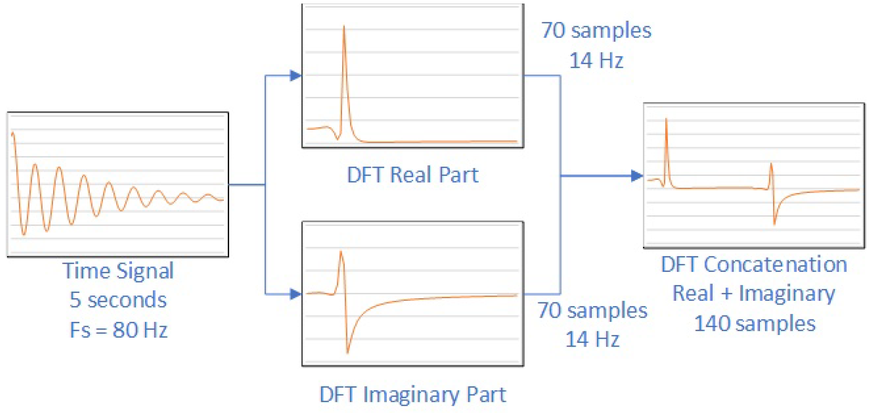
Figure 2.
Construction of the input matrix to feed the CNN. Once the time series dataset is transformed into a complex frequency spectrum, each point (example in blue) will be defined on the base B (in red) and projected onto the vector space V (in black). Note that the unit vectors .
Figure 2.
Construction of the input matrix to feed the CNN. Once the time series dataset is transformed into a complex frequency spectrum, each point (example in blue) will be defined on the base B (in red) and projected onto the vector space V (in black). Note that the unit vectors .
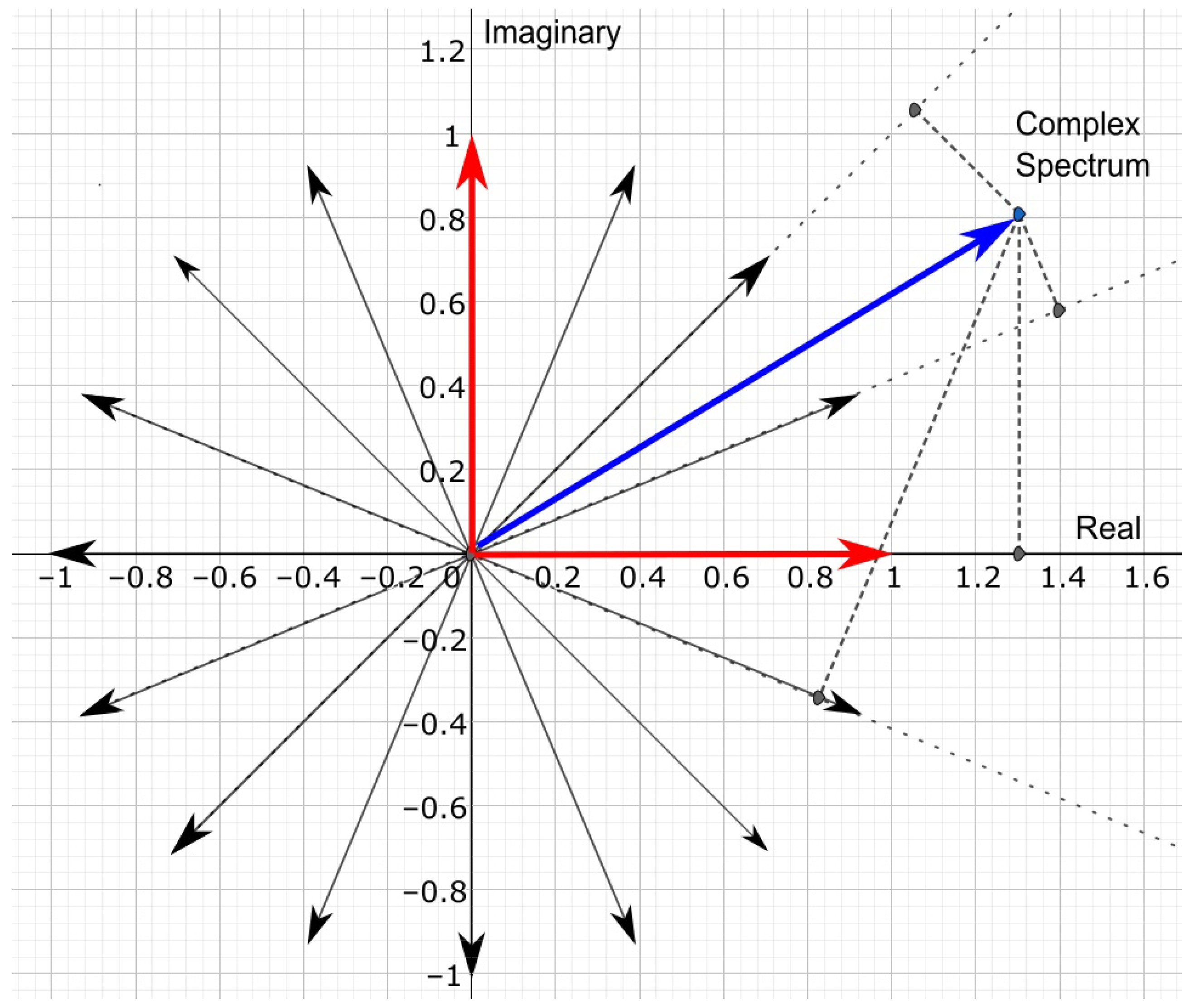
Figure 3.
Multi Layer Perceptron sample network diagram. In this case the MLP with 20 neurons in the hidden layer is depicted.
Figure 3.
Multi Layer Perceptron sample network diagram. In this case the MLP with 20 neurons in the hidden layer is depicted.
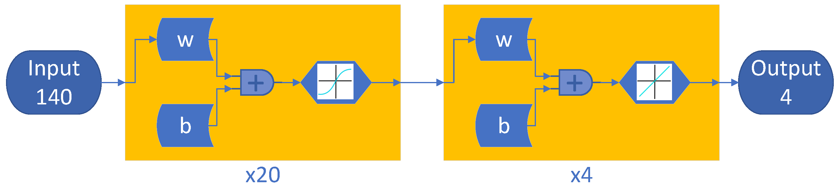
Figure 4.
DNN sample. In this case a DNN with one input layer, three hidden layers and one output layer is depicted. In this case each hidden layer has 40 neurons.
Figure 4.
DNN sample. In this case a DNN with one input layer, three hidden layers and one output layer is depicted. In this case each hidden layer has 40 neurons.
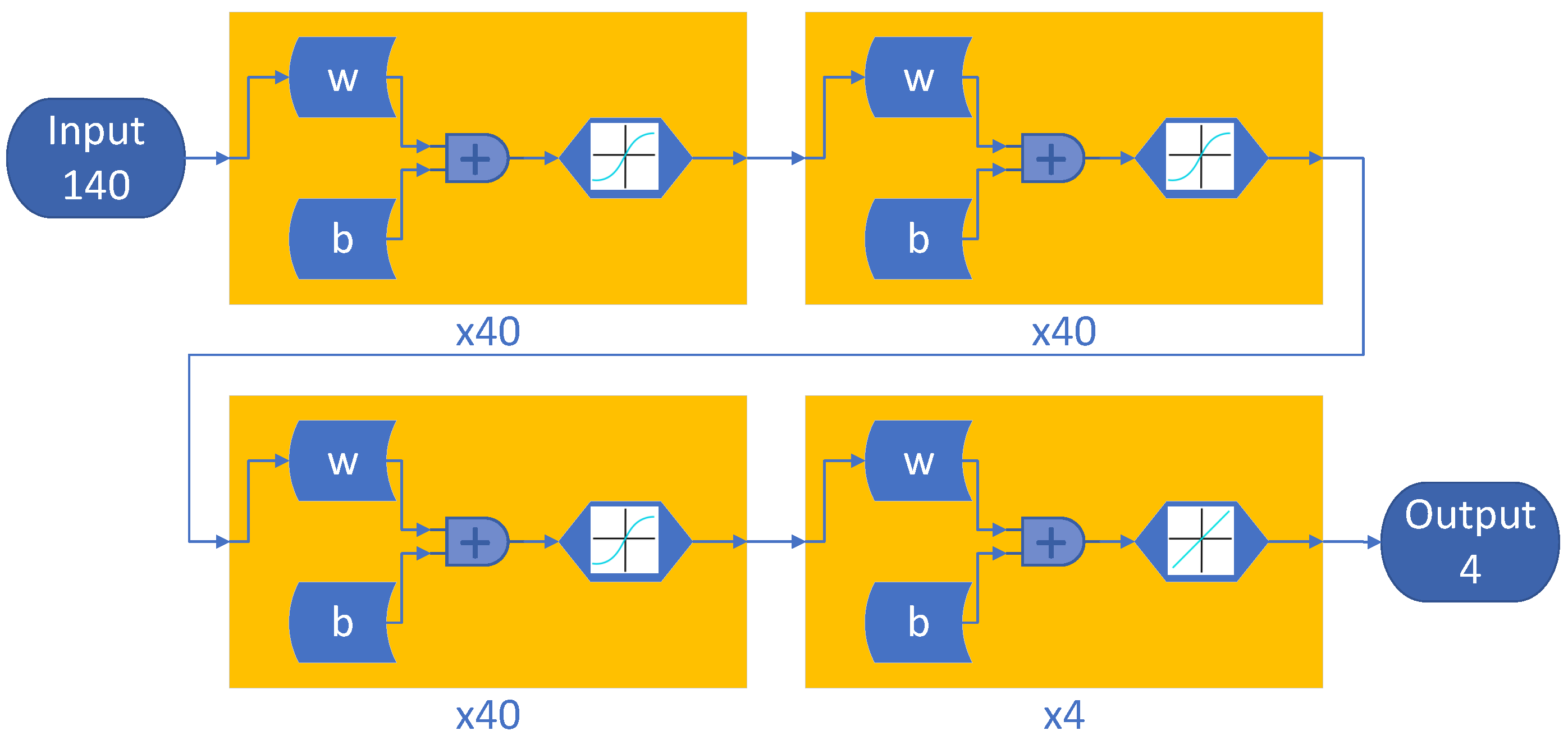
Figure 5.
Sample CNN. This example shows a CNN with one input layer, two convolutional layers, one connection layer, and one regression layer. Each convolutional layer has a different number of neurons and convolutional processes.
Figure 5.
Sample CNN. This example shows a CNN with one input layer, two convolutional layers, one connection layer, and one regression layer. Each convolutional layer has a different number of neurons and convolutional processes.
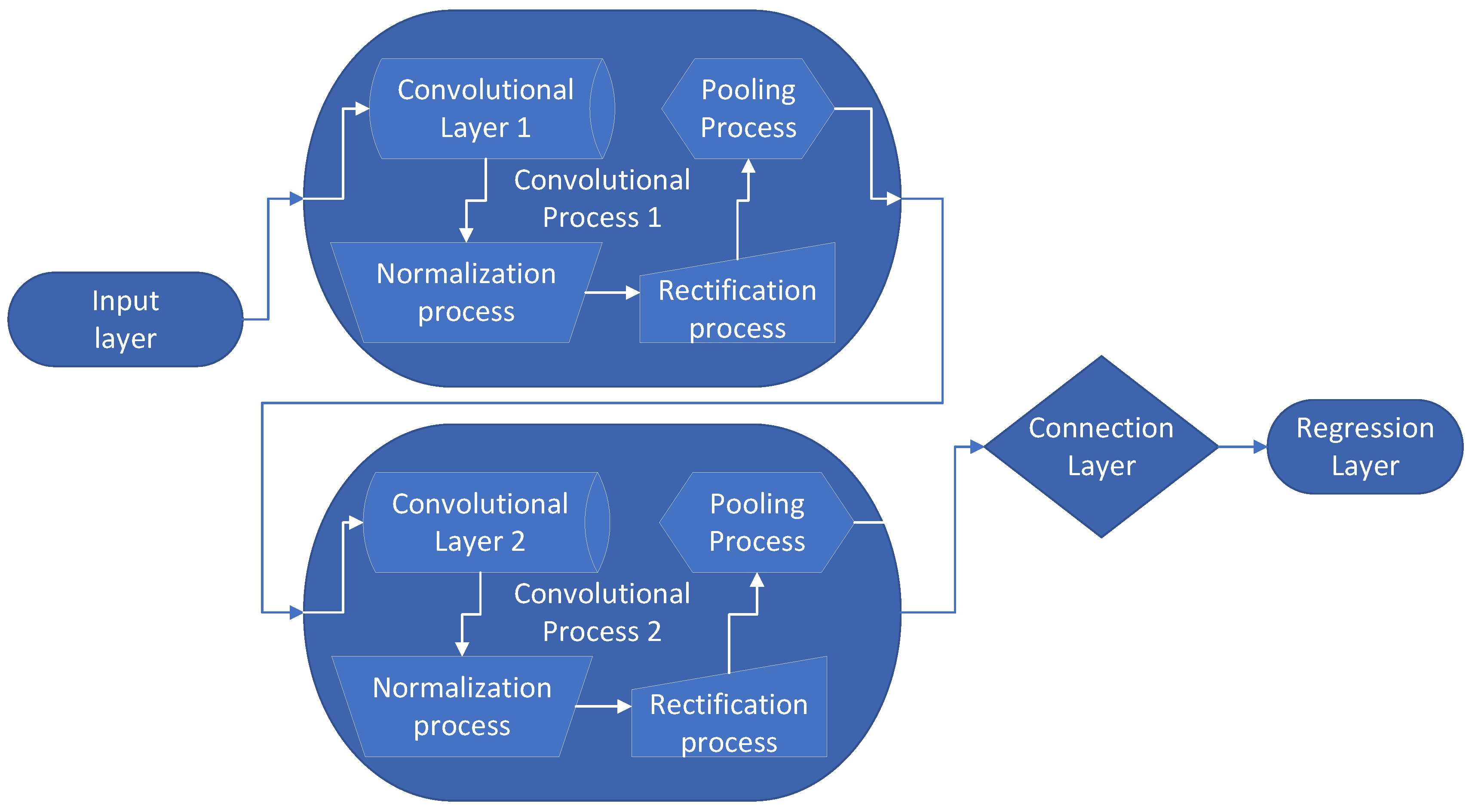
Figure 6.
Error histograms for frequency and damping for PRESTO, Laplace Wavelet Matching Pursuit, CNN 100 x 6 and DNN 100 x 100 x 100 chosen as sample methods. The rest of the neural network methods show a similar distribution to the ones depicted here. The plot for damping in the PRESTO method was truncated at relative damping, since the tail reached .

Figure 7.
Scatter plot comparing the regression curves of real data vs. synthetic reconstructed data. Comparison between Laplace Wavelet Matching Pursuit, PRESTO and a CNN 100 x 6 taken as a sample method.
Figure 7.
Scatter plot comparing the regression curves of real data vs. synthetic reconstructed data. Comparison between Laplace Wavelet Matching Pursuit, PRESTO and a CNN 100 x 6 taken as a sample method.
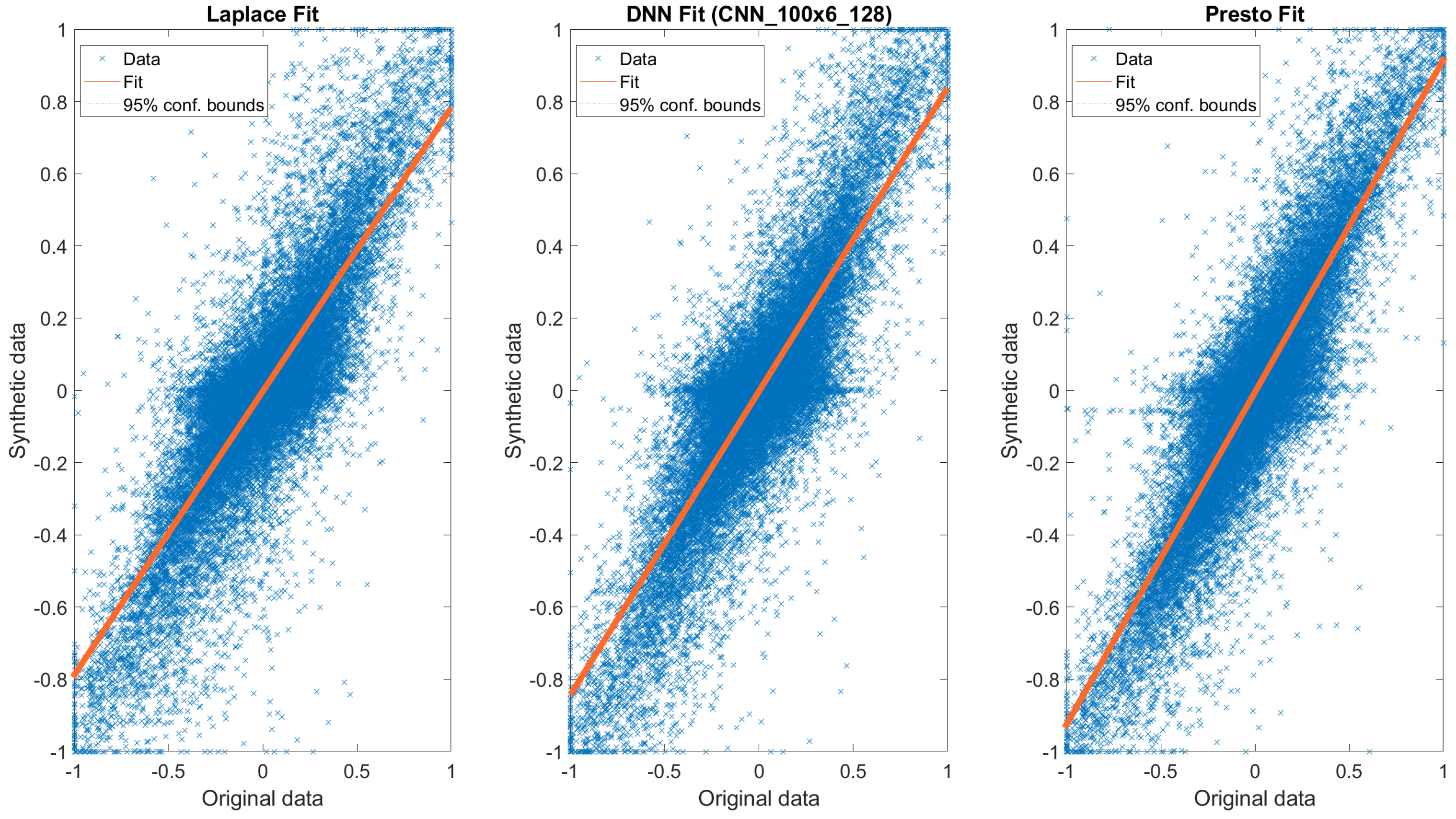

Table 1.
Signal parameters ranges.
| Parameter Ranges | |
|---|---|
| Frequency ranges | 4Hz - 6Hz |
| Damping ranges | 0.01 - 0.2 |
| Phase ranges | 0 rad - 2 rad |
| Amplitude ranges | 0 - 1 |
| Other Characteristics | |
| Dampings | Upscaled by a factor of 15 |
Table 2.
Distribution of training datasets.
| Total | ||
|---|---|---|
| Combined training signals | 300,000 | |
| Training | 240,000 | |
| Validation | 60,000 | |
| Test signals (different dataset) | 120,000 | |
Table 3.
Neural Network Architectures.
| CNN | DNN | MLP | |||
|---|---|---|---|---|---|
| 100 x 6, 128 | 100, 100, 100 | 100 | |||
| 100 x 5, 128 | 100, 100 | 80 | |||
| 80 x 6, 128 | 80, 80, 80 | 60 | |||
| 80 x 5, 128 | 80, 80 | 40 | |||
| 60 x 6, 128 | 60, 60, 60 | 20 | |||
| 60 x 5, 128 | 60, 60 | ||||
| 40 x 6, 128 | 40, 40, 40 | ||||
| 40 x 5, 128 | 40, 40 | ||||
| 20 x 6, 128 | 20, 20, 20 | ||||
| 20 x 5, 128 | 20, 20 |
Table 4.
Statistical Summary for Modes and Damping with 5dB SNR synthetic data.
| Frequency | Damping | |||||||
|---|---|---|---|---|---|---|---|---|
| Time/signal | ||||||||
| [ms] | Std. | Kurt. | Skew. | Std. | Kurt. | Skew. | ||
| PRESTO | 60.1 | 1.127 | 7.002 | -0.476 | 2.444 | 43.45 | -5.508 | |
| Laplace | 62.3 | 0.906 | 4.806 | 0.054 | 0.672 | 11.95 | -2.228 | |
| MLP 20 | 0.01 | 0.734 | 2.593 | 0.390 | 0.649 | 4.651 | -1.435 | |
| DNN 20 x 20 | 0.01 | 0.725 | 3.322 | 0.677 | 0.631 | 6.052 | -1.633 | |
| DNN 20 x 20 x 20 | 0.01 | 0.783 | 3.526 | 0.694 | 0.581 | 7.153 | -1.560 | |
| MLP 40 | 0.01 | 0.724 | 2.975 | 0.552 | 0.699 | 4.907 | -1.448 | |
| DNN 40 x 40 | 0.01 | 0.796 | 3.790 | 0.857 | 0.772 | 7.055 | -1.654 | |
| DNN 40 x 40 x 40 | 0.02 | 0.737 | 2.923 | 0.342 | 1.476 | 13.65 | -2.603 | |
| MLP 60 | 0.02 | 0.724 | 3.223 | 0.631 | 0.677 | 4.980 | -1.454 | |
| DNN 60 x 60 | 0.02 | 0.744 | 3.187 | 0.734 | 0.899 | 9.617 | -2.029 | |
| DNN 60 x 60 x 60 | 0.02 | 0.718 | 3.145 | 0.757 | 0.948 | 17.81 | -2.722 | |
| MLP 80 | 0.02 | 0.721 | 3.322 | 0.679 | 0.657 | 5.176 | -1.470 | |
| DNN 80 x 80 | 0.02 | 0.774 | 2.837 | 0.512 | 1.885 | 9.221 | -2.018 | |
| DNN 80 x 80 x 80 | 0.02 | 0.844 | 2.878 | 0.520 | 1.554 | 11.33 | -1.969 | |
| MLP 100 | 0.02 | 0.720 | 3.314 | 0.676 | 0.638 | 5.227 | -1.476 | |
| DNN 100 x 100 | 0.02 | 0.812 | 3.421 | 0.702 | 1.071 | 6.088 | -0.080 | |
| DNN 100 x 100 x 100 | 0.03 | 0.714 | 3.379 | 0.828 | 0.724 | 9.376 | -2.049 | |
| CNN 20 x 5, 128 | 0.82 | 0.716 | 3.599 | 1.171 | 0.672 | 11.55 | -2.461 | |
| CNN 20 x 6, 128 | 0.83 | 0.716 | 3.610 | 1.180 | 0.672 | 11.70 | -2.493 | |
| CNN 40 x 5, 128 | 1.02 | 0.716 | 3.595 | 1.190 | 0.685 | 12.72 | -2.610 | |
| CNN 40 x 6, 128 | 1.04 | 0.716 | 3.598 | 1.197 | 0.703 | 12.50 | -2.623 | |
| CNN 60 x 5, 128 | 1.09 | 0.718 | 3.605 | 1.195 | 0.694 | 12.93 | -2.632 | |
| CNN 60 x 6, 128 | 1.10 | 0.719 | 3.586 | 1.194 | 0.695 | 12.90 | -2.666 | |
| CNN 80 x 5, 128 | 1.13 | 0.719 | 3.585 | 1.184 | 0.690 | 12.53 | -2.565 | |
| CNN 80 x 6, 128 | 1.28 | 0.718 | 3.580 | 1.186 | 0.689 | 12.46 | -2.587 | |
| CNN 100 x 5, 128 | 1.24 | 0.720 | 3.589 | 1.187 | 0.692 | 13.47 | -2.673 | |
| CNN 100 x 6, 128 | 1.48 | 0.719 | 3.594 | 1.189 | 0.695 | 12.38 | -2.596 | |
Table 5.
Statistical Summary for real data. Parameters m, n and correspond to the regression curve parameters, where . The second half of the table shows the statistics of average values comparing all the DL methods, CNNs, DNNs and MLPs with PRESTO and Laplace values.
Table 5.
Statistical Summary for real data. Parameters m, n and correspond to the regression curve parameters, where . The second half of the table shows the statistics of average values comparing all the DL methods, CNNs, DNNs and MLPs with PRESTO and Laplace values.
| m | n | MSE | MAE | MaxAE | |||
|---|---|---|---|---|---|---|---|
| PRESTO | 0.922 | -0.003 | 0.770 | 0.054 | 0.131 | 0.843 | |
| Laplace | 0.783 | -0.003 | 0.692 | 0.059 | 0.139 | 0.948 | |
| MLP 20 | 0.637 | -0.003 | 0.551 | 0.058 | 0.140 | 0.931 | |
| DNN 20 x 20 | 0.759 | -0.002 | 0.657 | 0.056 | 0.137 | 0.924 | |
| DNN 20 x 20 x 20 | 0.798 | -0.004 | 0.690 | 0.057 | 0.137 | 0.924 | |
| MLP 40 | 0.681 | -0.004 | 0.597 | 0.057 | 0.138 | 0.920 | |
| DNN 40 x 40 | 0.794 | -0.002 | 0.681 | 0.056 | 0.136 | 0.921 | |
| DNN 40 x 40 x 40 | 0.787 | -0.003 | 0.677 | 0.057 | 0.138 | 0.916 | |
| MLP 60 | 0.734 | -0.003 | 0.639 | 0.057 | 0.138 | 0.930 | |
| DNN 60 x 60 | 0.808 | -0.003 | 0.684 | 0.057 | 0.137 | 0.924 | |
| DNN 60 x 60 x 60 | 0.768 | -0.003 | 0.656 | 0.057 | 0.138 | 0.919 | |
| MLP 80 | 0.719 | -0.004 | 0.631 | 0.057 | 0.138 | 0.929 | |
| DNN 80 x 80 | 0.754 | -0.003 | 0.644 | 0.056 | 0.137 | 0.921 | |
| DNN 80 x 80 x 80 | 0.763 | -0.003 | 0.661 | 0.057 | 0.137 | 0.922 | |
| MLP 100 | 0.756 | -0.004 | 0.638 | 0.057 | 0.138 | 0.930 | |
| DNN 100 x 100 | 0.746 | -0.003 | 0.648 | 0.057 | 0.138 | 0.919 | |
| DNN 100 x 100 x 100 | 0.766 | -0.003 | 0.651 | 0.057 | 0.138 | 0.917 | |
| CNN 20 x 5, 128 | 0.764 | -0.003 | 0.660 | 0.062 | 0.142 | 0.980 | |
| CNN 20 x 6, 128 | 0.810 | -0.003 | 0.700 | 0.060 | 0.140 | 0.952 | |
| CNN 40 x 5, 128 | 0.800 | -0.004 | 0.697 | 0.058 | 0.138 | 0.944 | |
| CNN 40 x 6, 128 | 0.817 | -0.003 | 0.700 | 0.059 | 0.139 | 0.953 | |
| CNN 60 x 5, 128 | 0.784 | -0.003 | 0.679 | 0.060 | 0.141 | 0.963 | |
| CNN 60 x 6, 128 | 0.811 | -0.003 | 0.699 | 0.061 | 0.141 | 0.955 | |
| CNN 80 x 5, 128 | 0.812 | -0.003 | 0.691 | 0.060 | 0.140 | 0.955 | |
| CNN 80 x 6, 128 | 0.807 | -0.004 | 0.701 | 0.060 | 0.140 | 0.953 | |
| CNN 100 x 5, 128 | 0.820 | -0.004 | 0.699 | 0.060 | 0.140 | 0.960 | |
| CNN 100 x 6, 128 | 0.836 | -0.003 | 0.720 | 0.060 | 0.140 | 0.965 | |
| DL avg. | 0.773 | -0.003 | 0.666 | 0.058 | 0.139 | 0.937 | |
| DL Std. | 0.0451 | 0.0004 | 0.0374 | 0.0016 | 0.0015 | 0.0187 | |
| PRESTO norm. by DL avg. | 1.192 | 0.840 | 1.165 | 0.934 | 0.946 | 0.899 | |
| Laplace norm. by DL avg. | 1.012 | 0.862 | 1.038 | 1.016 | 1.003 | 1.012 | |
| CNNs avg. | 0.806 | -0.003 | 0.695 | 0.060 | 0.140 | 0.958 | |
| CNNs Std. | 0.0198 | 0.0005 | 0.0158 | 0.0008 | 0.0010 | 0.0098 | |
| PRESTO norm. by CNNs avg. | 1.144 | 0.822 | 1.117 | 0.905 | 0.936 | 0.879 | |
| Laplace norm. by CNNs avg. | 0.970 | 0.843 | 0.995 | 0.984 | 0.992 | 0.990 | |
| DNNs avg. | 0.774 | -0.003 | 0.665 | 0.057 | 0.137 | 0.921 | |
| DNNs Std. | 0.0210 | 0.0004 | 0.0166 | 0.0003 | 0.0004 | 0.0029 | |
| PRESTO norm. by DNNs avg. | 1.190 | 0.892 | 1.167 | 0.957 | 0.955 | 0.915 | |
| Laplace norm. by DNNs avg. | 1.010 | 0.915 | 1.040 | 1.041 | 1.013 | 1.030 | |
| MLPs avg. | 0.705 | -0.003 | 0.611 | 0.057 | 0.138 | 0.928 | |
| MLPs Std. | 0.0469 | 0.0002 | 0.0376 | 0.0005 | 0.0008 | 0.0044 | |
| PRESTO norm. by MLPs avg. | 1.307 | 0.784 | 1.270 | 0.949 | 0.948 | 0.908 | |
| Laplace norm. by MLPs avg. | 1.109 | 0.805 | 1.131 | 1.032 | 1.005 | 1.022 | |
Disclaimer/Publisher’s Note: The statements, opinions and data contained in all publications are solely those of the individual author(s) and contributor(s) and not of MDPI and/or the editor(s). MDPI and/or the editor(s) disclaim responsibility for any injury to people or property resulting from any ideas, methods, instructions or products referred to in the content. |
© 2024 by the authors. Licensee MDPI, Basel, Switzerland. This article is an open access article distributed under the terms and conditions of the Creative Commons Attribution (CC BY) license (https://creativecommons.org/licenses/by/4.0/).
Copyright: This open access article is published under a Creative Commons CC BY 4.0 license, which permit the free download, distribution, and reuse, provided that the author and preprint are cited in any reuse.


