
Submitted:
20 November 2024
Posted:
21 November 2024
You are already at the latest version
Abstract
The concept of digital twins (DT)s enhances the traditional structural health monitoring (SHM) by integrating real-time data with digital models for predictive maintenance and decision-making whilst combined with finite element modelling (FEM). However, the computational demand of FE modelling necessitates surrogate models for real-time performance, alongside the requirement of inverse structural analysis to infer overall behaviour via measured structural response of a structure. A FEM-based machine learning (ML) model is an ideal option in this context as it can be trained to perform those calculations instantly based on FE-based training data. However, the performance of the surrogate model depends on the ML model architecture. In this light, current study investigates three distinct ML models to surrogate FE modelling for DTs. It was identified that all models demonstrated a strong performance, with the tree-based models outperforming the performance of the neural network (NN) model. The highest accuracy of the surrogate model was identified in the random forest (RF) model with an error of 0.000350 whilst the lowest inference time was observed with the trained XGBoost algorithm which was at approximately 1 millisecond. By leveraging the capabilities of ML, FEM and DTs, this study presents an ideal solution for implementing real-time DTs to advance the functionalities of current SHM systems.
Keywords:
Finite element modelling
; Machine learning
; surrogate modelling
; inverse structural analysis
; Digital twins
; Bridges
1. Introduction
Highways and bridges can be identified as critical components of civil infrastructure systems which deliver essential services, whilst also underpinning the growth and resilience of communities, industries and economies. They facilitate daily transportation whilst also driving the long-term development and prosperity of a country. However, due to the aging and increased usage of bridges to fulfil the recent demands, bridges tend to be degraded over time. Accordingly, if proper monitoring and maintenance procedures are not followed, bridge failures may occur, potentially leading to devastating consequences (Mahmoodian et al., 2022). For instance, Adam et al. (2024) reported that, over the past 20 years, the highest number of fatalities in bridge failures resulted from improper monitoring and maintenance whilst ranking the collapses of Morbi suspension bridge, India happened in 2022, Polcevera viaduct, Italy happened in 2018 and a bridge in Southeastern Guinea happened in 2007 as the incidents which reported the highest fatalities. Hence, performing frequent inspections and maintenance of bridges systematically are vital to ensure the safety of a country in both economic and social perspectives. However, the traditional inspection and maintenance methods often lead to high costs and time consumptions whilst resulting potential safety hazards as direct human involvement is required to physically inspect the bridge. The annual maintenance cost of a bridge usually lies in between 0.4% to 2% of its construction cost whereas that is even higher than twice of its construction cost if the bridge continued for 100 years of life span (Mahmoodian et al., 2022, Artus and Koch, 2020). Consequently, modern investigations are focused on more intelligent approaches to inspect bridges remotely to diagnose any differences happening in the structure and to suggest proper maintenance methods immediately prior to the occurrence of any failure.
DTs which are often recognized as virtual replicas of actual structures play a vital role in this regard due to the harmonic coexistence that they offer in between actual and virtual models (Callcut et al., 2021, van Dinter et al., 2022). Such a system could potentially result in assisting for monitoring of the structural health of a bridge remotely and for their entire life cycle management. However, the application of DTs are mostly restricted to design stage of a structure whilst mostly interpreting the geometry and hence, most of the existing DTs are geometric DTs (such as CAD files) (Lu and Brilakis, 2019). DTs can be seamlessly integrated with various advanced technologies, such as Finite element modelling (FEM), Artificial Intelligence (AI) or Internet of things (IoT). Accordingly, this integration significantly enhances the predictive maintenance of bridges by enabling real-time monitoring, advanced data analysis, and more accurate simulations, ultimately leading to improved structural health management and optimized maintenance strategies (Mahmoodian et al., 2022). The potential benefits of a DT system can be presented as in Figure 1 with different integrated technologies.
The implementation of a DT of a bridge initiates from installing sensors for data acquisition and continues until the DT model receives the data, conducts an inverse structural analysis and visualize stresses to identify critical areas, see Figure 2. The implementation of the digital model with the help of FE modelling, specifically the integration of finite element modelling (FEM) and the Artificial Intelligence (AI) techniques with the DT concept for that purpose has been primarily focused on this paper. DTs with FEM could also result in significant benefits as the critical stresses can be analyzed and visualized in bridge DTs at the same time (Jayasinghe et al., 2024a). Further, to ensure continuous alignment with the actual structure, it is essential to perform the FEM in real-time. However, conducting FEM in real-time is inherently challengeable due to its computational complexity and it offers the opportunity to explore surrogate models that can replace the time-consuming computational process of FEM whilst reducing its computational burden by simplifying the high-fidelity models without affecting its accuracy. It has been identified that a combination of data-driven method with a physics-based modelling technique like FEM, could substantially benefit in simplifying the complexities of the computational process and achieving real-time conditions (Ye et al., 2019b). Another merit of incorporating a data-driven method arises during the inverse analysis of structural response upon the receival of measurements of data acquisition sensors as such methods enables the inverse analysis in leveraging sensor measurements to enhance the accuracy and reliability of the structural health assessment (Moi et al., 2020). However, inverse analysis processes often lead to be presented with challenges of being ill-conditioned (Gupta, 2013, Wang et al., 2021) where the results may be largely deviated even for a small change in inputs. Hence, AI techniques, specifically machine learning (ML) algorithms have recently been identified as a powerful tool to address these issues and producing a real-time FE model whilst also conducting an inverse analysis process (Kononenko and Kononenko, 2018, Badarinath et al., 2021). The FEM excels at producing highly precise results of analyses whilst ML algorithms offer the opportunity of reducing the time factor once trained with FEM data. Hence, it would be an ideal option to incorporate ML algorithms in surrogating the inverse FEM for the development of DTs for real-time structural health assessment.
Recent studies have demonstrated the effectiveness of ML algorithms in serving as surrogates for the finite element (FE) analysis process. However, their application in successfully surrogating inverse analysis processes remains far less explored, raising questions about their true effectiveness in this domain. Inverse surrogate modeling has been observed to require a larger number of input parameters while producing a relatively smaller set of output parameters (Kononenko and Kononenko, 2018). However, in the context of DT development, the inverse modelling approach must be adopted to generate comprehensive structural behaviour from a limited set of inputs. This has been successfully demonstrated with artificial neural networks (ANN) (Conceição António and Rasheed, 2018, Haghighat et al., 2021, Jayasinghe et al., 2024a), however the impact of different types of ML models on this process remains largely unexplored and unclear. Hence, a novel approach is presented in the current study to demonstrate the potential of DTs and AI techniques for real-time structural analysis of bridges. The methodology emphasizes the use of random forest (RF) algorithm, extreme gradient boosting (XGBoost) and multi-layer perceptron (MLP) algorithms as surrogate models for performing real-time inverse structural analysis using the FEM whilst comparing the effectiveness of each algorithm. Therefore, the main target of this study is to conduct a comprehensive analysis on different ML algorithm types to assess their capability of conducting real-time inverse structural analysis whilst investigating optimum model parameters to enhance the accuracy of the model training process to develop an accurate real-time DT model of bridges.
2. ML Algorithms and FE Modeling
FE analysis is a widely used and powerful computational technique that enables efficient structural analysis through sophisticated modeling and simulation (Marinkovic and Zehn, 2019). FE modelling can also be identified as the most preferred physics-based modelling techniques for DTs (Ye et al., 2019a). In FE modeling, the structure is divided into smaller, discrete elements (FE mesh), and each element is analyzed independently rather than evaluating the entire structure as a single entity (Logan, 2012). The mathematical model of the actual structure is required to be implemented first incorporating boundary conditions and material assignment under the FE modelling process whilst the FE mesh is generated afterwards and solved at the end. This approach yields highly accurate results but comes at the cost of substantial computational resources. Specifically, when the structure includes a higher number of degrees of freedom, it requires a substantial time to solve the problem or even when a minor change happens with the input parameters can necessitate a full re-analysis, potentially doubling the computational demand (Logan, 2012). These challenges make real-time simulations of structural behavior particularly difficult to achieve with traditional methods. However, due to the massive importance of achieving such a real-time analysis, it is required to reduce the computational complexity of FE modelling via a surrogate model. Surrogate models follow an alternative to overpass the direct calculations of results and obtain the end results in an indirect way (Queipo et al., 2005). Hence, the computational time will be significantly reduced. Several popular surrogate models are model order reduction technique, adaptive mesh refinement and application of ML. Amongst, the ML concepts gained a huge popularity due to their high efficiency (Ibragimova et al., 2022, Jayasinghe et al., 2024a). However, powerful hardware components are also required to be used together with surrogate models to achieve real-time FE modelling.
AI is a vast domain that is dedicated to creating smart systems that can handle tasks without human involvement. ML is the heart of AI, a specialized branch that equips computers with algorithms and statistical tools, allowing them to learn, adapt, and make choices on their own, rather than relying on explicit programming instructions (Vita et al., 2023). The main branches of ML are supervised learning, unsupervised learning and reinforcement learning. Supervised learning uses labelled data for the training process where both the input and output are known whilst the unsupervised learning uses unlabelled data where only the input is known. Reinforcement learning is a different paradigm in ML where an agent learns through a trail and error process by interacting with an environment (Flah et al., 2021). Amongst, the supervised learning is the primary type of algorithms that are being used as surrogates for FE modelling as typically the surrogate models are being trained on datasets generated through FE simulations (Guan et al., 2023, Taghizadeh et al., 2024). The surrogation process can also be done in three distinct ways: (i) Replacing part of FE analysis with ML models (Javadi et al., 2003, Tao et al., 2022) (ii) Formulating empirical equations based on ML models (Tohidi and Sharifi, 2016) (iii) Training a ML model specifically targeting the required parameters (Shahani et al., 2009, Jayasinghe et al., 2024a). The most suitable approach should be chosen based on the scenario and the specific objectives of the problem. In this study, the third approach was specifically targeted, as it involves implementing ML models in between the desired inputs and outputs, making it the most suitable choice for the inverse structural analysis required in developing the DT model. In this study, three main ML models: Random Forest (RF), Extreme Gradient Boosting (XGBoost) and Multi-layer Perceptron (MLP) neural network, were selected to test their suitability as surrogates for a laboratory-scale bridge and these algorithms were selected due to their complementary strengths in handling non-linear relationships, efficiency and adaptability for the surrogation process. Each algorithm was extensively researched for its existing applications in surrogate modelling before implemented in the DT framework.
2.1. Random Forest Algorithm
The Random Forest (RF) algorithm is a robust ensemble method that constructs multiple independent decision trees, incorporating randomness to enhance predictive accuracy (El Mrabet et al., 2022). Its effectiveness has been demonstrated across various prediction tasks within the civil engineering field (Huang et al., 2020, Liu et al., 2021) including the surrogation of FE modelling (Badarinath et al., 2021). If a model is represented as a set of independent and uncorrelated trees , with randomness introduced through a combination of bootstrapping and aggregation (Breiman, 2001), it can be defined as a RF model. This model can be expressed as . RF models are typically used for classification tasks and during training, the data is randomly distributed among multiple decision trees, where each tree classifies the data based on specific criteria. The outcome is determined by aggregating the predictions from all trees, typically through the majority decision. However, for the surrogation process of FE modelling that is required for the implementation of DTs, it is required the RF model to generate some output based on the given inputs by the sensors. Hence, such a task is typically framed as a regression problem, requiring the RF model to be trained accordingly for regression tasks. Hence, if the target variable is for the RF model that is surrogating the FE model, these trees are constructed by randomly sampling via bootstrap resampling and selecting subsets of the sensor measurements to form the decision nodes. Accordingly, the ultimate outcome of the regression task is obtained by averaging the predictions across all trees (Liu et al., 2021) . In such a manner the RF model is trained to conduct the surrogation process.
The RF models are effective in surrogating FE modelling and they provide highly accurate results (Jayasinghe et al., 2024b). Also, as RF models are based on decision trees, they simply identify the most important features that have high influences on results and focus on them more (Wu et al., 2024). Additionally, for the regression tasks, since the average of multiple decision trees is obtained, it reduces the risk of overfitting (Ramagiri et al., 2021). However, training RF models for extensive datasets may be computationally intensive (Aminpour et al., 2022). The FE modelling process will be more statistical when surrogating using RF models, and the physical insight of the problem will be avoided during the training process (Wu and He, 2024). Also, RF models have been predominantly trained based on specific criteria within decision trees, their extrapolation capability may be limited.
2.2. XGBoost Algorithm
XGBoost algorithm is also a highly effective prediction algorithm based on the gradient boosting framework, renowned for its speed and superior performance. It has also demonstrated success in various predictive tasks within the civil engineering domain (de-Prado-Gil et al., 2022, Tuken et al., 2023). Similar to the RF model, this is also a tree-based algorithm. XGBoost algorithm was initially introduced by Chen and Guestrin (2016) and the XGBoost algorithm has been designed to iteratively apply the gradient boosting enhancing the performance of both classification and regression models by improving the accuracy and predictive capability (Rathakrishnan et al., 2022). Additionally, it mitigates overfitting whilst reducing the complexity of the model. The integration of XGBoost with FEM happens in a similar manner to RF model. This model can be trained by using the desired inputs and outputs to predict the output with respect to the unseen input. Typically, XGBoost models have faster training times and inference times (Le Nguyen, 2022). Hence, this could be a viable option for surrogating FE simulations and to generate results in real-time. Also, due to its ability to handle large datasets, complex FE meshes could also be effectively analyzed (Jodeiri Shokri et al., 2024). However, similar to the RF models, the extrapolation ability of XGBoost is also limited due to the tree-based nature of these models (Wu et al., 2023).
2.3. Multi-Layer Perceptron (MLP) Neural Networks
Multi-layer Perceptron (MLP) neural networks are among the most used types of neural networks, renowned for their versatility in handling tasks like regression, classification and pattern recognition. As a straightforward form of feedforward artificial neural network (ANN), MLPs consist of fully connected layers, typically organized into three main layers: an input layer, one or more hidden layers and an output layer. The number of nodes in the input layer and output layers can be decided upon the number of available features and the number of target variables of the model whilst the number of nodes in hidden layers can be customized depending on the complexity of the model (Ferrario et al., 2017). All nodes in one layer connect to the nodes in the next layer and hence, it follows a feed forward nature which does not allow it to assess time history analyses (Lara-Benítez et al., 2021).
In the integration of MLPs with FE modelling, the input and output parameters are determined based on the specific problem that needs to be analyzed. Once these parameters are defined, an appropriate MLP model can be developed to serve as a surrogate for the FE analysis process. Due to this versatility, the MLPs have been widely employed as surrogates for FE modelling across various applications including forward analysis, inverse analysis, and parametric simulations. Several studies have compared the effectiveness of MLP regressors with other ML algorithms when using as surrogates in FE analysis. Findings from these studies (Badarinath et al., 2021, Hoffer et al., 2021) indicate that MLPs often outperform these alternative models in terms of predictive accuracy and reliability. Liu (2019) attempted to apply the MLP models for both forward and inverse analysis problems and it has been identified that inverse analysis needs more training samples for better generalization when compared to forward analysis. A review of the existing literature reveals that MLPs have primarily been employed as surrogates for 1D, 2D, or simple 3D models with basic geometries (Kononenko and Kononenko, 2018). Additionally, they have mostly been applied to problems requiring the prediction of a limited number of outputs (Conceição António and Rasheed, 2018, Zeroual et al., 2019). Consequently, studies that focus on predicting the entire FE mesh are rare, highlighting a significant gap in current research. Also, determining the optimal architecture of an MLP for surrogating FEM remains an open challenge, with most studies relying on a trial-and-error approach to configure the model’s architecture (Hoffer et al., 2021). However, MLPs have demonstrated significantly higher time efficiency compared to traditional FE analysis (Ferrario et al., 2017, Jayasinghe et al., 2024a), making them an ideal choice for developing surrogate models capable of real-time FE analysis. Despite their advantages, MLPs come with certain limitations. One notable drawback is their reliance on statistical modelling, which often overlooks the underlying physical relationships within the system. To address this, physics-informed neural networks (PINNs) have been developed, incorporating physical laws directly into the loss function. Additionally, MLPs tend to struggle with models involving complex FE meshes, particularly when a large number of trainable parameters are required, leading to diminished performance and scalability issues (Ibragimova et al., 2022).
3. Methodology: Development of the Digital Twin (DT)
The step-by-step approach of developing the DT of a laboratory-scaled bridge, using ML to enable real-time health assessment of a bridge is explained in detail in this section. The methodology has been divided into three main sections, see Figure 3.
(1) Instrumentation of the bridge – This phase includes the identification of the critical locations of the bridge to install sensors (i.e. strain gauges) to measure the structural response.
(2) Training the ML algorithm – This phase establishes a robust ML model to accurately estimate the structural behaviour of the bridge. The model learns from various simulated structural conditions.
(3) Real-time visualization of structural response – Once trained, the model is deployed to monitor the real-time response of the bridge. The resulting visualization from this phase allows for instant observation of structural integrity, capturing changes under different loading conditions and consequently enabling proactive maintenance.
In essence, these phases combine predictive accuracy with real-time monitoring, forming an innovative, dynamic DT capable of providing ongoing insights into the performance of the bridge.
3.1. Experimental Setup
A 2D truss bridge is used in this study to represent the primary load-bearing component of a 3D truss bridge. In a 3D truss bridge, each truss on either side of the bridge supports loads acting solely within its own plane. These loads are transferred to each truss through horizontal beams in the deck, which connect the two trusses and form the complete 3D bridge structure. Hence, a 2D truss acts as a fair representation of a 3D truss bridge. In this study, the STR8 pin-jointed symmetrical truss bridge model, located at RMIT University in Melbourne, Australia, serves as the experimental structure. This truss comprises 13 steel members with circular cross-sections, each having a diameter of 6 mm and a Young’s modulus of approximately 193 GPa, see Figure 4. The truss is supported by a pin at one end and a roller at the other, allowing it to handle applied loads within a range of -500 N (compression) to +500 N (tension). Loads can be applied at any pin joint, with angles reaching up to 45°, and are precisely measured and displayed by integrated load cells within the loading mechanism, ensuring accurate monitoring of applied forces. This setup provides a reliable model for studying load responses in truss structures under varied conditions.
As illustrated in Figure 4, the experimental setup, highlighting the specific sections used for testing. For this study, a new set of sensors—ten strain gauges manufactured by Tokyo Measuring Instruments Laboratory Co., Ltd. were employed. These strain gauges, used in a 120 Ohm quarter bridge configuration with 2-wire sensors, were affixed to the experimental truss structure using adhesive. Notably, a wire loom is visible along the truss structure, a result of the pre-installed sensors on several members. However, for this research, strain gauges were strategically placed on nearly every member of the truss to enable effective inverse load identification. The strain data collected from the sensors were initially routed to a MAS21 bridge completion module by MeasureX, which completes the quarter bridge circuit configuration. Subsequently, this data was transmitted to a data logger from Almemo measuring devices. The data logger processes the electrical resistance readings from the strain gauges, converting them into digital values. These values are then fed into a custom-developed Python code for conducting structural analysis in real time. To ensure a stable connection, the data logger was linked to the computer via a USB cable, though it is also capable of connecting remotely if required. Figure 5 illustrates the schematic arrangement of the strain gauges (SG) and loading cells (P).
The loading cell positions were chosen to ensure that the un-instrumented members experienced no stress, and these locations were fixed for the duration of the experiment. To optimize sensor placement, the zero-force members within the truss were identified, allowing for a targeted deployment of ten strain gauges across selected members (out of a total of 13). These gauges were directly connected to the data acquisition module. For the remaining three members, which include two vertical and one inclined member, strain responses were assumed to be negligible, registering as zero due to their minimal load-bearing role.
3.2. FE Model Validation
The FE modelling of the truss was conducted using a python code. Initially the geometry was defined, materials properties were assigned, and constraints were defined. Before proceeding with the dataset preparation stage, it is required to conduct the validation of the FE model to ensure the accuracy. Hence, with that purpose and to establish a reliable basis for validating the DT model, a thorough calibration process was conducted. First, the loading cells within the experimental setup were adjusted to zero, resulting in zero stress in all members as measured by the strain gauges. Next, compression and tension forces were gradually applied, in negative and positive directions respectively, while closely monitoring structural responses. After each loading cycle returned to zero, stress and deformation measurements were verified to confirm that they reverted to the original reference points. As shown in Figure 6, the structure actively responded to the applied loads, with measured responses returning accurately to their calibrated baselines. This consistency in response verified the calibration and validated the model with a high degree of accuracy.
Then, the loads were gradually applied to the structure, increasing from 0 N to 500 N in 100 N increments, with reference readings taken from load transducers. Subsequently, the strain gauge readings and the strain values of members of the FE model were compared to check the model accuracy. Both the measured values and experimentally measured values showed a high similarity for vertical, inclined and combined load applications, affirming the model’s accuracy. Hence, it was concluded that the developed model achieves a high level of precision, supporting continued progress towards the preparation of the dataset and the development of the DT.
3.3. Overview of the Dataset
As shown in Figure 5, this structure consists of 8 nodes and 13 members, resulting in a total of 16 degrees of freedom. Three of these degrees of freedom are constrained by the roller support and the pin support located at each end of the structure and hence, only 11 degrees of freedom will show deflections as in the horizontal direction (x-displacement) and in the vertical direction (y-displacement). Also, only 10 strain gauges were installed in the structure. Hence, the dataset should include the strain values as the input for the machine learning model and it has 10 parameters in such a way that each value represents each strain gauge reading. The number of outputs depends on the number of degrees of freedom that are not restrained and that was 13 degrees of freedom altogether. The FE model of the truss that was validated earlier was used to develop the dataset representing all possible behaviors of the structure under various loading conditions. Loads can be applied to any of the nodes, labeled A through H, and can include both horizontal and vertical components. This variability is essential to capture in the dataset. To introduce randomness and ensure diverse loading patterns, variations were applied to the location, magnitude, and direction of loads. Load magnitudes were kept within the structure’s capacity, ranging from -500 N to 500 N, to reflect realistic operational limits. This dataset, therefore, represents a comprehensive array of scenarios, ensuring the model accurately reflects the full range of structural responses.
The dataset included 6000 loading patterns with random magnitudes of loads in between -500 N and 500 N, and random locations of load applications. Hence, it included 60,000 (6000 x 10) input data points and 78,000 (6000 x 13) output data points. Machine learning models were primarily supposed to be trained on this dataset. Prior to the training of a machine learning model, it is required to have a better understanding about the dataset. Hence, the dataset was analyzed to check the distribution and the variation of the data, See Figure 7.
It can be seen that the values follow a similar distribution, and this is due to the linear elasticity of the structural behaviour. The mean value of each of the parameters is close zero whilst the ranges are different for each value.
3.4. Machine Learning Models
In this study, three machine learning algorithms— RF, XGBoost, and MLP were tested to evaluate their predictive capabilities for inverse structural modelling. A dataset containing 6,000 records of strain values as input and the corresponding displacements at each node as output was used to train the models. The data was divided into 80% for training, with the remaining 20% set aside for testing, and an additional 20% of the data designated for validation purposes. Model performance was assessed using the Root Mean Square Error (RMSE) metric.
The RF algorithm is recognized as a robust ensemble method that employs numerous independent decision trees, each constructed with added randomness, to improve predictive accuracy and reduce overfitting (El Mrabet et al., 2022). This algorithm has shown high effectiveness in various predictive tasks within the civil engineering domain, particularly for handling complex and nonlinear relationships (Huang et al., 2020, Liu et al., 2021). In this study, the RF model was configured with 100 estimators, ensuring an ensemble with sufficient depth to capture data patterns accurately. To promote consistency and reproducibility, a random state was set, which controls the randomness in data sampling and feature selection. Additionally, a 5-fold cross-validation was applied to provide a reliable evaluation of model performance across different data splits, with Root Mean Square Error (RMSE) selected as the metric to assess prediction accuracy. This approach helps to mitigate overfitting, enabling the model to generalize well on unseen data. Moreover, the RF’s inherent feature importance ranking offers valuable insights into the influence of each input variable, contributing to improved interpretability of the model’s decisions. These parameters collectively enhance the reliability and robustness of the RF model for inverse structural modeling tasks. The first two levels of one decision tree of the developed RF model are presented in Figure 8. SG refers to strain gauges that are mentioned in Figure 5. The values were decided by the RF algorithm automatically for the decisions.
The XGBoost algorithm is a widely used gradient boosting technique known for its speed and predictive power, making it popular in a variety of machine learning applications. In civil engineering, it has successfully addressed several predictive tasks (de-Prado-Gil et al., 2022, Tuken et al., 2023). For this study, XGBoost was developed with a focus on optimizing hyperparameters to maximize accuracy. The selected settings included a maximum tree depth of 7, a min_child_weight of 4, a learning rate of 0.1, and 100 estimators. Additionally, colsample_bytree was set to 0.52, and L1 and L2 regularization were applied to control model complexity. A 5-fold cross-validation scheme assessed the model’s robustness using Root Mean Squared Error (RMSE) as the evaluation metric. Hyperparameter tuning was performed via Bayesian optimization, which iteratively searched for optimal settings to minimize the validation error. The final model was trained on the complete training data, while early stopping helped prevent overfitting by halting training once performance ceased to improve. The first few stages of one decision tree of the developed XGBoost algorithm is shown in Figure 9. SG refers to strain gauges that are presented in Figure 5 and the values have been decided by the XGBoost algorithm automatically.
MLP neural networks are among the most widely used neural network architectures, particularly due to their straightforward, fully connected structure as feedforward ANNs. An MLP typically includes three or more layers: an input layer, one or more hidden layers, and an output layer. The interconnected nodes across these layers enable effective predictive capabilities, and MLPs have shown notable success as surrogates for finite element (FE) models (Liu, 2019, Badarinath et al., 2021). In this study, min-max scaling was applied to normalize the data, promoting faster convergence during training of the MLP. The tested MLP architecture was implemented using Keras and consisted of four layers, including two hidden layers. The input layer received ten features, while the hidden layers contained 64 and 32 units, respectively. The output layer was defined with 13 units, accounting for constraints applied to three nodes in the modeled structure. ReLU was used as the activation function to handle non-linearity, and the model's parameters were optimized using the Adam optimizer. RMSE was employed as the loss metric to gauge performance. Training was conducted over 200 epochs with a batch size of 32, and early stopping was implemented to prevent overfitting. The architecture of the used MLP model is presented in Figure 10.
4. Results and Discussion
Models were trained upon the generation of the dataset and defining the neural network models. This section includes the results, and a discussion based on the obtained results.
4.1. Variation of the Model Accuracy with the Model Type
Models were trained one-by-one to assess the accuracy of each of the models. The loss function was based on the mean squared error (MSE) and the root mean squared error (RMSE) value was used to assess the accuracies.
(i) RF model
The RF model was developed for the laboratory-scale bridge model as explained in section 3.4 and was subsequently trained using a cross-validation approach. The variation of the RMSE values over the 5-folds are presented in Figure 11.
It is noticeable from Figure 11 that the RMSE values across the five folds are relatively close to each other (changing in between 0.000342 and 0.00036) confirming the consistency of the performance of the model across different subsets of the data. Also, it confirms that the model has a high generalization capacity. However, a noticeable drop can be observed from fold 1 to fold 3 where the RMSE values reaches a lowest point (0.000342) and again slightly increased in fold 4 and again reduced in fold 5 to a relatively similar value that was observed in fold 3. The reason for these changes would be due to the different distribution of data among different folds. Then, the trained model was tested using a randomly selected dataset. Figure 12 shows the comparison between the predicted data and the actual data. It can be clearly seen that both the predicted and actual data are highly similar and overall, the model demonstrated excellent performance.
(ii) XGBoost algorithm
Similarly, the XGBoost algorithm was also tested on the bridge. It ended up with an error of 0.00051. The variation of the error with each iteration is presented in Figure 13. It can be observed that the RMSE for both training and validation datasets has decreased rapidly in the initial iterations and flattened out around the 40th iteration. Further training beyond the 40th iteration resulted in minimal improvements and the model has been further converged. Hence, it is noticeable that the model has learned primary patterns in the data early in the training process. Also, the RMSE values of training and validation have been reduced showing a minimal gap between them confirming that model is not overfitting and generalized well for unseen data. When comparing it with the RF model, XGBoost algorithm for this bridge showed a higher error. However, since this model also showed a significantly lower error when comparing with the actual output data, it can be concluded that the performance of the model is acceptable. Figure 14 further illustrates the comparison between the predicted and actual data. It is evident that the predicted values closely align with the actual values, indicating that the model performed exceptionally well overall.
(iii) MLP algorithm
MLP algorithm was also tested on the bridge model. The model error was 0.000524 and the MLP algorithm also provided a significantly lower error rate. The variation of the RMSE value with the epoch is illustrated in Figure 15(a). The plot showed that the model rapidly reached its optimal performance, with the convergence and stabilization of both training and validation losses. Whilst training the model experienced the early stopping at the 98th epoch, however, it can be clearly seen that the RMSE has not been significantly improved after 10th epoch. To demonstrate a clearer view on the variation of the RMSE value until the early stopping epoch, Figure 15(b) shows that variation in a logarithmic scale. Even though some fluctuations are observed in the validation dataset, they remain within a relatively low range and hence, the model is not overfitting significantly. Further, Figure 16 presents the comparison between the actual data and the predicted data. It demonstrates that both actual and predicted data are closely similar, indicating a highly effective model performance.
Table 1 compares the differences of errors and training times of each model. The models were trained in a computer with AMD Ryzen 7 5800H with Radeon Graphics processor and 16 GB RAM. It is noticeable that all the three models showed an excellent performance whilst the RF model showed the lowest RMSE for both testing and validation sets. This indicates that the RF model is very effective in surrogating the FE model for this small-scale bridge. RF models are usually robust to overfitting due to their ensemble nature and can capture non-linear relationships well, especially with structured data. The training time of the RF model is relatively low as well, but larger than XGBoost and this may be due to the ensemble nature of RF models that allows for the training of the multiple decision trees independently. The RMSE value of the XGBoost is higher than RF. However, it reported the lowest training time, and it can be expected from these models as they are optimized for fast training and supports efficient gradient-boosting techniques (Le Nguyen, 2022). The MLP model has the highest RMSE and highest training time in this case. The highest training time can be expected due to the iterative training process in neural networks. However, MLPs can be optimized more to enhance the quality of the results and, it needs more data than the other two algorithms to generalize well. However, MLPs can be customized upon the purpose of the surrogate model, and it has many advantages when the model parameters are optimized.
4.2. Variation of the Model Accuracy with the Dataset Size
Upon testing the efficiency of each model, it was observed how the testing error of each model changed whilst reducing the size of the dataset. Accordingly, different portions (25%, 50%, 75% and 100%) of this dataset were tested and analyzed the error for each subset. Figure 17 shows the way that testing errors were changed for each model architecture and for each portion of the dataset.
Immediately, the RMSE values for testing have been reduced when the data set size is increasing. Such a trend is expected as when the datasets become larger, they will provide more information for the model to be trained and to be generalized well whilst reducing the overall error of the trained model. The same trend was observed within each model architecture and as soon as the size of the dataset reaches 100%, the RMSE value of all models have achieved relatively less values compared to other sizes of the dataset. Also, it can be further investigated that the RF model has performed better in handling smaller datasets than other models and hence, it can be concluded that the RF model is less sensitive for the size of the dataset whilst the MLP is found to be the most sensitive model for smaller datasets among the smaller datasets.
4.3. Implementation of Real-Time DTs
The trained models were then applied to implement the DT model of the laboratory-scaled bridge. The locations of the sensors and the installation are explained in section 3.1. Sensors have been installed in 10 different locations of the bridge and they have come up with inbuilt software which allows to transfer the measured strain values to the computer. They were updating as per the sampling rate, and it was set to one second to achieve near real-time conditions. The measured sensor values were then transferred to a python code, and it applied to the trained model and generated the displacement values as the output of the model. It was assumed that the bridge is acting linearly elastic, and the displacement values were then used to obtain the stress values of each member. Ultimately, the stress variation and the deformed shape of the bridge is displayed on the screen. A snapshot of one instance has been presented in Figure 18. For every instance where the applied load is changing, the stress variation is also changed under near real-time conditions.
All the tested models were used for this process one-by-one and the inference time of each model to generate one set of outputs was noted to select the optimum model architecture that can be used to achieve near real-time conditions. Table 2 presents the inference time of each model. The inference times of all models are less than one second and as that is higher than the sampling rate of the tested sensors, it is possible to achieve near real-time conditions using all three models. However, XGBoost algorithm showed the lowest inference time, which is one millisecond, whereas the MLP showed the highest inference time which is 44 milliseconds. The RF model also showed a closer inference time to XGBoost algorithm where it is around 5 milli seconds. Overall, it can be observed that the tree-based models are relatively faster than neural network models here. XGBoost is typically optimized for both training and inference speed as it tends to use fewer trees than RF model and hence, it is justifiable to have the lowest times for that in this case. Even though the MLPs are generally efficient, they may be slower than the tree-based models as they need to perform matrix multiplications and to apply activation function computations for each layer.
5. Limitations
While the current study makes significant contributions in developing surrogate models for real-time FE modelling for the purpose of advancing the capacities of DT implementations, certain limitations have also been identified. It is important to delve deeper into these limitations and suggest potential avenues for future research in this field. Several identified limitations can be presented as follows.
(1) The implemented DT models based on FE modelling has been focused on presenting only the deformed shape and stress variation of the structure in real-time and to identify the critical locations of the bridge if there is any anomaly in the structural behavior. However, further extensions can be made to estimate the future state and to suggest suitable maintenance measures for the structure in order to achieve a remote structural health monitoring and maintenance process via DTs.
(2) The linear elasticity of the structure has been assumed when developing the dataset for the training of the machine learning models. However, it is understandable that due to the statistical nature of machine learning models, it is possible to implement the same scenario for a non-linear model as well and further experimental investigations are suggested for that.
(3) As suggested by the current study, it was identified that the tree-based models showed a better performance than the neural network models in surrogating real-time FE modelling. However, many more neural network architectures exist, and their efficiency has not been checked in the current study and the performance of the model may also be able to be significantly improved with other neural network models.
6. Conclusions
The digital twin concept advances the traditional structural health monitoring systems whilst providing a more intelligent facet for predictive maintenance and decision-making strategies by integrating the real-time monitoring data of infrastructure systems with their own digital models. The capability of digital twins is further possible to be expanded to predict critical stresses in real-time and to immediately trigger the possible failures whilst in synergy with finite element modelling (FEM). However, due to the computational intensity of the FEM, achieving real-time computations is challenging and hence, a surrogate model is required to approximate this high-fidelity model with a lower order representation. Also, since the measured structural response is used to predict the overall structural behaviour, an inverse structural analysis process should be conducted. In this light, current study presents a combination of machine learning (ML) algorithms and FEM to develop digital twins that runs in real-time to advance the current structural health monitoring processes.
A laboratory-scaled bridge was tested in this study which was instrumented with strain gauges in ten distinct locations of the bridge. When the strain gauges measure the strain variation of each member, those readings will then be directly transferred to a trained ML model that surrogates an inverse structural analysis process of FEM. Three machine learning models were tested in this study, and they were trained based on a dataset that was implemented by a validated FE model of the bridge. Although the dataset preparation and the model training require more computational resources and time, the trained model is resulted with significant benefits as it allows to generate the outputs immediately once trained. It was challenging to identify the optimum parameters of the ML models to achieve the optimum performance and also, the efficiency of the model depends on the selected model architecture. Hence, three ML models; random forest (RF), XGBoost and multi-layer perceptron (MLP) were selected to assess their capacities in implementing real-time FE-based digital twins.
It was identified that the tree-based models outperformed neural network model in the surrogation process for this tested bridge. Also, the accuracy of the models strongly depends on the size of the dataset and when the more data is available, more information can be provided to the ML models for better generalization. Based on the inference times of the tested ML models, it can be concluded that real-time analysis process is possible to be achieved. Also, the achieved precision of the models is extremely high, and it is understandable that a combination of FE modelling with data-driven techniques like machine learning is an ideal option to implement real-time digital twins. The suggested methodology is possible to be expanded for a much larger structure as well since the model accuracy strongly depends on the quality of the dataset and the optimization of the model architecture. Such a digital twin system is extremely beneficial for asset owners as it offers a powerful tool for real-time visualization, enabling them to monitor the condition of the actual structure without the need for physical inspection.
Author Contributions
Conceptualization, Sanduni Jayasinghe and Azadeh Alavi; Methodology, Sanduni Jayasinghe; Validation, Sanduni Jayasinghe; Investigation, Farham Shahrivar; Writing – review & editing, Sanduni Jayasinghe, Mojtaba Mahmoodian, Azadeh Alavi, Amir Sidiq, Zhiyan Sun and Farham Shahrivar; Visualization, Zhiyan Sun and Farham Shahrivar; Supervision, Mojtaba Mahmoodian, Azadeh Alavi, Amir Sidiq, Sujeeva Setunge and John Thangarajah; Project administration, Mojtaba Mahmoodian; Funding acquisition, Mojtaba Mahmoodian and Sujeeva Setunge.
Funding
This research received no external funding.
Data Availability Statement
The data presented in this study are available on request from the corresponding author. (please specify the reason for restriction, e.g., the data are not publicly available due to privacy or ethical restrictions.).
Conflicts of Interest
The authors declare no conflicts of interest.
References
- ADAM, J.M., MAKOOND, N., RIVEIRO, B. & BUITRAGO, M. 2024. Risks of bridge collapses are real and set to rise — here’s why. Nature (London), 629, 1001-1003.
- AMINPOUR, M., ALAIE, R., KARDANI, N., MORIDPOUR, S. & NAZEM, M. 2022. Slope stability predictions on spatially variable random fields using machine learning surrogate models.
- ARTUS, M. & KOCH, C. 2020. State of the art in damage information modeling for RC bridges – A literature review. Advanced engineering informatics, 46, 101171. [CrossRef]
- BADARINATH, P.V., CHIERICHETTI, M. & KAKHKI, F.D. 2021. A machine learning approach as a surrogate for a finite element analysis: Status of research and application to one dimensional systems. Sensors (Basel, Switzerland), 21, 1-18. [CrossRef]
- BREIMAN, L. 2001. Random Forests. Machine Learning, 45, 5-32.
- CALLCUT, M., CERCEAU AGLIOZZO, J.-P., VARGA, L. & MCMILLAN, L. 2021. Digital twins in civil infrastructure systems. Sustainability (Basel, Switzerland), 13, 11549.
- CHEN, T. & GUESTRIN, C. XGBoost: A Scalable Tree Boosting System. 2016 2016 New York, NY, USA. ACM, 785-794.
- CONCEIÇÃO ANTÓNIO, C. & RASHEED, S. 2018. A displacement field approach based on FEM-ANN and experiments for identification of elastic properties of composites. International journal of advanced manufacturing technology, 95, 4279-4291. [CrossRef]
- DE-PRADO-GIL, J., PALENCIA, C., JAGADESH, P. & MARTÍNEZ-GARCÍA, R. 2022. A Comparison of Machine Learning Tools That Model the Splitting Tensile Strength of Self-Compacting Recycled Aggregate Concrete. Materials, 15, 4164. [CrossRef]
- EL MRABET, Z., SUGUNARAJ, N., RANGANATHAN, P. & ABHYANKAR, S. 2022. Random Forest Regressor-Based Approach for Detecting Fault Location and Duration in Power Systems. Sensors (Basel, Switzerland), 22, 458.
- FERRARIO, E., PEDRONI, N., ZIO, E. & LOPEZ-CABALLERO, F. 2017. Bootstrapped Artificial Neural Networks for the seismic analysis of structural systems. Structural safety, 67, 70-84. [CrossRef]
- FLAH, M., NUNEZ, I., BEN CHAABENE, W. & NEHDI, M.L. 2021. Machine Learning Algorithms in Civil Structural Health Monitoring: A Systematic Review. Archives of computational methods in engineering, 28, 2621-2643. [CrossRef]
- GUAN, Q.Z., YANG, Z.X., GUO, N. & HU, Z. 2023. Finite element geotechnical analysis incorporating deep learning-based soil model. Computers and geotechnics, 154, 105120. [CrossRef]
- GUPTA, D.K. 2013. Inverse methods for load identification augmented by optimal sensor placement and model order reduction. ProQuest Dissertations Publishing.
- HAGHIGHAT, E., RAISSI, M., MOURE, A., GOMEZ, H. & JUANES, R. 2021. A physics-informed deep learning framework for inversion and surrogate modeling in solid mechanics. Computer methods in applied mechanics and engineering, 379, 113741. [CrossRef]
- HOFFER, J.G., GEIGER, B.C., OFNER, P. & KERN, R. 2021. Mesh-free surrogate models for structural mechanic FEM simulation: A comparative study of approaches. Applied sciences, 11, 9411. [CrossRef]
- HUANG, J., DUAN, T., ZHANG, Y., LIU, J., ZHANG, J. & LEI, Y. 2020. Predicting the Permeability of Pervious Concrete Based on the Beetle Antennae Search Algorithm and Random Forest Model. Advances in civil engineering, 2020, 1-11. [CrossRef]
- IBRAGIMOVA, O., BRAHME, A., MUHAMMAD, W., CONNOLLY, D., LÉVESQUE, J. & INAL, K. 2022. A convolutional neural network based crystal plasticity finite element framework to predict localised deformation in metals. International journal of plasticity, 157, 103374.
- JAVADI, A.A., TAN, T.P. & ELKASSAS, A.S.I. Application of artificial neural network for constitutive modeling in finite element analysis. 2007 2003. 635-639. [CrossRef]
- JAYASINGHE, S.C., MAHMOODIAN, M., SIDIQ, A., NANAYAKKARA, T.M., ALAVI, A., MAZAHERI, S., SHAHRIVAR, F., SUN, Z. & SETUNGE, S. 2024a. Innovative digital twin with artificial neural networks for real-time monitoring of structural response: A port structure case study. Ocean engineering, 312, 119187. [CrossRef]
- JAYASINGHE, S.C., NANAYAKKARA, T.M., ALAVI, A., MAHMOODIAN, M., SIDIQ, A., SUN, Z., SHAHRIVAR, F. & SETUNGE, S. 2024b. Real-time Structural Integrity Assessment of Bridge Infrastructure. IABMAS 2024. Copenhagen, Denmark: Taylor & Francis.
- JODEIRI SHOKRI, B., MIRZAGHORBANALI, A., MCDOUGALL, K., KARUNASENA, W., NOURIZADEH, H., ENTEZAM, S., HOSSEINI, S. & AZIZ, N. 2024. Data-Driven Optimised XGBoost for Predicting the Performance of Axial Load Bearing Capacity of Fully Cementitious Grouted Rock Bolting Systems. Applied Sciences [Online], 14.
- KONONENKO, O. & KONONENKO, I. 2018. Machine Learning and Finite Element Method for Physical Systems Modeling.
- LARA-BENÍTEZ, P., CARRANZA-GARCÍA, M. & RIQUELME, J.C. 2021. An Experimental Review on Deep Learning Architectures for Time Series Forecasting. arXiv.org. [CrossRef]
- LE NGUYEN, K. Application of XGBoost Model for Predicting the Dynamic Response of High-Speed Railway Bridges. In: HA-MINH, C., TANG, A.M., BUI, T.Q., VU, X.H. & HUYNH, D.V.K., eds. CIGOS 2021, Emerging Technologies and Applications for Green Infrastructure, 2022// 2022 Singapore. Springer Nature Singapore, 1765-1773.
- LIU, G.R. 2019. FEA-AI and AI-AI: Two-Way Deepnets for Real-Time Computations for Both Forward and Inverse Mechanics Problems. International journal of computational methods, 16, 1950045. [CrossRef]
- LIU, Y., CHEN, H., ZHANG, L. & WANG, X. 2021. Risk prediction and diagnosis of water seepage in operational shield tunnels based on random forest. Journal of civil engineering and management, 27, 539-552. [CrossRef]
- LOGAN, D.L. 2012. A first course in the finite element method, Stamford, CT, Cencage Learning.
- LU, R. & BRILAKIS, I. 2019. Digital twinning of existing reinforced concrete bridges from labelled point clusters. Automation in construction, 105, 102837. [CrossRef]
- MAHMOODIAN, M., SHAHRIVAR, F., SETUNGE, S. & MAZAHERI, S. 2022. Development of Digital Twin for Intelligent Maintenance of Civil Infrastructure. Sustainability (Basel, Switzerland), 14, 8664. [CrossRef]
- MARINKOVIC, D. & ZEHN, M. 2019. Survey of finite element method-based real-time simulations. Applied sciences, 9, 2775. [CrossRef]
- MOI, T., CIBICIK, A. & RØLVÅG, T. 2020. Digital twin based condition monitoring of a knuckle boom crane: An experimental study. Engineering failure analysis, 112, 104517. [CrossRef]
- QUEIPO, N.V., HAFTKA, R.T., SHYY, W., GOEL, T., VAIDYANATHAN, R. & KEVIN TUCKER, P. 2005. Surrogate-based analysis and optimization. Progress in aerospace sciences, 41, 1-28. [CrossRef]
- RAMAGIRI, K.K., BOINDALA, S.P., ZAID, M., KAR, A., MARANO, G.C., PRASAD, R., RAY CHAUDHURI, S., KAVITHA, P.E., UNNI KARTHA, G., ACHISON, R.J., ACHISON, R.J., MARANO, G.C., PRASAD, R., KAVITHA, P.E., RAY CHAUDHURI, S. & UNNI KARTHA, G. 2021. Random Forest-Based Algorithms for Prediction of Compressive Strength of Ambient-Cured AAB Concrete—A Comparison Study. Switzerland: Springer International Publishing AG.
- RATHAKRISHNAN, V., BT. BEDDU, S. & AHMED, A.N. 2022. Predicting compressive strength of high-performance concrete with high volume ground granulated blast-furnace slag replacement using boosting machine learning algorithms. Scientific Reports, 12, 9539. [CrossRef]
- SHAHANI, A.R., SETAYESHI, S., NODAMAIE, S.A., ASADI, M.A. & REZAIE, S. 2009. Prediction of influence parameters on the hot rolling process using finite element method and neural network. Journal of materials processing technology, 209, 1920-1935. [CrossRef]
- TAGHIZADEH, M., NABIAN, M.A. & ALEMAZKOOR, N. 2024. Multifidelity graph neural networks for efficient and accurate mesh-based partial differential equations surrogate modeling. Computer-aided civil and infrastructure engineering. [CrossRef]
- TAO, F., LIU, X., DU, H. & YU, W. 2022. Finite element coupled positive definite deep neural networks mechanics system for constitutive modeling of composites. Computer methods in applied mechanics and engineering, 391, 114548. [CrossRef]
- TOHIDI, S. & SHARIFI, Y. 2016. Load-carrying capacity of locally corroded steel plate girder ends using artificial neural network. Thin-walled structures, 100, 48-61. [CrossRef]
- TUKEN, A., ABBAS, Y.M. & SIDDIQUI, N.A. 2023. Efficient prediction of the load-carrying capacity of ECC-strengthened RC beams – An extra-gradient boosting machine learning method. Structures (Oxford), 56, 105053. [CrossRef]
- VAN DINTER, R., TEKINERDOGAN, B. & CATAL, C. 2022. Predictive maintenance using digital twins: A systematic literature review. Information and software technology, 151.
- VITA, V., FOTIS, G., CHOBANOV, V., PAVLATOS, C. & MLADENOV, V. 2023. Predictive Maintenance for Distribution System Operators in Increasing Transformers’ Reliability. Electronics (Basel), 12, 1356. [CrossRef]
- WANG, Y., ZHOU, Z., XU, H., LI, S. & WU, Z. 2021. Inverse load identification in stiffened plate structure based on in situ strain measurement. Structural durability & health monitoring, 15, 85-101. [CrossRef]
- WU, B., SUN, W. & MENG, G. 2024. Sensitivity Analysis of Influencing Factors of Karst Tunnel Construction Based on Orthogonal Tests and a Random Forest Algorithm. Applied sciences, 14, 2079. [CrossRef]
- WU, L.-J., LI, X., YUAN, J.-D. & WANG, S.-J. 2023. Real-time prediction of tunnel face conditions using XGBoost Random Forest algorithm. Frontiers of Structural and Civil Engineering, 17, 1777-1795. [CrossRef]
- WU, Y. & HE, X. 2024. Using the automated random forest approach for obtaining the compressive strength prediction of RCA. Multiscale and Multidisciplinary Modeling, Experiments and Design, 7, 855-867. [CrossRef]
- YE, C., BUTLER, L., CALKA, B., IANGURAZOV, M., LU, Q., GREGORY, A., GIROLAMI, M. & MIDDLETON, C. A digital twin of bridges for structural health monitoring. 2019 2019a. DEStech Publications, Inc. [CrossRef]
- YE, C., BUTLER, L., CALKA, B., IANGURAZOV, M., LU, Q., GREGORY, A., GIROLAMI, M. & MIDDLETON, C. 2019b. A digital twin of bridges for structural health monitoring. Structural Health Monitoring 2019: Enabling Intelligent Life-Cycle Health Management for Industry Internet of Things (IIOT) - Proceedings of the 12th International Workshop on Structural Health Monitoring.
- ZEROUAL, A., FOURAR, A. & DJEDDOU, M. 2019. Predictive modeling of static and seismic stability of small homogeneous earth dams using artificial neural network. Arabian journal of geosciences, 12, 1-16. [CrossRef]
Figure 1.
Benefits of DTs when integrated with different technologies.
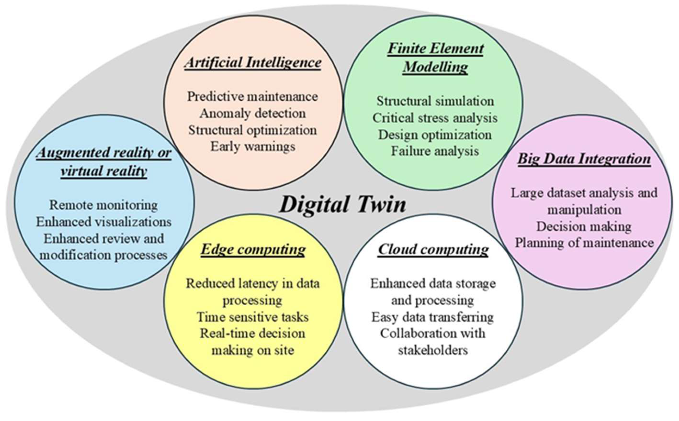
Figure 2.
The DT of a bridge based on FE modelling.
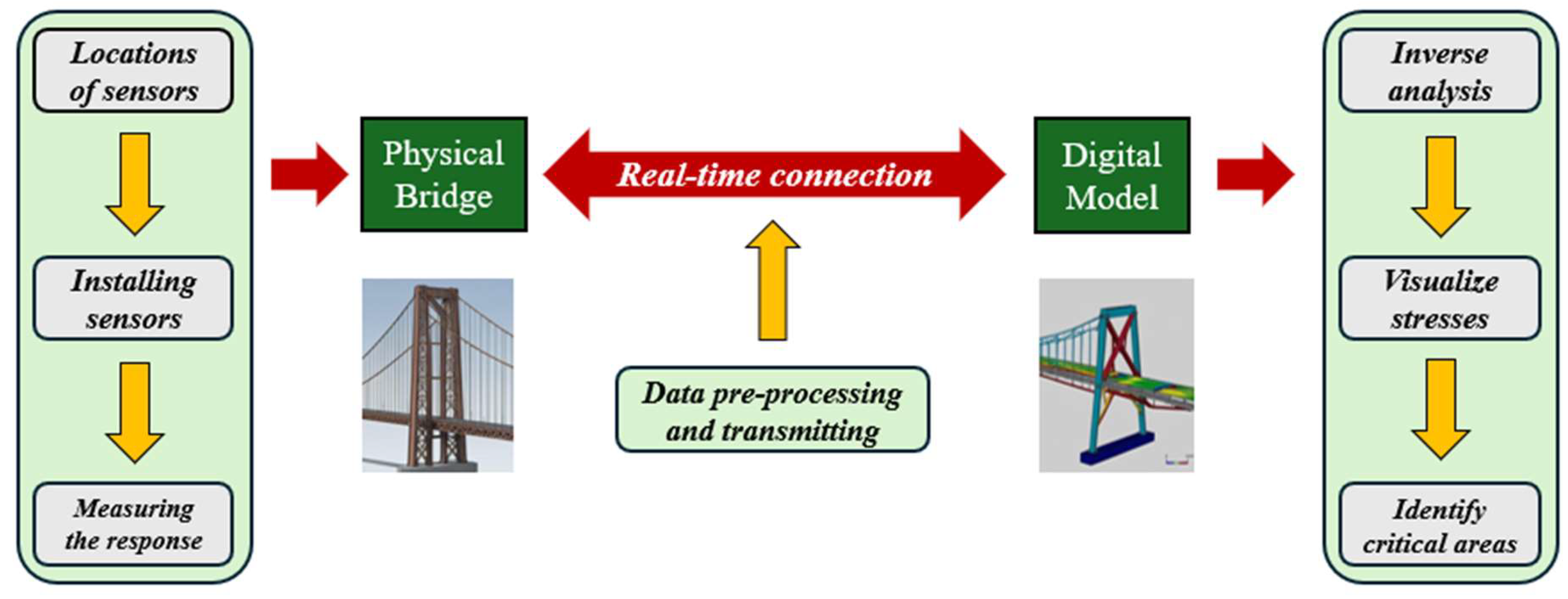
Figure 3.
The schematic of the methodology.
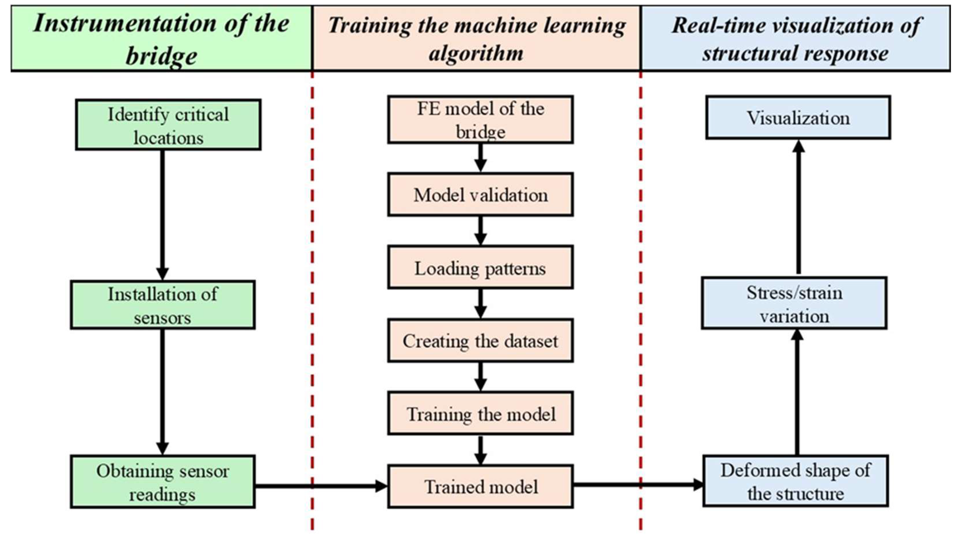
Figure 4.
Experimental laboratory-scale bridge.
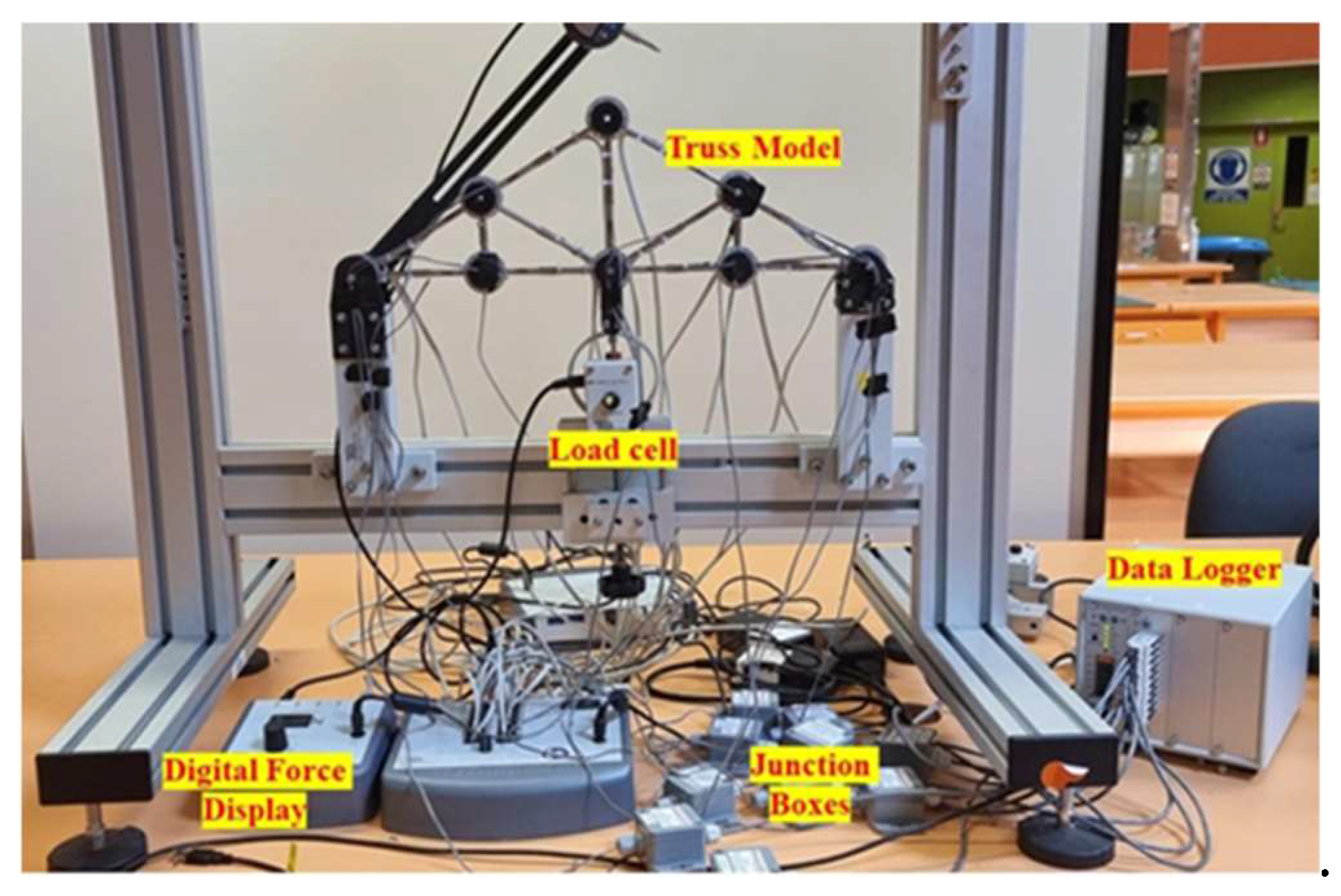
Figure 5.
Configuration of sensors.
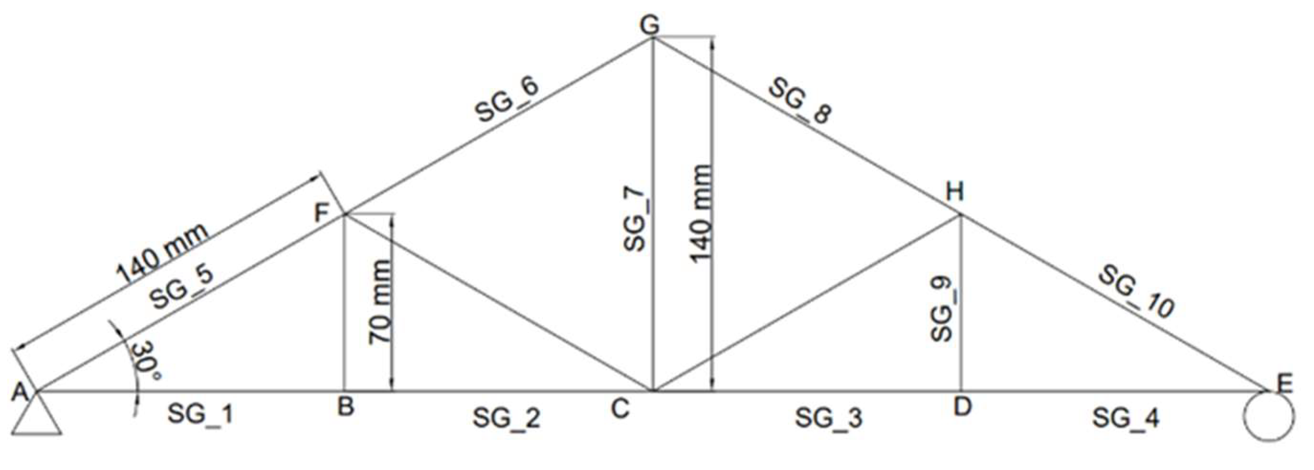
Figure 6.
Validated FE model of the bridge for zero loads.
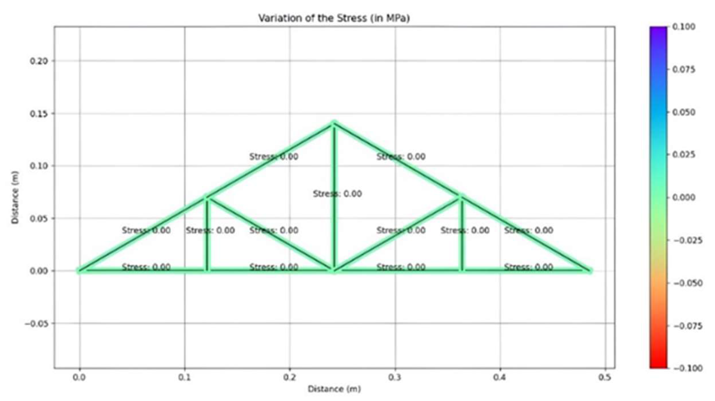
Figure 7.
Distribution of input and output data.
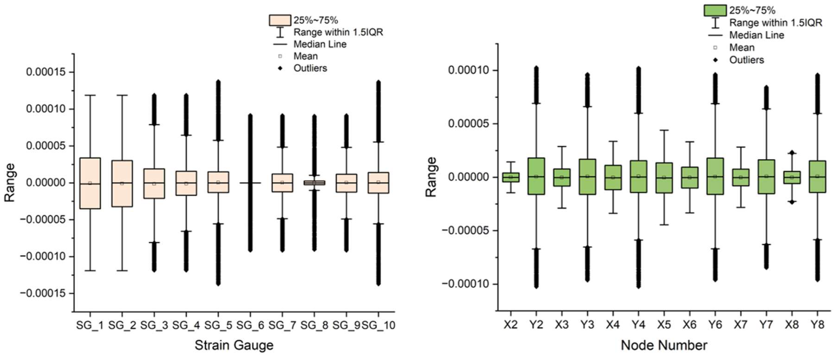
Figure 8.
First two levels of one decision tree of the developed model.
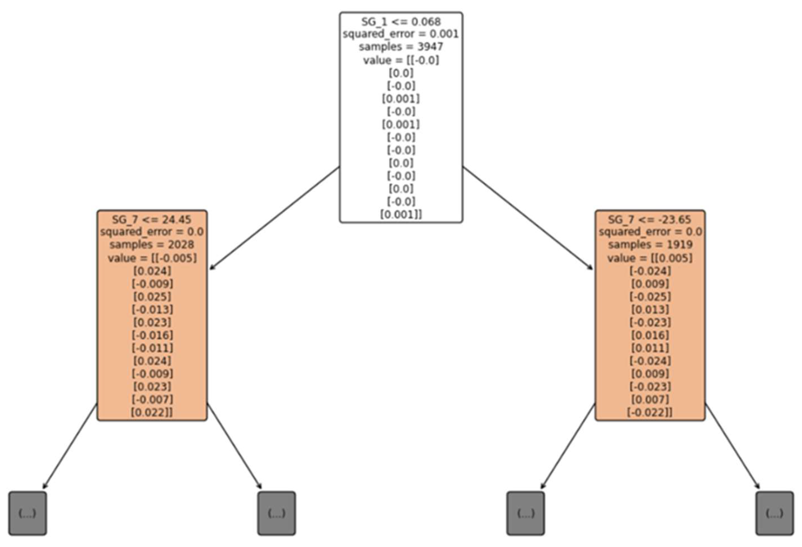
Figure 9.
First few stages of one decision tree of the developed XGBoost model.
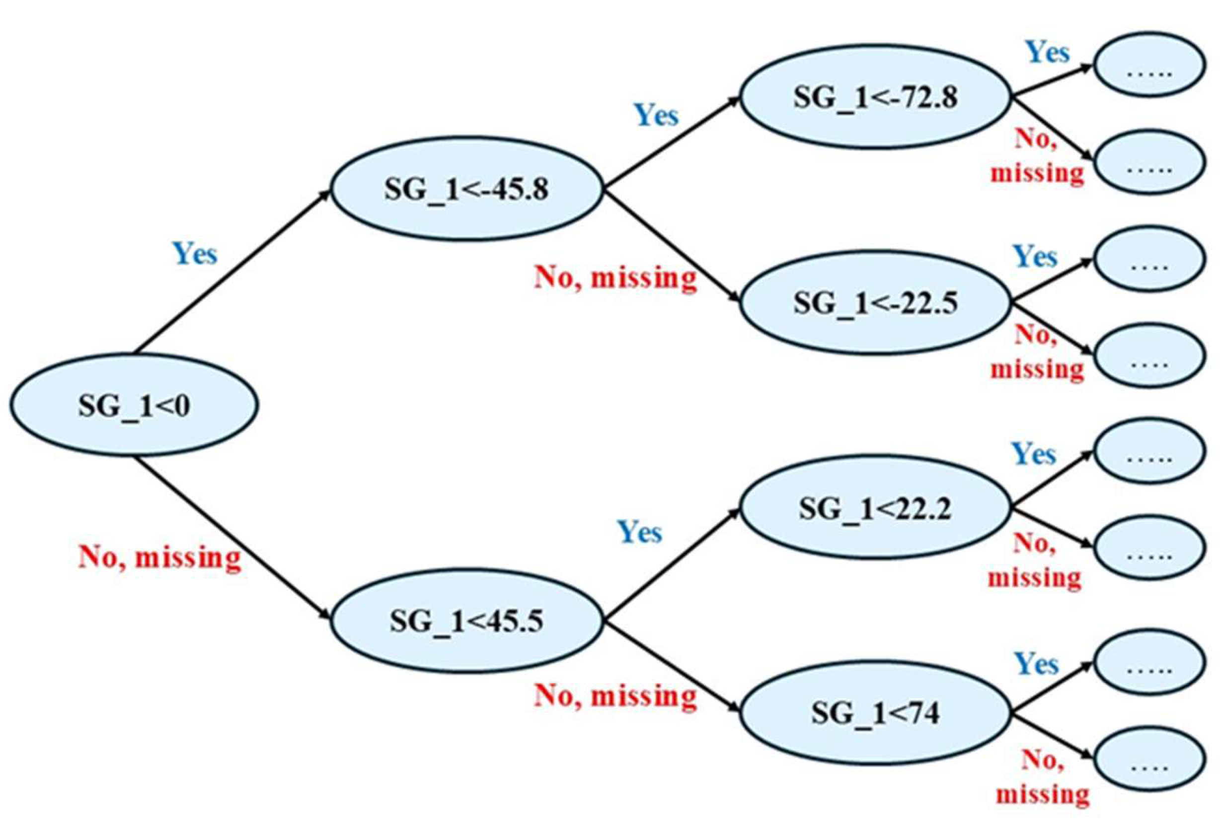
Figure 10.
The schematic of the developed MLP model.
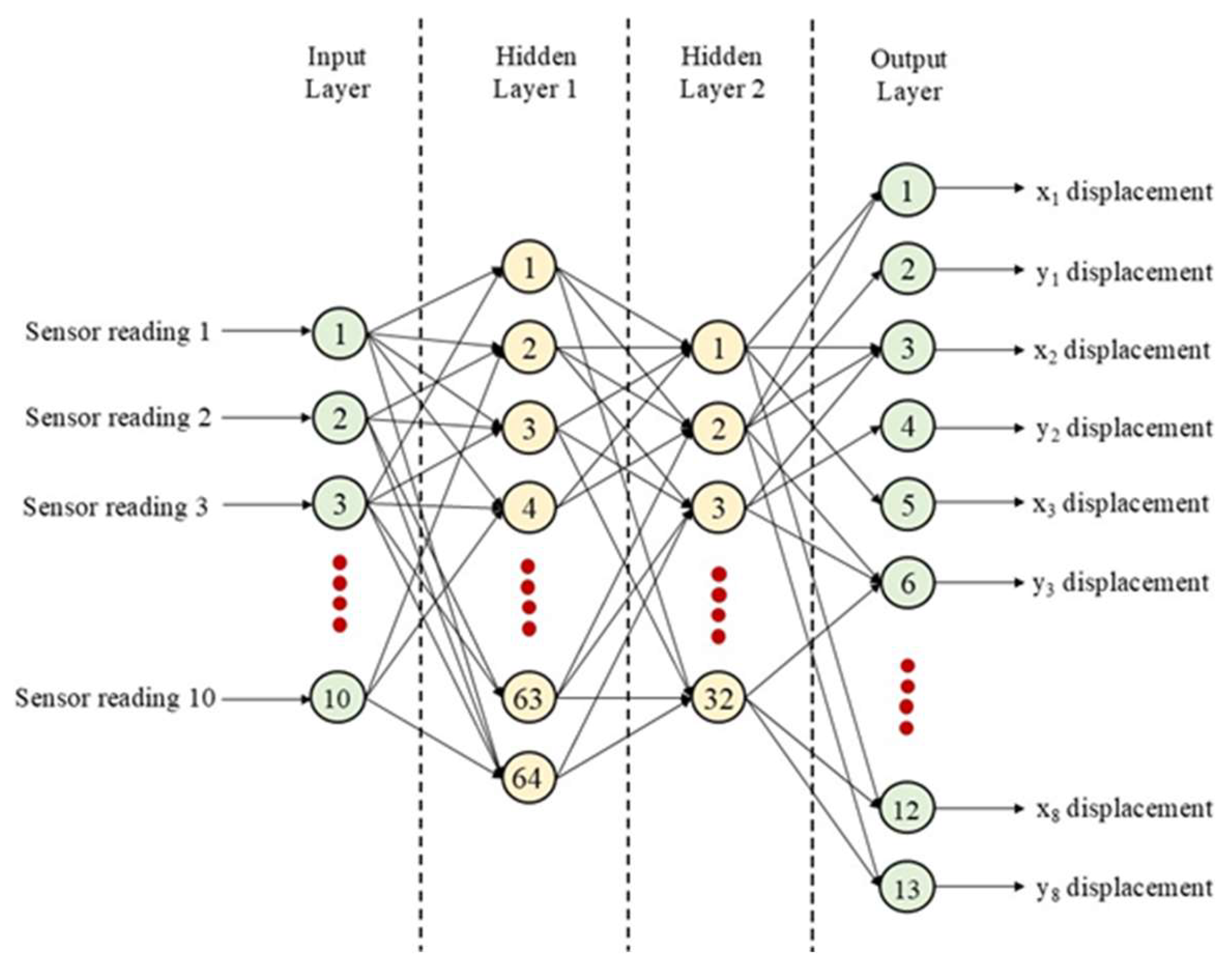
Figure 11.
RMSE values of 5 folds.
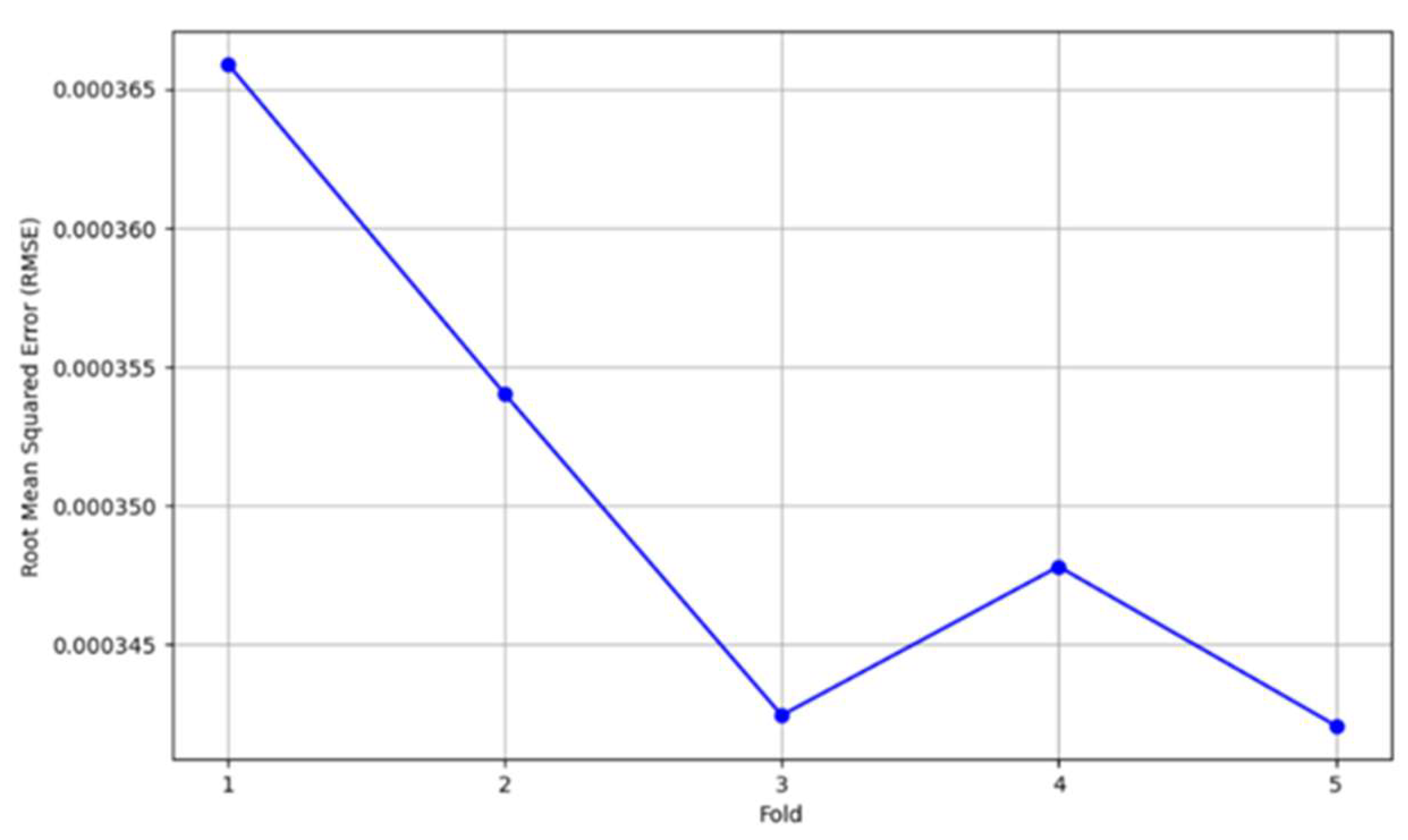
Figure 12.
Comparison of the predicted and actual data.
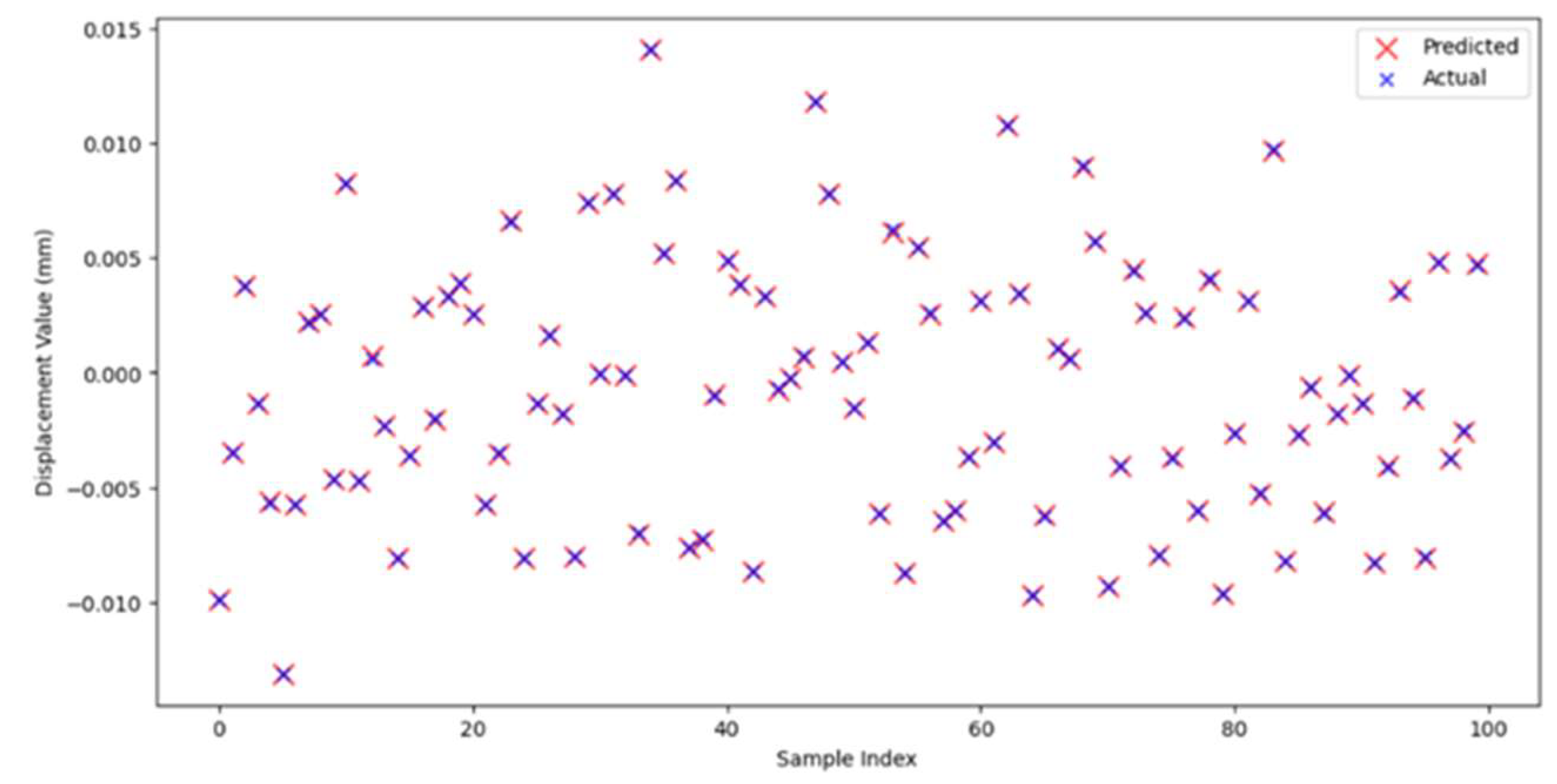
Figure 13.
Variation of the error with iterations.
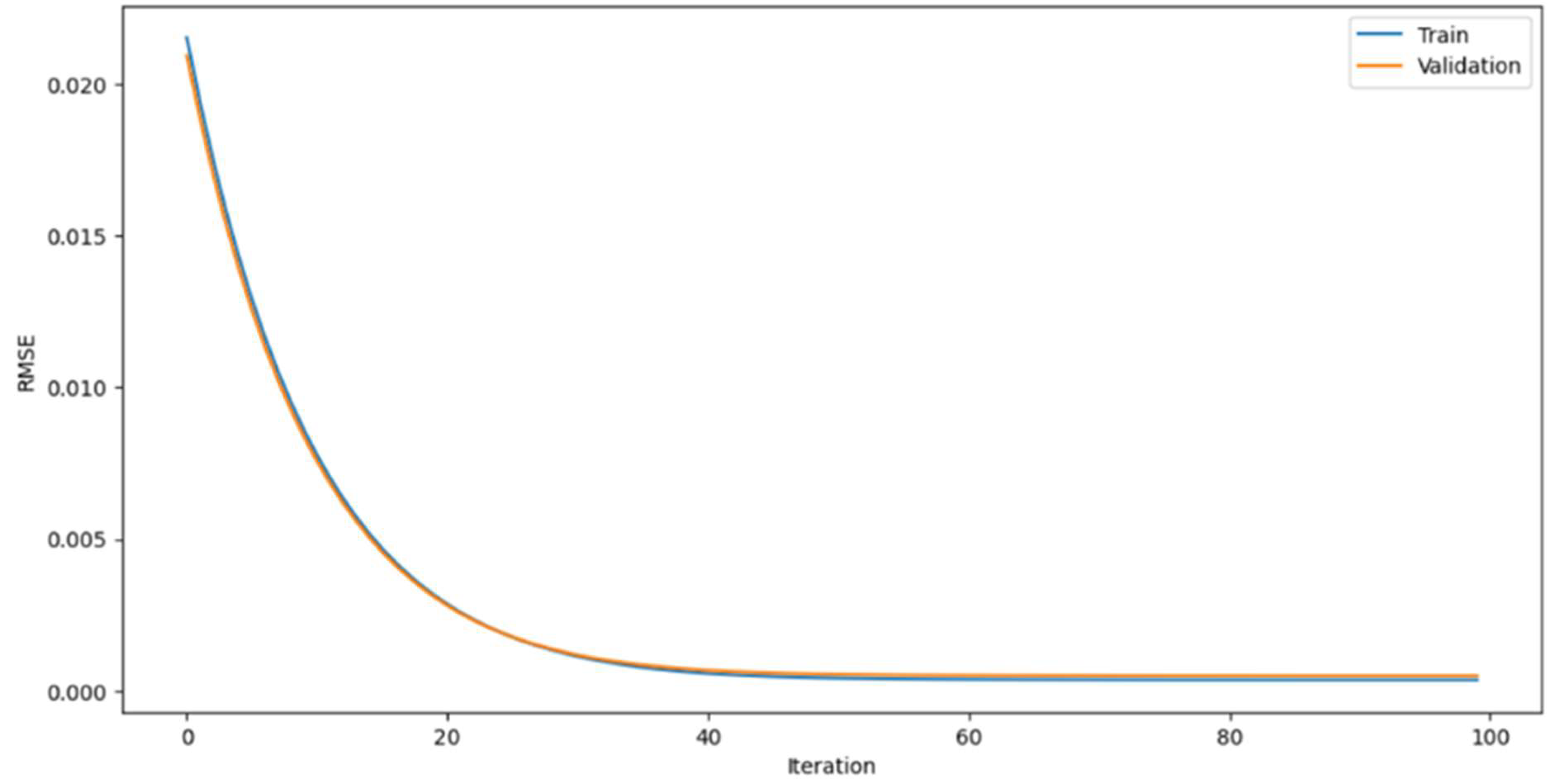
Figure 14.
Comparison of the predicted and actual data.
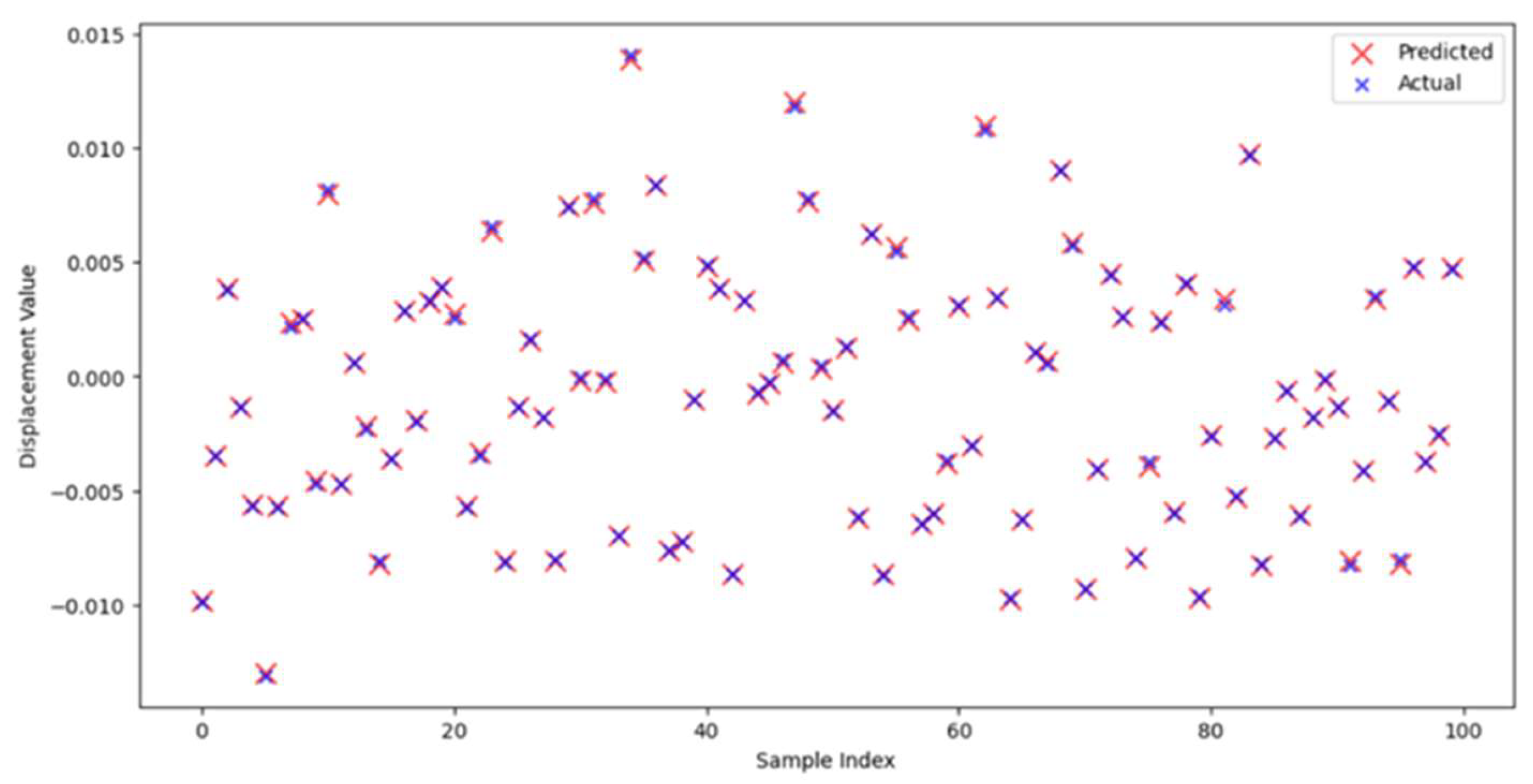
Figure 15.
Variation of the error with iterations.
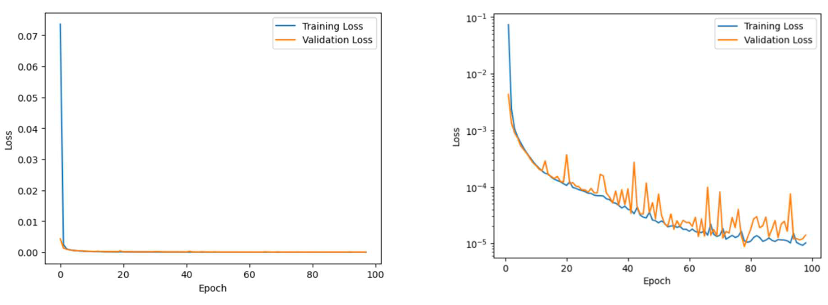
Figure 16.
Comparison of the predicted and actual data.
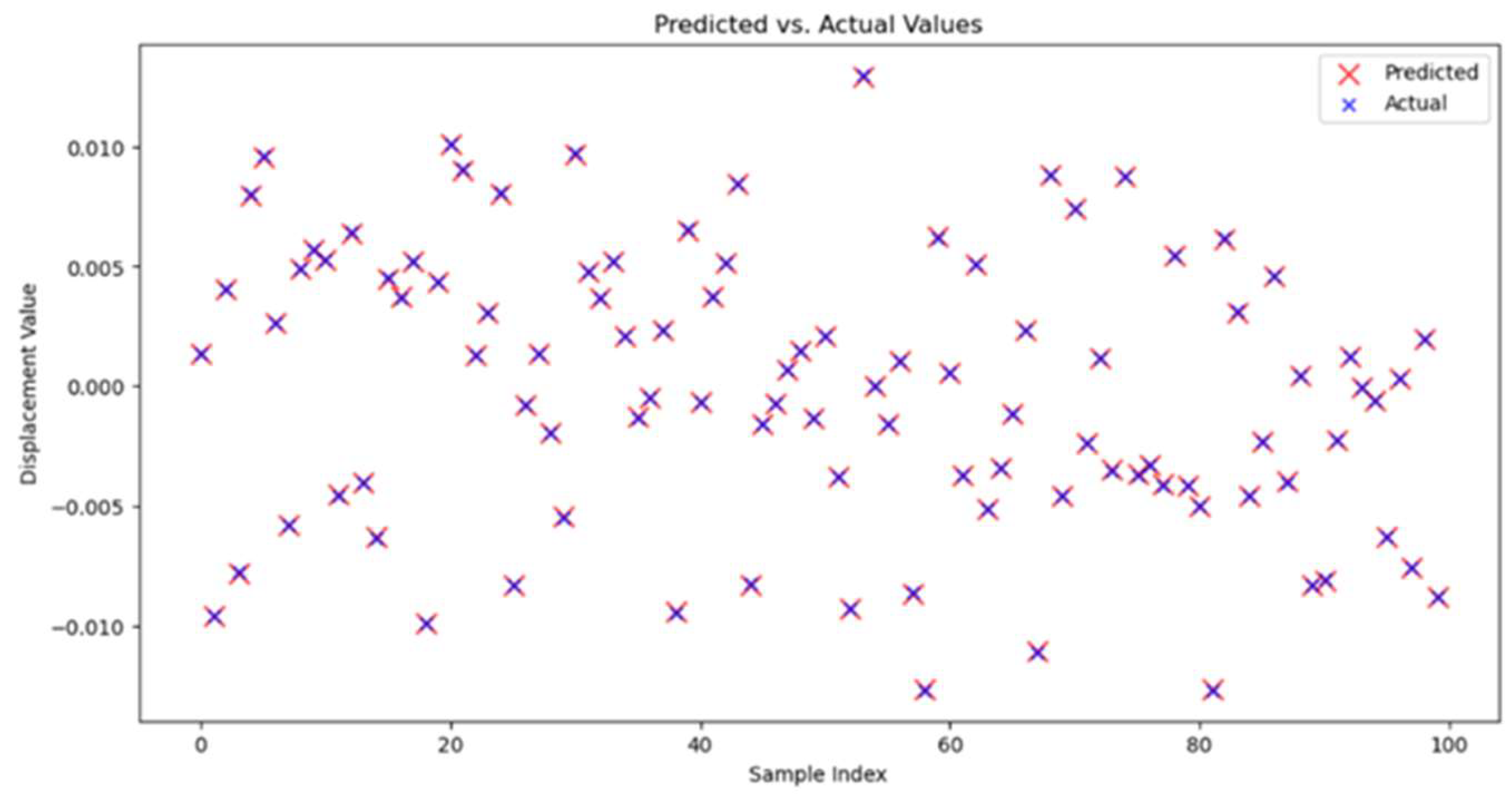
Figure 17.
Variation of the RMSE value with the size of the dataset.
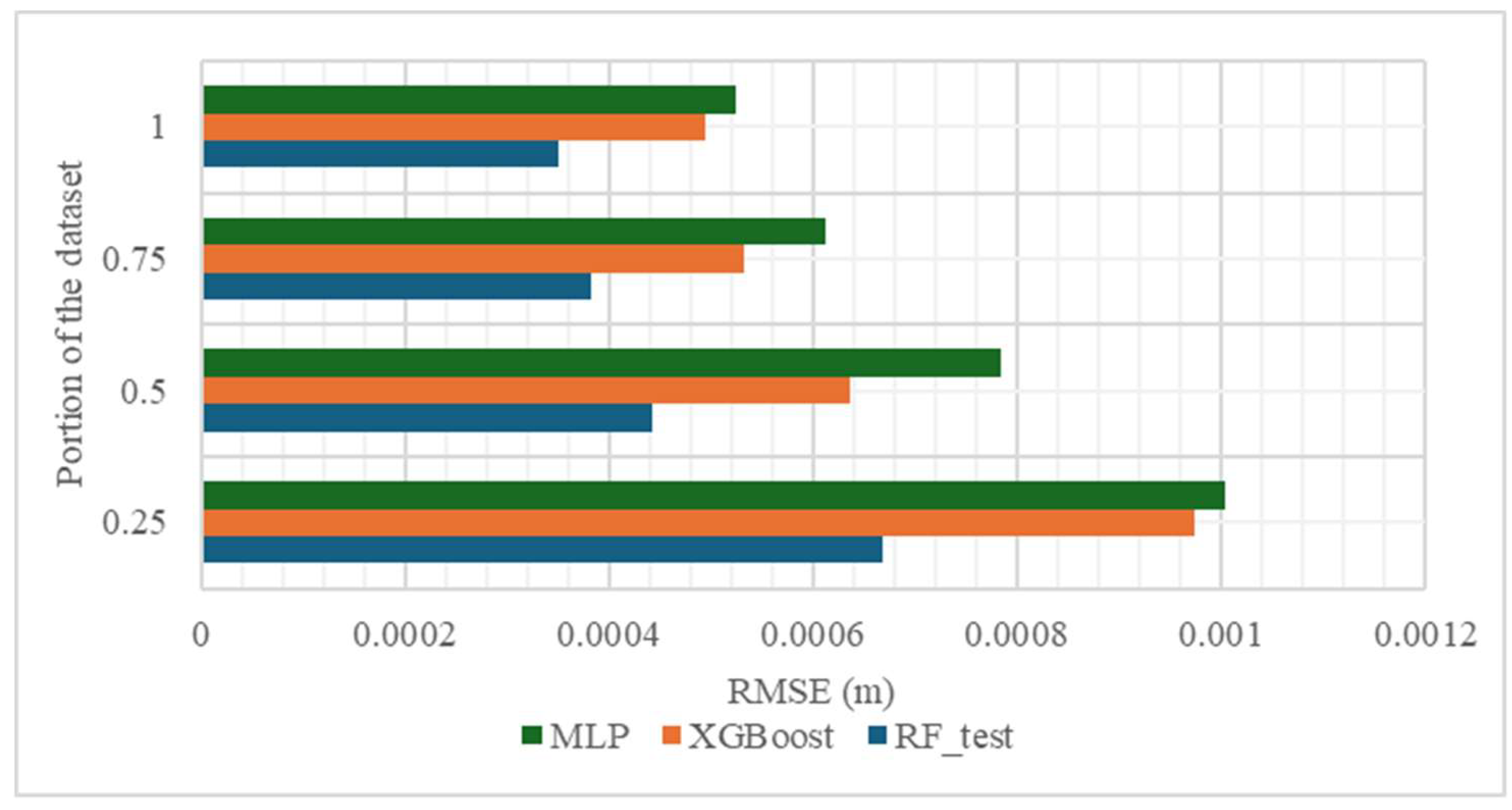
Figure 18.
Variation of the RMSE value with the size of the dataset.


Table 1.
Comparison of RMSE values and training time.
| Model Type | Test RMSE (mm) | Validation RMSE (mm) | Training time (s) |
|---|---|---|---|
| RF model | 0.000350 | 0.000341 | 13.60 |
| XGBoosting algorithm | 0.000494 | 0.000507 | 1.10 |
| MLP algorithm | 0.000524 | 0.000535 | 20.99 |
Table 2.
Inference times of each model.
| Model Architecture | Inference time (s) |
|---|---|
| RF model | 0.005 |
| XGBoost | 0.001 |
| MLP | 0.044 |
Disclaimer/Publisher’s Note: The statements, opinions and data contained in all publications are solely those of the individual author(s) and contributor(s) and not of MDPI and/or the editor(s). MDPI and/or the editor(s) disclaim responsibility for any injury to people or property resulting from any ideas, methods, instructions or products referred to in the content. |
© 2024 by the authors. Licensee MDPI, Basel, Switzerland. This article is an open access article distributed under the terms and conditions of the Creative Commons Attribution (CC BY) license (http://creativecommons.org/licenses/by/4.0/).
Copyright: This open access article is published under a Creative Commons CC BY 4.0 license, which permit the free download, distribution, and reuse, provided that the author and preprint are cited in any reuse.


