
Submitted:
13 November 2024
Posted:
14 November 2024
You are already at the latest version
Abstract
This study presents a novel end-to-end architecture based on edge detection for autonomous driving. The architecture has been designed to bridge the domain gap between synthetic and real-world images for end-to-end autonomous driving applications and includes custom edge detection layers before the Efficient Net convolutional module. To train the architecture, RGB and depth images were used together with inertial data as inputs to predict the driving speed and steering wheel angle. To pretrain the architecture, a synthetic multimodal dataset for autonomous driving applications was created. The dataset includes driving data from 100 diverse weather and traffic scenarios, gathered from multiple sensors including cameras and an IMU as well as vehicle control variables. The results show that including edge detection layers in the architecture improves performance for transfer learning when using synthetic and real-world data. In addition, pretraining with synthetic data reduces training time and enhances model performance when using real-world data.
Keywords:
end-to-end architectures
; multimodal synthetic dataset
; autonomous driving
1. Introduction
End-to-end neural networks are evolving rapidly in artificial intelligence and have become particularly popular in the field of autonomous driving. Traditional autonomous driving systems are modular in nature, where the driving problem is divided into subtasks operating independently, such as object detection [1,2], localization [3], trajectory planning [4], and control [5]. While this approach allows for specialized task optimization, it also introduces significant drawbacks, particularly in terms of error propagation between modules and computational inefficiencies [6]. The end-to-end approach, also known as direct perception, offers substantial benefits, such as reduced complexity [7], decreased error propagation [8], and improved computational efficiency [9], making it an appealing solution for autonomous driving applications.
End-to-end architectures learn driving related behaviors, resulting in more integrated and efficient autonomous driving systems [10]. These architectures enable the mapping of raw sensor inputs from the perception system directly to control commands for autonomously driving a vehicle. Different approaches to solving the end-to-end problem exist, while most studies focus on generating outputs directly, others incorporate intermediate steps such as trajectory planning. For example, in [11] the authors addressed autonomous navigation by predicting future waypoints, using a front-facing RGB camera and maps, as an intermediate step between the input and control output. Other studies combine trajectory planning with direct perception, as seen in research using the Carla simulator. In the work by Wu et al. [12] the authors use an architecture with two branches: one branch predicts the trajectory, while the other focuses on the control variables. The trajectory branch uses encoder data to guide the control predictions, and the outputs from both branches are then fused.
In addition to different architectural approaches, the use of multimodal inputs is another key factor for improving the accuracy and robustness of end-to-end models [13,14]. By combining data from multiple sensors, such as cameras, IMU, LiDAR, and radar, these models can achieve a more comprehensive understanding of the environment. For instance, the TransFuser [15] architecture is based on transformers and fuses image and LiDAR data using self-attention layers. In this architecture, multiple transformer modules operate at different resolutions to merge features from the input data, which are then fed into a waypoint prediction architecture.
Expanding on the advantages of multimodal inputs, the choice of specific data types, such as RGB images and depth maps, has also been shown to significantly enhance the performance of end-to-end architectures, particularly those utilizing convolutional layers for feature extraction [16]. RGB images provide detailed visual information about the driving environment, while depth maps offer crucial spatial and distance data, helping to interpret the three-dimensional structure of the scene [17]. By fusing RGB images with depth maps, architectures can better perceive and navigate complex environments, as demonstrated by the work of Xiao et al. [18].
Synthetic data has gained popularity as a valuable resource for end-to-end applications, primarily due to the challenges of collecting high-quality real-world data. One of the main advantages of synthetic data is the ability to generate large datasets for training purposes. Although synthetic data can be a powerful tool, end-to-end architectures trained exclusively in simulated environments struggle to perform well in real-world scenarios without adaptation [19]. Transfer learning allows models initially trained in simulations to be fine-tuned using real-world data, helping bridge the gap between the two domains and enhancing the versatility of architectures across different environments and conditions. However, most current research on transfer learning focuses on specific tasks such as object detection [20,21] or reducing the domain gap [22,23], rather than extending to more complex applications like end-to-end driving systems, where models must directly output control commands for vehicles.
This work presents a state-of-the-art end-to-end architecture for autonomous driving based on the EfficientNetV2 architecture obtaining a high performance and efficiency. The architecture has been designed to bridge the domain gap between synthetic and real-world images for end-to-end autonomous driving applications and includes novel edge detection layers before the convolutional module for this purpose. The architecture is pretrained using a multimodal synthetic dataset: Carla Multimodal Raw Data (CarlaMRD), created using the Carla simulator. The pretrained architecture has then been fine-tuned for real world driving applications using the UPCT real-world dataset, obtaining promising results whilst reducing computation time.
2. Materials and Methods
2.1. Synthetic Dataset
The rapid advance in autonomous driving technology has increased the demand for high-quality datasets to train, validate, and test end-to-end architectures for predicting vehicle control variables. These datasets are crucial for the development of robust autonomous driving systems capable of navigating diverse and complex real-world scenarios. Traditionally, real-world datasets collected using sensor-equipped vehicles have been the foundation for developing these systems. However, collecting real-world data is very expensive and time-consuming, and it is often difficult to obtain large amounts of data for training purposes [24], causing interest in synthetic datasets as a viable alternative to increase in recent years [25].
Synthetic datasets contain artificially generated data that mimics the conditions and scenarios of real-world driving environments. These datasets are created using computer-generated imagery and physics-based simulations, offering a controlled environment where diverse driving situations can be systematically produced and manipulated [26]. This capability addresses several limitations of real-world datasets, such as variations in weather and lighting conditions [27], complicated traffic situations [28], and the need for extensive data labelling [29].
The evaluation of current synthetic datasets for perception and vehicle control reveals notable limitations and areas for improvement. Most existing synthetic datasets have been designed for very specific applications and include only the necessary sensors and data for performing certain tasks such as odometry [30], object detection [31], or for specific weather conditions [32]. In Table 1, a summary of the most popular synthetic driving datasets is presented, including sample size, perception sensors and vehicle control data, and whether the dataset include raw data or processed data. The most significant multimodal datasets are included and although not recent, the Udacity dataset is included as it was considered one of the most complete multimodal datasets [33].
Despite the large number of existing studies, most autonomous driving datasets provide labelled data primarily for classification tasks, such as semantic segmentation, rather than raw sensor data [28,29,34,35,36,37]. This limitation restricts the development and evaluation of end-to-end perception models [38], which rely on raw sensor inputs to directly predict driving actions or scene understanding without intermediate steps like segmentation [39]. Moreover, the public datasets identified lacked crucial driving control variables, such as steering wheel angle, acceleration, and vehicle speed. These variables are essential for the effective training and performance of end-to-end architectures. It was also observed that many synthetic datasets have a small sample size, considering that one of the advantages of simulators is the possibility of generating large amounts of synthetic data [35,36,37].
In this work CarlaMRD dataset has been designed collecting raw data from various sensors in different weather and traffic scenarios and can be adapted for use in different types of applications. The synthetic dataset has been developed using the CARLA simulator. CARLA is an open-source simulator for autonomous driving research designed to support development, training, and validation of autonomous urban driving systems. The simulation platform provides different urban scenarios, with buildings, vehicles, pedestrians, etc. and supports flexible specification of sensor suites and environmental conditions [40].
2.1.1. Simulation Setup
Before running simulations in CARLA and recording data, it is important to correctly configure the simulation. First a map must be chosen or created from scratch. For this dataset, six predefined Carla worlds have been chosen (Figure 1):
- (a)
- Town01 is a small simple residential village.
- (b)
- Town02 is a simple town with a mixture of residential and commercial buildings.
- (c)
- Town03 is a medium sized urban map with junctions and a roundabout.
- (d)
- Town04 is a small mountain village with an infinite loop highway.
- (e)
- Town05 is a squared-grid town with cross junctions and a bridge. It has multiple lanes in each direction to perform lane changes.
- (f)
- Town10 is a larger urban environment with skyscrapers and residential buildings.
The weather and time of day can also be modified. This can be done by custom defining each weather variable or choosing from one of fourteen predefined settings. In this work, some custom weather conditions have been defined as well as using the predefined functions. The adjustable weather and time of day variables are the following: (a) cloudiness, (b) precipitation, (c) sun altitude angle, (d) sun azimuth angle, (e) precipitation de-posits, (f) wind intensity, (g) fog density and (h) wetness.
In addition to the geographical and meteorological variables of the simulation, the traffic conditions can also be defined. For each of the simulations, vehicles have been added to create realistic traffic scenarios. A wide range of vehicles can be added, from different car models to trucks and emergency vehicles. For the simulations, a black Ford Lincoln MKZ model vehicle has been chosen. Pedestrians and cyclists also play an important role in autonomous driving tasks and have been added to the simulations for increased realism.
To gather the data from the driving simulations, a range of perception sensors have been configured onboard the simulated vehicle. The simulated sensors in Carla can be configured with similar variables to real-world sensors, such as resolution and field of view (fov) for cameras, or range and number of channels for LIDAR sensors. To position the sensors onboard the vehicle, a Carla transform consisting of 3D coordinates is used, with origin in the centre of the vehicle. The RGB and depth cameras have been situated above the front windscreen for a frontal view, while the LiDAR and IMU sensors have been positioned on the middle of the roof of the vehicle. The RADAR sensor has been positioned on the front of the vehicle above the bumper. The sensors used and their configuration for recording data during the simulations are shown in Table 2.
2.1.2. Simulation Design
To create the dataset, 100 simulations have been run, each with a duration of six minutes driving time, with the vehicle set to autopilot mode. The advantage of using lots of short simulations is that a larger variety of scenes can be recorded, combining different weather conditions and traffic situations. The vehicle is randomly spawned to one of the spawn points on the maps and is driven around the simulation scene, recording data from the sensors and vehicle control. To ensure accurate data synchronization and a precise temporal sequence, timestamp values have been recorded with the data for each sensor. Figure 2 shows some examples of the images captured by the RGB camera.
The data collected from each of the 100 simulations is saved to a directory. Inside this folder, the RGB and depth images are each saved in their respective directories. The data collected from the sensors (IMU, RADAR, LIDAR and vehicle control) is saved to an individual text file in csv format for each sensor.
Once all the of the simulations have been run, the data is reviewed to make sure that all the files have been saved correctly and that the simulation finished without any incidents. The timestamps from each of the different sensors are synchronised by the simulator, therefore for each sensor a data sample exists for that timestamp, without the need for manual synchronisation which is the case when using real-world data [41].
2.2. End-to-End Architecture Design
End-to-end architectures have played a significant role in the advance of deep learning, especially in the field of computer vision. In recent years, architectures containing convolutional layers have become the preferred architecture for tasks such as image classification, object detection, and segmentation due to their ability to extract meaningful patterns from visual data.
End-to-end architectures consist of a sequence of specialized layers that work together to transform the input data to obtain the desired results, in this case the control actions of the vehicle. These layers include convolutional layers which apply filters to detect local patterns in the image data, dense fully-connected layers which use the features extracted to make the final predictions and pooling layers which are commonly used to reduce the spatial dimensions of the data while preserving key features [9]. Additionally, custom layers can be used for applying specific functions to the input data. In end-to-end architectures, these layers are usually stacked multiple times, to deepen the ability of the network to extract increasingly complex features. To introduce non-linearity to the architecture and reduce vanishing gradient issues, non-linear activations like ReLU (Rectified Linear Unit), are commonly used in CNNs.
The end-to-end architecture proposed in this work is based on the EfficientNetV2B0 model, designed and implemented to efficiently handle both visual and inertial input data. This dual input structure is based on the architecture designed in the work by Navarro et al. [9], which found that incorporating additional input data improved results substantially. The model incorporates edge detection layers along with an EfficientNetV2B0 backbone, which is responsible for feature extraction from RGB and depth images. Additionally, the architecture includes dense layers specifically designed to process data from an Inertial Measurement Unit (IMU), integrating multiple sensor modalities.
The EfficientNetV2 architecture belongs to a family of models that range from B0, optimized for smaller images, to B3, suited for larger images. This family of models has consistently outperformed traditional CNNs, whilst at the same time offering an improved computational speed and efficiency in terms of parameters [42]. The EfficientNetV2 models are particularly noted for their ability to achieve better performance on smaller datasets compared to Vision Transformer models, which typically require larger datasets to achieve the best results models [43]. For example, the EfficientNetV2B0 model comprises 7.4 million parameters, significantly fewer than some Vision Transformer models, which can contain up to 304 million parameters. Furthermore, Vision Transformer models demand over 24 times more training time compared to the EfficientNetV2B0 architecture [42], making the latter a more practical choice for many applications, particularly when computational resources are limited. Another advantage of the EfficientNetV2 architectures is their flexibility in training. They can either be trained from scratch or leverage pre-trained weights from large datasets like ImageNet.
The EfficientNetV2B0 model was adapted and trained from scratch in this work, this was necessary due to the inclusion of depth images as an additional channel alongside the standard RGB input, resulting in four-channel images. The pre-trained ImageNet weights, designed for three-channel RGB images, were therefore incompatible with this extended input structure.
In the proposed architecture, the EfficientNetV2B0 model has been further modified to support dual input data, enabling the integration of additional sensor information such as linear acceleration, angular velocity, vehicle orientation, or even GPS data. While RGB and depth images serve as the primary inputs, IMU sensor data, specifically angular velocity, is utilized as a secondary input. This multi-modal input capability enhances the model’s ability to process and interpret complex environments. Additional output layers have also been incorporated into the architecture, increasing the total number of parameters to 7.67 million. An illustration of the architecture is provided in Figure 3, demonstrating how the different data streams are integrated into the CNN.
Before the images are fed into the EfficientNetV2B0 architecture, they undergo a series of pre-processing steps designed to enhance critical features using edge detection. This process is implemented through four Lambda layers, which emphasize areas in the image where significant intensity changes occur, typically marking object boundaries. These edge features help the model focus on important visual cues that are essential for driving-related tasks, such as identifying lanes, detecting obstacles, and recognizing nearby vehicles. By extracting these edges, the model becomes better equipped to concentrate on the most relevant aspects of the scene, improving its accuracy in interpreting complex driving environments.
The first two Lambda layers in the pre-processing pipeline handle basic input extraction, separating the RGB channels and the depth channel from the input image. The third Lambda layer applies edge detection specifically to the RGB channels using the Sobel operator, a widely used method for highlighting areas of rapid intensity change. The result is a set of edge maps that highlight key boundaries in the image. The fourth Lambda layer then normalizes the edge maps, ensuring consistent scaling and contrast for the model’s input. To further prepare the data for the EfficientNetV2B0 block, a Rescaling layer is used to standardize the pixel values.
Once pre-processing is complete, the images are passed to the EfficientNetV2B0 block, which contains 240 layers. This architecture is composed of various types of layers, including convolutional layers, batch normalization layers, and specialized operations organized into blocks. The efficient design of these blocks enables the model to process the image data effectively while maintaining a balance between speed and accuracy.
In addition to the image input, the architecture also processes IMU data, which is handled separately using two Dense layers. These layers transform the IMU data, which includes angular velocity, into a format that can be integrated with the visual data. The outputs of the EfficientNetV2B0 block and the processed IMU data are then merged using a Concatenate layer, combining the visual and sensor inputs.
At the output stage, the architecture splits into two branches, each responsible for predicting one of the output variables. These branches predict vehicle speed (Km/h) and steering angle (radians). Each branch consists of three Dense layers, followed by a final Dense layer with a size of one, corresponding to the single value predicted for each output variable. This branching design allows the model to make independent predictions for both vehicle speed and steering angle, leveraging the combined information from the RGB images, depth images, and IMU data to deliver accurate outputs. In the study performed by Navarro et al. [9], it was found that using a branch for each output variable obtained better results than using one vector output.
3. Results
3.1. Model Configuration
The end-to-end architecture has been used to validate the synthetic CarlaMRD dataset. The architecture has been designed and implemented using the Tensorflow 2.10 and Keras 2.10 libraries. The models have been trained on a PC with an NVIDIA GeForce RTX 3070 GPU. To train the model, 150850 samples from the synthetic dataset were used. 120x160 RGB and depth images, angular velocity in °/s from the IMU, and the vehicle control parameters, speed in km/h, and steering angle in radians. The hyperparameters applied are shown in Table 3. The RMSprop optimization function [44]
To avoid overfitting during training of the models, a stop condition which considers the validation metrics has been used. A patience of 10 epochs is used, after which if the model is no longer learning, training is stopped and the weights from the best epoch are restored. This method ensures that the model has finished training without overfitting occurring.
To split the data the K-Fold cross method has been used. The dataset has been split into six equal sets of 25141 samples, with five for training and testing each of the five folds, and one for validation. As a result, five models have been obtained, validated using the same set of validation data to obtain consistent results. The five models have then been tested using the corresponding test set for each fold, this way predictions are obtained for a larger amount of data giving a better idea of the performance of the model.
Three metrics have been calculated to evaluate the performance of the models. These metrics have been chosen to get a thorough view of how the model behaves and allow the results to be compared with those presented by other authors in literature:
- The Mean Absolute Error (MAE) which is the average of the absolute differences between the predicted and actual values.
- The Mean Absolute Percentage Error (MAPE) which is calculated dividing the MAE by the range of the speed and angle data. The range is the difference between the maximum and minimum values of the variables to predict.
- The coefficient of determination, R2 was used to evaluate the quality of the results obtained by the model.
The results obtained from each of the five models are shown in Table 4.
To obtain a global view of the models and their accuracy, the metrics have been calculated for all the test predictions from each of the five models, obtaining a total of 125705 predictions. The models took on average 28778 s to train, with 64 epochs. The overall results are shown in Table 5.
The results show that the models achieve a lower percentage error for detecting the steering angle compared to the vehicle speed. This is logical as it is usually easier to relate geometrical features such as the road lines than spatial information to calculate the speed, especially as the model applies edge detection to the RGB images before the convolutional layers of the Efficient Net block. However, regarding the coefficient of determination, the model appears to make better predictions for the speed variable.
To study the quality of the predictions, box and whisker plots for the speed and angle errors are shown in Figure 4. The median error of the speed prediction is close to zero with a value of 0.081 Km/h, and half of the errors have a value between -0.567 and 0.903 Km/h. For the angle predictions, the median error is negative at -0.058°, with the first quartile at -0.238° and the third quartile at 0.062°. For both the speed and angle predictions the error predictions take on a Gaussian distribution.
3.2. Application of the Pretrained CNN for Training with a Real-World Dataset
3.2.1. Real-World Dataset
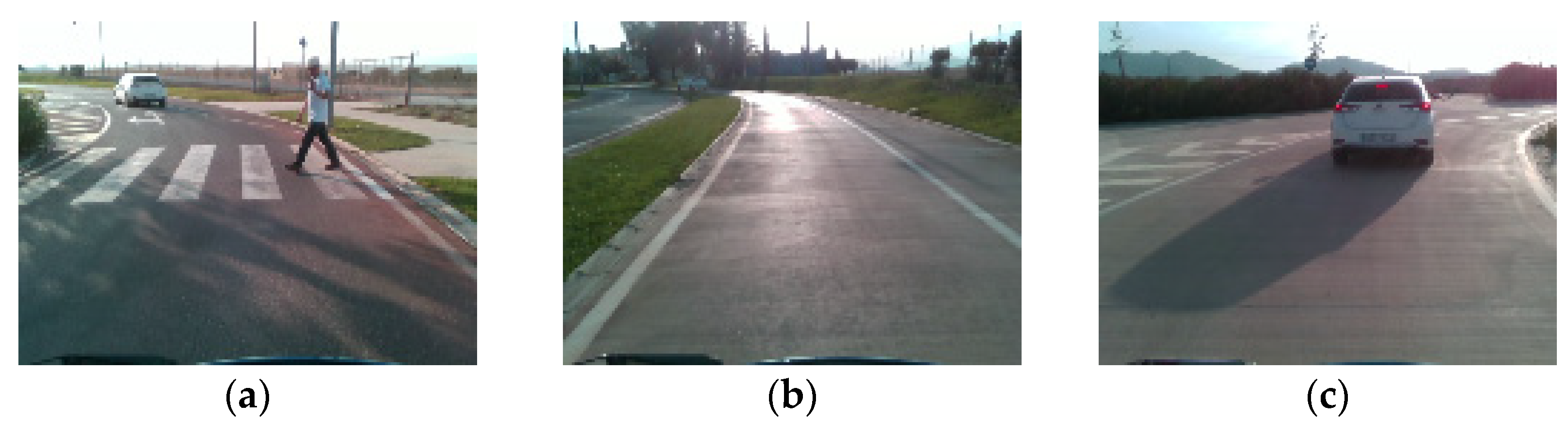
To study the usability of the synthetic dataset in real world applications, the pretrained model has been tested with a real driving dataset. For this application, the UPCT dataset containing real world driving data has been chosen [24]. The UPCT dataset is a public dataset which contains multimodal data from a variety of perception sensors including 3D LiDAR, RGB and depth cameras, IMU, GPS, encoders, as well as biometric data from the drivers. The data was recorded with state-of-the-art equipment onboard the UPCT’s CICar autonomous vehicle. The UPCT dataset contains 78000 samples which were obtained by a group of 30 different drivers performing tests along an urban route in southern Spain with real traffic, including roundabouts, junctions, merging traffic situations and street parking. The tests were performed at different times of day, including morning, afternoon and early evening.
Figure 5.
Example images from the UPCT dataset. (a) Pedestrian crossing; (b) saturation due to reflections on the road; (c) car braking [24].
Figure 5.
Example images from the UPCT dataset. (a) Pedestrian crossing; (b) saturation due to reflections on the road; (c) car braking [24].
3.2.2. Baseline Training with Only Real-World Data
First, the CNN model from Section 2.3 was trained using only the UPCT dataset to verify the performance of the model using real world data. The data was split into six equal groups of 13000 data samples, where five were used for training and testing with the K-fold method. The last group was used for validation for each of the five models in K-fold, to obtain consistent results and to have more data samples for testing. The results from testing each fold are shown in Table 6.
The metrics have been calculated for all the predictions from each of the five models, obtaining a total of 65000 predictions. The models took on average 19880 s to train, with 62 epochs. The results are shown in Table 7.
The results obtained by the models for predicting the vehicle speed using the real-world dataset are promising and have improved compared to those achieved with the synthetic dataset. The angle predictions, however, did not gain a significant improvement. As with the synthetic dataset, the angle predictions achieved a lower percentage error compared to the speed predictions.
Box and whisker plots for the speed and angle errors are shown in Figure 6. For the speed prediction errors, the median is close to zero with a value of -0.009 Km/h, and the first and third quartile values were of -0.315 Km/h and 0.290 Km/h, respectively. As shown by the box and whisker plots, the errors for both the speed and angle predictions the take on a Gaussian distribution with the median in the centre of the box. The median for the angle prediction errors is positive in this case with a value of 0.107°. The first and third quartile values were between -0.124° and -0.355°, respectively.
3.2.3. Pretraining with the Synthetic Dataset
The third test consisted in performing transfer learning using the synthetic dataset to pretrain the model, with the aim of reducing training time when training with real-world data. After training the models with the synthetic data, the weights from the Efficient Net convolutional blocks were saved and loaded to the model before training with the real dataset. The results obtained from transfer learning are shown in Table 8.
The metrics have been calculated for all predictions from the test sets each of the five models, obtaining a total of 65000 predictions. The models took on average 17350 s to train, with 56 epochs. The overall results are shown in Table 9.
From the results it can be observed that pretraining the model with a synthetic dataset and using the weights to train real data decreases the training time needed to obtain the same results. In this work the models needed on average six epochs less for training with the same real-world dataset compared to training with no previous information. Box and whisker plots of the prediction error values are shown in Figure 7.
The prediction errors calculated with the pretrained models are very similar to those with no pretraining once again with a Gaussian distribution with narrow boxes centred around the median value. The speed prediction errors a median of -0.040 Km/h was obtained, and quartile values between -0.461 Km/h and 0.376 Km/h. The median value of the angle prediction errors in this case is negative, with a value of -0.037° and the first and third quartiles with values of -0.306° and 0.217°, respectively.
3.3. Analysis of the Architecture with and Without Edge Detection Layers for Transfer Learning
Finally, the EdgeNet architecture was tested removing the edge detection layers from the architecture, to study the impact that these layers have on the performance of the architecture for transfer learning applications. The tests were repeated using the same datasets divided into five folds with the same training, validation and test sets, the same hyperparameters and stopping condition were used. Table 10 shows the results obtained by the architecture both with and without the edge detection block for both the synthetic and real-world datasets, as well as pretraining the architecture with the synthetic dataset to be used with real-world data.
It can be observed that when using the synthetic and real-world datasets alone, the architecture achieves a high performance with and without the edge detection block. However, the edge detection block proves to enhance the performance of the architecture significantly when pretraining with synthetic data. The edge detection block reduces the domain gap between the synthetic data and real-world data scenarios and with the pretrained weights a similar performance is achieved using real-world data with a lower computational cost than training from scratch. In the case of the speed prediction, with the edge detection layers the MAPE is reduced to almost a third compared to the architecture without edge detection layers. Box and whisker plots of the MAE error values for the transfer learning predictions without the edge detection block are shown in Figure 8.
The box and whisker plots for the architecture without edge detection layers (Figure 8) have a normal distribution similar to that of the architecture with edge detection layers (Figure 7). It can be observed that the interquartile range (IQR) of the MAE error values for the architecture without the edge detection block is greater for the prediction of both the speed and the angle variables. In the case of the speed MAE errors, without the edge detection block the errors have a significantly larger dispersion. Table 11 includes the numerical values of the median, quartile and IQR values of the MAE errors of the architectures with and without the edge detection block.
4. Discussion
The results obtained by the EdgeNet architecture were compared to those presented by other authors in literature. Several studies exist, mainly using real world ad-hoc datasets obtained or modified by the authors. Some authors used synthetic datasets and real-world datasets for training their architectures [45,46]. However, these were conducted as separate experiments, and the synthetic data was not used for pretraining the models. Table 10 shows a comparison of the results obtained in this work with other experiments using CNN models for end-to-end driving and details the type of dataset used and the variables predicted.

Table 12.
Comparison of the proposed model with the metrics of other End-to-end models.
| Authors, Ref. | Dataset | Data Type | Input | Output | MAE (km/h)/ (°) | MAPE (%) | R2 |
|---|---|---|---|---|---|---|---|
| Bojarski et al., [45,47] | Udacity | Synthetic | RGB | Steering Angle | 4.26 | - | - |
| Yang et al., [45] | Udacity | Synthetic | RGB | Speed/ Steering Angle | 0.68 / 1.26 | - | - |
| SAIC | Real | RGB | Speed | 1.62 | - | - | |
| Xu et al., [48] | BDDV | Real | RGB | Steering Angle | - | 15.4 | - |
| Wang et al., [46] | GAC | Real | RGB | Speed/Steering Angle | 4.25 / 3.55 | - | - |
| GTAV | Synthetic | RGB | Speed/Steering Angle | 3.28 / 2.84 | - | - | |
| Navarro et al., [9] | UPCT | Real | RGB + IMU | Speed/Steering Angle | 0.98 / 3.61 | 1.69 / 0.43 | - |
| Prasad [49] | - | Real | RGB | Steering Angle | - | - | 0.819 |
| Proposed: BorderNet | Carla | Synthetic | RGBD + IMU | Speed/Steering Angle | 1.47 / 0.51 | 1.59 / 0.55 | 0.977 / 0.948 |
| UPCT | Real World | RGBD + IMU | Speed/Steering Angle | 0.61 / 0.41 | 1.04 / 0.53 | 0.989 / 0.973 |
One of the first end-to-end deep neural network applications for autonomous driving was resented by Bojarski et al., [47]. They used the PilotNet model for object detection and steering angle prediction from just RGB image inputs from the Udacity dataset. The work by Yang et al. [45] built on these results and used the PilotNet to predict both vehicle speed and steering angle from the same Udacity RGB images. Xu et al. tested six different CNN models, some using LSTM architectures, to predict steering angle using 21000 short 36 s videos of RGB frames as training data. They used the real world BDDV dataset, and the best accuracy was obtained with a temporal CNN with an accuracy of 84.6 % [48]. In the work presented by Wang et al. [46], different end-to-end deep convolutional neural networks were tested to predict the speed and steering angle using RGB images as the input. It is worth noting that a better performance was obtained using the model with the synthetic dataset compared to using the real-world data. The authors in [9] completed a thorough study of three types of CNN with different inputs, one with RGB images, a second complementing the RGB images with IMU data and a third model using sequences of RGB images. The best results were achieved using the RGB images with an additional input of IMU data obtaining a MAPE of 1.69 % for the speed calculation and a MAPE of 0.43 % for predicting the steering wheel angle. The experiment conducted by Prasad et al. [49] presented an end-to-end CNN model to predict the steering angle from real-world RGB images on a small vehicle, the only metric given was the R2 score with a value of 0.819.
The end-to-end model presented in this work obtained a 99.30 % accuracy for speed calculation and a 99.49 % accuracy for predicting the steering angle, with the real-world dataset without pretrained weights. When using the model with the pretrained weights from training with the synthetic dataset, the model obtained a 98.95 % accuracy predicting speed and a 99.47 % accuracy predicting the steering angle with the real-world dataset. In addition, results show that by pretraining a CNN model with synthetic data, training time can be significantly reduced.
5. Conclusions
End-to-end architectures trained and tested using only simulated driving data have shown promising results. However, few approaches have focused on addressing the gap between simulation and reality, and the benefits that transfer learning applications have to offer. In this work, an end-to-end architecture has been developed, which not only has obtained a high performance with simulated data and real-world data alone but has also shown significant potential when used for transfer learning. To overcome the differences between simulated and real-world images, edge detection layers were introduced into the architecture before the EfficientNetV2 module. These layers extract crucial edge information before the convolutional module, helping to bridge the domain gap between synthetic and real-world data. The architecture was evaluated using two datasets: a simulated dataset generated by the Carla simulator and the real-world UPCT dataset.
The proposed architecture integrates both RGB and depth images as inputs, along with a second input branch for inertial data, to enhance accuracy and performance. The architecture was trained and tested in three scenarios: (1) with the CarlaMRD synthetic dataset, (2) with the real-world UPCT dataset, and (3) with the UPCT dataset using the pretrained weights from the synthetic dataset. The results obtained with the architecture including the edge detection block were then compared to those obtained by the same architecture without the edge detection. It was proven that the inclusion of edge detection layers significantly improved the predictions for the speed variable when using an architecture pretrained with synthetic data.
The results show that pretraining with the synthetic dataset significantly reduces training time using weights pretrained with synthetic data when training with real-world data. Furthermore, the architecture obtained a high performance and computational efficiency in predicting vehicle control variables, whether pretraining was used or not. The results achieved demonstrate a notable improvement compared to similar studies conducted by other authors, highlighting the effectiveness and robustness of the proposed architecture.
Author Contributions
Conceptualization, L.M., P.J.N., and F.R; methodology, L.M., P.J.N.; software, L.M.; validation, P.J.N. and F.R.; formal analysis, P.J.N.; investigation, L.M.; resources, P.J.N.; data curation, L.M.; writing—original draft preparation, L.M.; writing—review and editing, P.J.N., F.R and L.M; visualization, P.J.N.; supervision, F.R.; project administration, P.J.N.; funding acquisition, P.J.N. All authors have read and agreed to the published version of the manuscript.
Funding
This work was partially supported by AEI METROPOLIS (ref. PLEC2021-007609) Spanish Government projects.
Data Availability Statement
The dataset presented is available on the Zenodo platform: https://zenodo.org/uploads/11193178
Conflicts of Interest
The authors declare no conflicts of interest.
References
- Navarro, P. J.; Fernández, C.; Borraz, R.; Alonso, D. A Machine Learning Approach to Pedestrian Detection for Autonomous Vehicles Using High-Definition 3D Range Data. Sensors 2017, 17.
- Ros García, A.; Miller, L.; Fernández, C.; Navarro, P. J. Obstacle Detection using a Time of Flight Range Camera. In 2018 IEEE International Conference on Vehicular Electronics and Safety (ICVES); 2018; pp. 1–6.
- Akai, N.; Morales, L. Y.; Yamaguchi, T.; Takeuchi, E.; Yoshihara, Y.; Okuda, H.; Suzuki, T.; Ninomiya, Y. Autonomous driving based on accurate localization using multilayer LiDAR and dead reckoning. In 2017 IEEE 20th International Conference on Intelligent Transportation Systems (ITSC); 2017; pp. 1–6.
- Teng, S.; Hu, X.; Deng, P.; Li, B.; Li, Y.; Ai, Y.; Yang, D.; Li, L.; Xuanyuan, Z.; Zhu, F.; Chen, L. Motion Planning for Autonomous Driving: The State of the Art and Future Perspectives. IEEE Transactions on Intelligent Vehicles 2023, 8, 3692–3711.
- Borraz, R.; Navarro, P. J.; Fernández, C.; Alcover, P. M. Cloud Incubator Car: A Reliable Platform for Autonomous Driving. Applied Sciences 2018, 8.
- Kong, J.; Pfeiffer, M.; Schildbach, G.; Borrelli, F. Kinematic and dynamic vehicle models for autonomous driving control design. In 2015 IEEE Intelligent Vehicles Symposium (IV); 2015; pp. 1094–1099.
- Wu, P.; Jia, X.; Chen, L.; Yan, J.; Li, H.; Qiao, Y. Trajectory-guided Control Prediction for End-to-end Autonomous Driving: A Simple yet Strong Baseline. In Advances in Neural Information Processing Systems; 2022; pp. 6119–6132.
- Chitta, K.; Prakash, A.; Geiger, A. NEAT: Neural Attention Fields for End-to-End Autonomous Driving. In Proceedings of the IEEE/CVF International Conference on Computer Vision (ICCV); 2021; pp. 15793–15803.
- Navarro, P. J.; Miller, L.; Rosique, F.; Fernández-Isla, C.; Gila-Navarro, A. End-to-End Deep Neural Network Architectures for Speed and Steering Wheel Angle Prediction in Autonomous Driving. Electronics (Switzerland) 2021, 10.
- Mozaffari, S.; Al-Jarrah, O. Y.; Dianati, M.; Jennings, P.; Mouzakitis, A. Deep Learning-Based Vehicle Behavior Prediction for Autonomous Driving Applications: A Review. IEEE Transactions on Intelligent Transportation Systems 2022, 23, 33–47.
- Xu, J.; Wu, T. End-to-end autonomous driving based on image plane waypoint prediction. In 2022 International Symposium on Control Engineering and Robotics (ISCER); 2022; pp. 132–137.
- Wu, P.; Jia, X.; Chen, L.; Yan, J.; Li, H.; Qiao, Y. Trajectory-guided Control Prediction for End-to-end Autonomous Driving: A Simple yet Strong Baseline. In Advances in Neural Information Processing Systems; 2022; pp. 6119–6132.
- Cai, P.; Wang, S.; Wang, H.; Liu, M. Carl-Lead: Lidar-based End-to-End Autonomous Driving with Contrastive Deep Reinforcement Learning. 2021, 2109.08473.
- Shao, H.; Wang, L.; Chen, R.; Li, H.; Liu, Y. Safety-Enhanced Autonomous Driving Using Interpretable Sensor Fusion Transformer. In Proceedings of The 6th Conference on Robot Learning; 2023; pp. 726–737.
- Chitta, K.; Prakash, A.; Jaeger, B.; Yu, Z.; Renz, K.; Geiger, A. TransFuser: Imitation With Transformer-Based Sensor Fusion for Autonomous Driving. IEEE Trans Pattern Anal Mach Intell 2023, 45, 12878–12895.
- Chen, D.; Krahenbuhl, P. Learning From All Vehicles. In Proceedings of the IEEE/CVF Conference on Computer Vision and Pattern Recognition (CVPR); 2022; pp. 17222–17231.
- Li, W.; Gu, J.; Dong, Y.; Dong, Y.; Han, J. Indoor scene understanding via RGB-D image segmentation employing depth-based CNN and CRFs. Multimed Tools Appl 2019, 79, 35475–35489.
- Xiao, Y.; Codevilla, F.; Gurram, A.; Urfalioglu, O.; López, A. M. Multimodal End-to-End Autonomous Driving. IEEE Transactions on Intelligent Transportation Systems 2022, 23, 537–547.
- Chen, L.; Wu, P.; Chitta, K.; Jaeger, B.; Geiger, A.; Li, H. End-to-end Autonomous Driving: Challenges and Frontiers. IEEE Trans Pattern Anal Mach Intell 2024, 1–20.
- Chen, Y.; Rong, F.; Duggal, S.; Wang, S.; Yan, X.; Manivasagam, S.; Xue, S.; Yumer, E.; Urtasun, R. GeoSim: Realistic Video Simulation via Geometry-Aware Composition for Self-Driving. In Proceedings of the IEEE/CVF Conference on Computer Vision and Pattern Recognition (CVPR); 2021; pp. 7230–7240.
- Zhang, L.; Wen, T.; Min, J.; Wang, J.; Han, D.; Shi, J. Learning Object Placement by Inpainting for Compositional Data Augmentation. In {Computer Vision - ECCV 2020; 2020; pp. 566–581.
- Chen, Y.; Li, W.; Sakaridis, C.; Dai, D.; Van Gool, L. Domain Adaptive Faster R-CNN for Object Detection in the Wild. In Proceedings of the IEEE Conference on Computer Vision and Pattern Recognition (CVPR); 2018.
- Zhang, H.; Luo, G.; Tian, Y.; Wang, K.; He, H.; Wang, F.-Y. A Virtual-Real Interaction Approach to Object Instance Segmentation in Traffic Scenes. IEEE Transactions on Intelligent Transportation Systems 2021, 22, 863–875.
- Rosique, F.; Navarro, P. J.; Miller, L.; Salas, E. Autonomous Vehicle Dataset with Real Multi-Driver Scenes and Biometric Data. Sensors 2023, 23.
- Song, Z.; He, Z.; Li, X.; Ma, Q.; Ming, R.; Mao, Z.; Pei, H.; Peng, L.; Hu, J.; Yao, D.; Zhang, Y. Synthetic Datasets for Autonomous Driving: A Survey. IEEE Transactions on Intelligent Vehicles 2024, 9, 1847–1864.
- Paulin, G.; Ivasic-Kos, M. Review and analysis of synthetic dataset generation methods and techniques for application in computer vision. Artif Intell Rev 2023, 56, 9221–9265.
- Sakaridis, C.; Dai, D.; Van Gool, L. Semantic Foggy Scene Understanding with Synthetic Data. Int J Comput Vis 2018, 126, 973–992.
- Sun, T.; Segu, M.; Postels, J.; Wang, Y.; Van Gool, L.; Schiele, B.; Tombari, F.; Yu, F. SHIFT: A Synthetic Driving Dataset for Continuous Multi-Task Domain Adaptation. IEEE/CVF Conference on Computer Vision and Pattern Recognition (CVPR) 2022, 21371–21382.
- Alberti, E.; Tavera, A.; Masone, C.; Caputo, B. IDDA: A Large-Scale Multi-Domain Dataset for Autonomous Driving. IEEE Robot Autom Lett 2020, 5, 5526–5533.
- Kloukiniotis, A.; Papandreou, A.; Anagnostopoulos, C.; Lalos, A.; Kapsalas, P.; Nguyen, D-, V.; Moustakas, K. CarlaScenes: A synthetic dataset for odometry in autonomous driving. In IEEE Computer Society Conference on Computer Vision and Pattern Recognition Workshops; 2022; pp. 4519–4527.
- Ramesh, A. N.; Correas-Serrano, A. M. G.-H. SCaRL- A Synthetic Multi-Modal Dataset for Autonomous Driving. In International Conference on Microwaves for Intelligent Mobility; 2024.
- Pitropov, M.; Garcia, D. E.; Rebello, J.; Smart, M.; Wang, C.; Czarnecki, K.; Waslander, S. Canadian Adverse Driving Conditions dataset. Int J Rob Res 2020, 40, 681–690.
- Yin, H.; Berger, C. When to use what data set for your self-driving car algorithm: An overview of publicly available driving datasets. In IEEE 20th International Conference on Intelligent Transportation Systems (ITSC); 2017; pp. 1–8.
- Ros, G.; Sellart, L.; Materzynska, J.; Vazquez, D.; Lopez, A. M. The SYNTHIA Dataset: A Large Collection of Synthetic Images for Semantic Segmentation of Urban Scenes. In IEEE Conference on Computer Vision and Pattern Recognition (CVPR); 2016; pp. 3234–3243.
- Saleh, F. S.; Aliakbarian, M. S.; Salzmann, M.; Petersson, L.; Alvarez, J. M. Effective Use of Synthetic Data for Urban Scene Semantic Segmentation. In European Conference on Computer Vision (ECCV); 2018.
- Li, X.; Wang, K.; Tian, Y.; Yan, L.; Deng, F.; Wang, F.-Y. The ParallelEye Dataset: A Large Collection of Virtual Images for Traffic Vision Research. IEEE Transactions on Intelligent Transportation Systems 2019, 20, 2072–2084.
- Hurl, B.; Czarnecki, K.; Waslander, S. Precise Synthetic Image and LiDAR (PreSIL) Dataset for Autonomous Vehicle Perception. In IEEE Intelligent Vehicles Symposium (IV); 2019.
- Koopman, P.; Wagner, M. Challenges in Autonomous Vehicle Testing and Validation. SAE Int J Transp Saf 2016, 4, 15–24.
- Tampuu, A.; Matiisen, T.; Semikin, M.; Fishman, D.; Muhammad, N. A Survey of End-to-End Driving: Architectures and Training Methods. IEEE Trans Neural Netw Learn Syst 2022, 33, 1364–1384.
- Dosovitskiy, A.; Ros, G.; Codevilla, F.; Lopez, A.; Koltun, V. CARLA: An Open Urban Driving Simulator. In Proceedings of the 1st Annual Conference on Robot Learning; 2017; pp. 1–16.
- {Vitols, G.; Bumanis, N.; Arhipova, I.; Meirane, I. LiDAR and Camera Data for Smart Urban Traffic Monitoring: Challenges of Automated Data Capturing and Synchronization. In Applied Informatics; 2021; pp. 421–432.
- Tan, M.; Le, Q. V EfficientNetV2: Smaller Models and Faster Training. In INTERNATIONAL CONFERENCE ON MACHINE LEARNING, VOL 139; 2021; pp. 7102–7110.
- Dosovitskiy, A.; Beyer, L.; Kolesnikov, A.; Weissenborn, D.; Zhai, X.; Unterthiner, T.; Dehghan, M.; Minderer, M.; Heigold, G.; Gelly, S.; Uszkoreit, J.; Houlsby, N. AN IMAGE IS WORTH 16X16 WORDS: TRANSFORMERS FOR IMAGE RECOGNITION AT SCALE. In International Conference on Learning Representations; 2021.
- Masand, A.; Chauhan, S.; Jangid, M.; Kumar, R.; Roy, S. ScrapNet: An Efficient Approach to Trash Classification. IEEE Access 2021, 9, 130947–130958.
- Yang, Z.; Zhang, Y.; Yu, J.; Cai, J.; Luo, J. End-to-end Multi-Modal Multi-Task Vehicle Control for Self-Driving Cars with Visual Perceptions. In 24th International Conference on Pattern Recognition (ICPR); 2018; pp. 2289–2294.
- Wang, D.; Wen, J.; Wang, Y.; Huang, X.; Pei, F. End-to-End Self-Driving Using Deep Neural Networks with Multi-auxiliary Tasks. Automotive Innovation 2019, 2, 127–136.
- Bojarski, M.; Yeres, P.; Choromanska, A.; Choromanski, K.; Firner, B.; Jackel, L.; Muller, U. Explaining How a Deep Neural Network Trained withEnd-to-End Learning Steers a Car. In Computer Vision and Pattern Recognition (cs.CV); 2017.
- Xu, H.; Gao, Y.; Yu, F.; Darrell, T. End-To-End Learning of Driving Models From Large-Scale Video Datasets. In IEEE Conference on Computer Vision and Pattern Recognition (CVPR); 2017; pp. 2174–2182.
- Prasad Mygapula, D. V; Adarsh, S.; Sajith Variyar, V. V; Soman, K. P. CNN based End to End Learning Steering Angle Prediction for Autonomous Electric Vehicle. In Fourth International Conference on Electrical, Computer and Communication Technologies (ICECCT); 2021; pp. 1–6.
Figure 1.
Carla world maps. (a) Town01; (b) Town02; (c) Town03; (d) Town04; (e) Town05; (f) Town10.

Figure 2.
Example RGB images. (a) Town01: Wet Sunset; (b) Town02: Heavy rain noon; (c) Town03: Foggy afternoon; (d) Town04: Sunny afternoon; (e) Town05: Sunny noon; (f) Town10: Cloudy evening.
Figure 2.
Example RGB images. (a) Town01: Wet Sunset; (b) Town02: Heavy rain noon; (c) Town03: Foggy afternoon; (d) Town04: Sunny afternoon; (e) Town05: Sunny noon; (f) Town10: Cloudy evening.
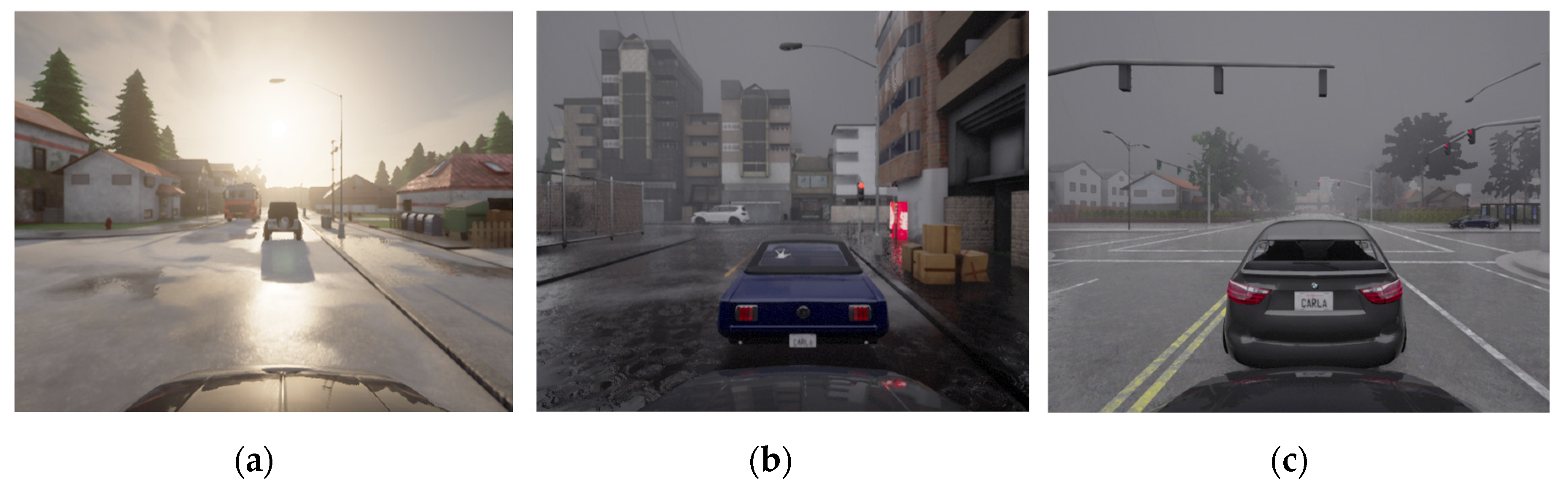
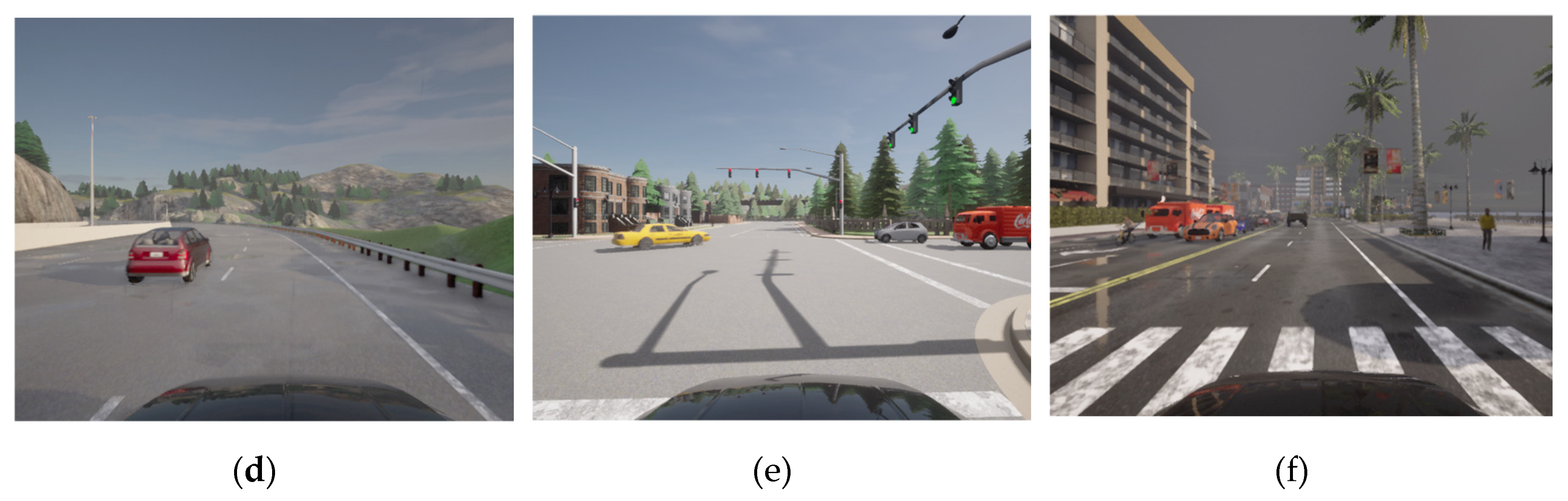
Figure 3.
End-to-end architecture with Efficient Net V2 B0 backbone.
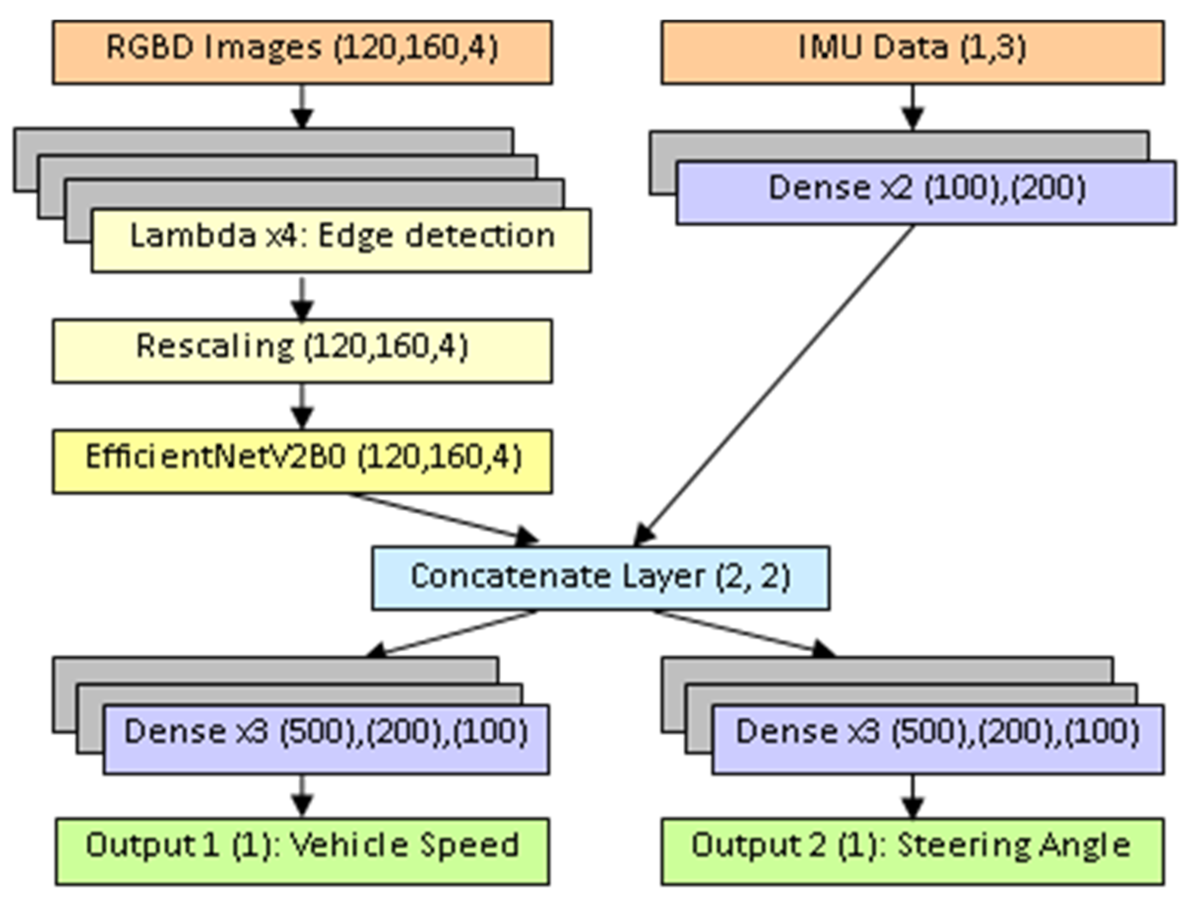
Figure 4.
Box and whisker plots for speed errors in Km/h (top) and angle errors in degrees (bottom).
Figure 4.
Box and whisker plots for speed errors in Km/h (top) and angle errors in degrees (bottom).
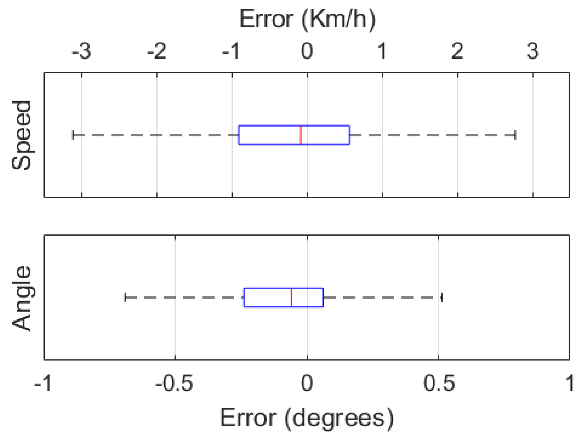
Figure 6.
Box and whisker plots for speed errors in Km/h (top) and angle errors in degrees (bottom).
Figure 6.
Box and whisker plots for speed errors in Km/h (top) and angle errors in degrees (bottom).
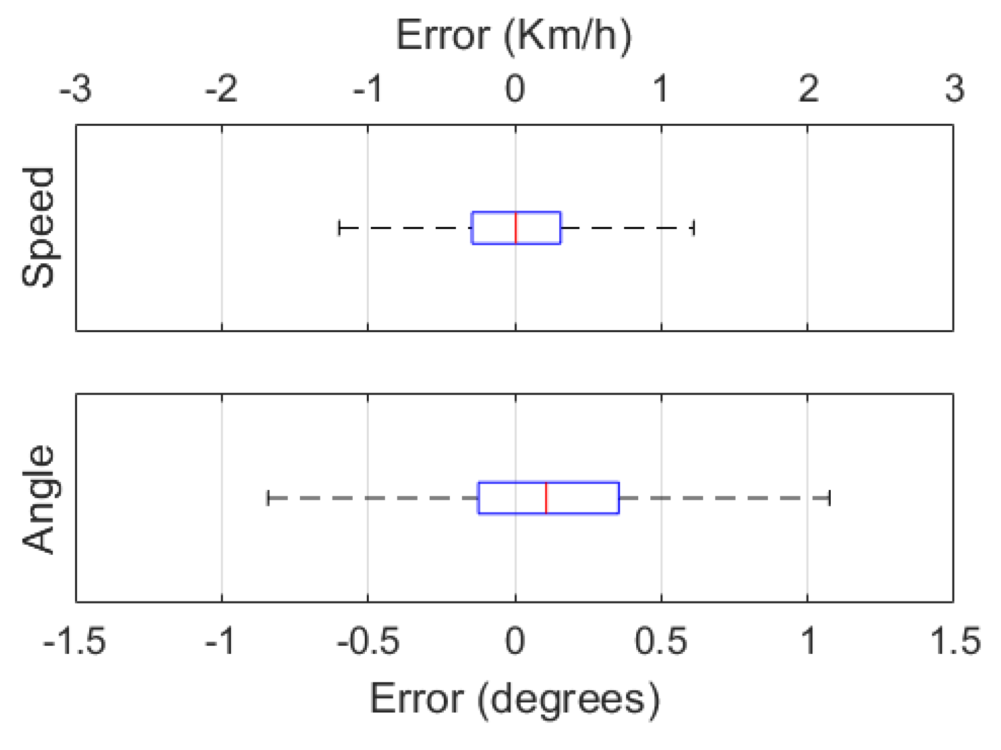
Figure 7.
Box and whisker plots for speed errors in Km/h (top) and angle errors in degrees (bottom).
Figure 7.
Box and whisker plots for speed errors in Km/h (top) and angle errors in degrees (bottom).
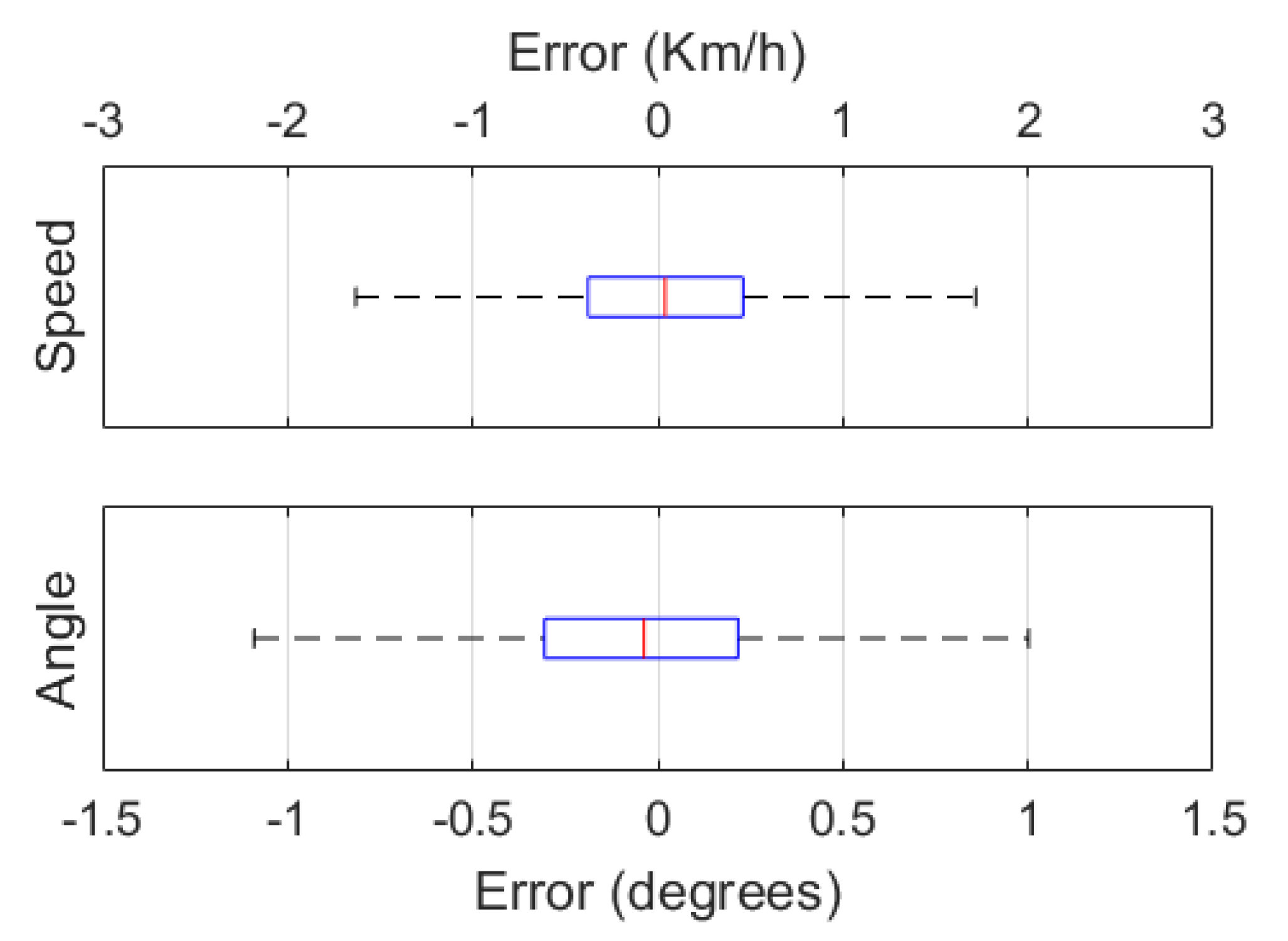
Figure 8.
Box and whisker plots for speed errors in Km/h (top) and angle errors in degrees (bottom).
Figure 8.
Box and whisker plots for speed errors in Km/h (top) and angle errors in degrees (bottom).
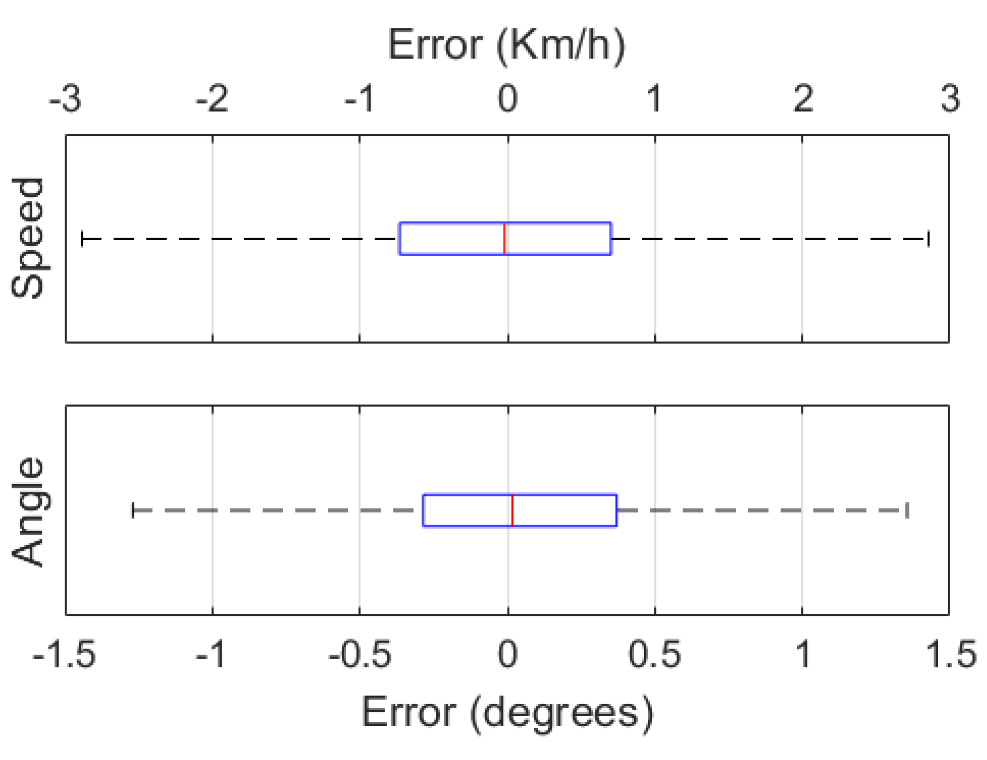
Table 1.
Synthetic datasets with sensors for perception, vehicle control variables and data type.
| Dataset/Year | Samples | Image Type | IMU | LIDAR | RADAR | Vehicle Control | Raw Data |
|---|---|---|---|---|---|---|---|
| Udacity [33]/2016 | 34 K | RGB | Yes | Yes | No | Yes | Yes |
| SYNTHIA [34]/2016 | 213K | RGB | No | No | No | No | No |
| VEIS [35]/2018 | 61K | RGB | No | No | No | No | No |
| ParallelEye [36]/2019 | 40 K | RGB | No | No | No | No | No |
| PreSIL 6[37]/2019 | 50 K | RGB | No | Yes | No | No | No |
| IDDA [29]/2020 | 1M | RGB, D | No | No | No | No | No |
| CarlaScenes [30]/2021 | - | RGB, D | Yes | Yes | No | No | Partial |
| SHIFT[28]/2022 | 2.6 M | RGB, D | Yes | No | No | No | No |
| Proposed: CarlaMRD | 150K | RGB, D | Yes | Yes | Yes | Yes | Yes |
Table 2.
Sensors used in the perception system and vehicle control variables.
| Sensor | Data Type |
|---|---|
| RGB Camera | RGB image 640x480, fov=90°. |
| Depth Camera | Depth image 640x480, fov=90°. |
| IMU |
Acceleration x,y,z (m/s2). Angular Velocity x,y,z (°/s). Orientation x,y,z (°). |
| LIDAR |
3D pointcloud, x,y,z,intensity. Channels=64, f=20, range=100m, points per second = 500000. |
| RADAR |
2D pointcloud: polar coordinates, distance and velocity. Horizontal fov=45°, Vertical fov=30°. |
| Vehicle Control |
Steering angle (rad). Speed (km/h). Accelerator pedal (Value from 0 to 1). Brake pedals (Value from 0 to 1). |
Table 3.
Configuration of hyperparameters.
| Parameter | Variable |
|---|---|
| Batch size | 20 |
| Optimization algorithm | RMSprop |
| Loss function | Huber |
| Metric | Mean Absolute Error |
| Learning rate | 0.001 |
Table 4.
MAE, MAPE and R2 obtained using the synthetic dataset.
| Fold | Variable | MAE (Km/h, °) | MAPE | R2 |
|---|---|---|---|---|
| 1 | Speed | 1.66 | 1.80 % | 0.973 |
| Angle | 0.65 | 0.71 % | 0.944 | |
| 2 | Speed | 1.21 | 1.32 % | 0.986 |
| Angle | 0.41 | 0.46 % | 0.952 | |
| 3 | Speed | 1.41 | 1.53 % | 0.978 |
| Angle | 0.45 | 0.50 % | 0.952 | |
| 4 | Speed | 1.80 | 1.95 % | 0.971 |
| Angle | 0.96 | 0.62 % | 0.939 | |
| 5 | Speed | 1.27 | 1.37 % | 0.981 |
| Angle | 0.45 | 0.49 % | 0.954 |
Table 5.
MAE, MAPE and R2 obtained by the models for the synthetic dataset.
| Variable | MAE (Km/h, °) | MAPE | R2 |
|---|---|---|---|
| Speed | 1.47 | 1.59 % | 0.978 |
| Angle | 0.51 | 0.55 % | 0.948 |
Table 6.
MAE, MAPE and R2 obtained using real world data.
| Fold | Variable | MAE (Km/h, °) | MAPE | R2 |
|---|---|---|---|---|
| 1 | Speed | 0.39 | 0.67 % | 0.996 |
| Angle | 0.34 | 0.44 % | 0.985 | |
| 2 | Speed | 0.48 | 0.82 % | 0.995 |
| Angle | 0.49 | 0.62 % | 0.953 | |
| 3 | Speed | 0.34 | 0.58 % | 0.997 |
| Angle | 0.34 | 0.44 % | 0.984 | |
| 4 | Speed | 0.44 | 0.75 % | 0.995 |
| Angle | 0.39 | 0.50 % | 0.969 | |
| 5 | Speed | 0.38 | 0.66 % | 0.996 |
| Angle | 0.40 | 0.51 % | 0.977 |
Table 7.
MAE, MAPE and R2 obtained with real world data.
| Variable | MAE (Km/h, °) | MAPE | R2 |
|---|---|---|---|
| Speed | 0.40 | 0.69 % | 0.996 |
| Angle | 0.39 | 0.50 % | 0.974 |
Table 8.
MAE, MAPE and R2 obtained using pretrained weights to train with real world data.
| Fold | Variable | MAE (Km/h, °) | MAPE | R2 |
|---|---|---|---|---|
| 1 | Speed | 0.68 | 1.17 % | 0.987 |
| Angle | 0.43 | 0.55 % | 0.969 | |
| 2 | Speed | 0.54 | 0.94 % | 0.992 |
| Angle | 0.36 | 0.47 % | 0.976 | |
| 3 | Speed | 0.52 | 0.90 % | 0.992 |
| Angle | 0.39 | 0.50 % | 0.978 | |
| 4 | Speed | 0.70 | 1.21 % | 0.987 |
| Angle | 0.50 | 0.64 % | 0.961 | |
| 5 | Speed | 0.58 | 0.99 % | 0.989 |
| Angle | 0.38 | 0.49 % | 0.981 |
Table 9.
MAE, MAPE and R2 obtained using pretrained weights to train with real world data.
| Variable | MAE (Km/h, °) | MAPE | R2 |
|---|---|---|---|
| Speed | 0.61 | 1.04 % | 0.989 |
| Angle | 0.41 | 0.53 % | 0.973 |
Table 10.
MAE, MAPE and R2 obtained by the architecture with and without the edge detection block.
| Dataset | Variable | MAE (Km/h, °) | MAPE | R2 | |||
|---|---|---|---|---|---|---|---|
| w edges | w/o edges | w edges | w/o edges | w edges | w/o edges | ||
| CarlaMRD | Speed | 1.47 | 0.40 | 1.59 % | 0.69 % | 0.978 | 0.996 |
| Angle | 0.50 | 0.39 | 0.55 % | 0.50 % | 0.948 | 0.974 | |
| UPCT | Speed | 0.40 | 0.39 | 0.69 % | 0.68 % | 0.996 | 0.995 |
| Angle | 0.39 | 0.39 | 0.50 % | 0.51 % | 0.974 | 0.972 | |
| UPCT pretrained | Speed | 0.60 | 1.66 | 1.04 % | 2.86 % | 0.989 | 0.911 |
| Angle | 0.41 | 0.60 | 0.52 % | 0.77 % | 0.973 | 0.929 | |
Table 11.
Median and quartile MAE values with and without the edge detection block.
| Dataset | Variable | Q1 | Q2 (Median) | Q3 | IQR | ||||
|---|---|---|---|---|---|---|---|---|---|
| w edges | w/o edges | w edges | w/o edges | w edges | w/o edges | w edges | w/o edges | ||
| UPCT pretrained | Speed (Km/h) | -0.461 | -0.703 | -0.040 | 0.019 | 0.375 | 0.731 | 0.836 | 1.434 |
| Angle (°) | -0.306 | -0.285 | -0.037 | 0.017 | 0.217 | 0.371 | 0.523 | 0.656 | |
Disclaimer/Publisher’s Note: The statements, opinions and data contained in all publications are solely those of the individual author(s) and contributor(s) and not of MDPI and/or the editor(s). MDPI and/or the editor(s) disclaim responsibility for any injury to people or property resulting from any ideas, methods, instructions or products referred to in the content. |
© 2024 by the authors. Licensee MDPI, Basel, Switzerland. This article is an open access article distributed under the terms and conditions of the Creative Commons Attribution (CC BY) license (http://creativecommons.org/licenses/by/4.0/).
Copyright: This open access article is published under a Creative Commons CC BY 4.0 license, which permit the free download, distribution, and reuse, provided that the author and preprint are cited in any reuse.


