Submitted:
12 November 2024
Posted:
13 November 2024
You are already at the latest version
Abstract
Dense Wavelength Division Multiplexing (DWDM) networks are pivotal in modern optical communications, facilitating high data capacity by transmitting multiple wavelengths along a single optical fiber. Ensuring optimal network performance and reliability requires close monitoring of crucial signal characteristics such as signal-to-noise ratio (SNR), chromatic dispersion, nonlinear effects, and modulation types. However, traditional monitoring approaches often demand sophisticated and costly equipment, limiting their scalability. This paper proposes an innovative machine learning (ML)-based solution for enhanced signal monitoring and anomaly detection within DWDM networks. Utilizing K-means clustering for data categorization and feature extraction, alongside Support Vector Machine (SVM) for effective signal classification and anomaly detection, this approach provides scalable real-time monitoring while minimizing dependency on complex hardware. Additionally, this ML-driven framework allows for proactive network management, offering dynamic adaptability to network fluctuations. Our study emphasizes the promise of machine learning in optical network monitoring, paving the way for intelligent, self-optimizing systems that can support evolving communication demands and maintain superior service quality.
Keywords:
Dense wavelength division multiplexing (DWDM)
; Optical fiber
; Machine learning
; Support vector machine
; Monitoring
1. Introduction
Optical technologies provide terabit transmission rates, which is especially important for broadband access and large-scale data services in 5G/6G networks [1]. Optical cables are less susceptible to electromagnetic interference and signal degradation, which ensures high reliability and stability of communication. Optical networks are characterized by low latency, energy efficiency and communication stability, which is critical for modern real-time applications [2,3,4,5,6]. For the efficient operation of such networks, it is necessary to monitor various optical signal characteristics, such as signal-to-noise ratio (SNR), chromatic dispersion and nonlinear effects. These parameters are critical to ensure the quality and reliability of data transmission [7,8,9].
According to [10,11,12], monitoring of DWDM networks includes specialized hardware devices such as optical spectrum analyzers and optical time domain reflectometers. These devices are highly accurate, but have a number of limitations related to scalability, real-time monitoring capability, and cost effectiveness [13]. Such monitoring also often requires human intervention, which can be both labor-intensive and prone to human error. Moreover, as networks scale, the cost of equipment and the complexity of managing and analyzing data from multiple monitoring points become problematic [14,15].
Traditional monitoring methods are resource and time consuming, making them less effective at high data rates and a variety of modulation formats compared to AI-based methods [16,17,18]. Machine learning methods have increasingly been applied in combination with various monitoring methods. Several works have provided comprehensive reviews and studies on the application of machine learning methods in optical networks [19,20,21,22].
In [23] demonstrates the significant potential of integrating AI-based modeling and monitoring techniques, allowing EON to dynamically allocate resources, optimizing bandwidth usage and adapting to changing traffic demands. This flexibility significantly improves network efficiency and performance.
AI-based automation helps adapt operational management to changing network conditions and user requirements, minimizing manual errors associated with the human factor [24]. AI algorithms can analyze network data in real time and optimize routing, predict network loads and, based on these forecasts, dynamically change traffic routes to minimize delays and prevent congestion [25]. This helps ensure quality of service and optimally use network resources, including frequency allocation, bandwidth management and load balancing [26,27,28]. AI can analyze optical link status data and predict possible failures [29]. Machine learning methods can identify anomalies and trends that may precede failures, which allows for prompt decisions to prevent failures and minimize downtime [30].
Integrating AI algorithms with optical technologies helps reduce operational costs by automating network management and reducing the need for expensive monitoring equipment, and enables predictive maintenance, which reduces the need for manual intervention and maintenance costs. The publication aims to explore machine learning methods based on K-means clustering for data categorization and feature extraction, as well as support vector machine (SVM) for optical signal classification and anomaly detection, as well as machine learning-based modulation format determination in DWDM networks. Integrating AI into optical networks and improving machine learning algorithms for optical network management will increase the capacity of 5G.
2. Methodologies
DWDM technology offers significant advantages for increasing the capacity of optical networks to several Tbit/s at constant transmission distances of several thousand kilometers.
Optical Performance Monitoring (OPM) will be one of the key elements providing connection setup/management, troubleshooting, protection/restoration and path management capabilities for continuous network operation, which will be a key feature of next generation networks.
Currently, signal quality is usually characterized by DWDM power levels, spectrally interpolated optical signal-to-noise ratio (OSNR) and channel wavelength. On the other hand, new OPM technologies and strategies provide internal solutions for OSNR, signal quality measurement, fault localization and detection. The data rate in the network is affected by the channel width, network loading and channel quality, i.e. what radio conditions the subscriber is in.
The better the radio conditions, the higher the transmission speeds. The mobile station (MS) measures the channel quality and sends CQI (Channel Quality Indicator) to the base station. Using this information, the BS selects a code modulation scheme (MCS - Modulation and Coding Scheme) for transmission depending on the current radio conditions. The higher the code modulation scheme, the more data (bits) can be transmitted per unit of time.
All available radio resources are divided between users who are in the network. Accordingly, the more active users in the network, the fewer radio resources are allocated to one user depending on their priority and current connections.
To calculate the throughput, we need to determine the modulation scheme number (MCS Index). The modulation scheme number depends on the state of the radio channel. Modulation specifies the modulation and coding scheme (MCS). This parameter characterizes the quality of the radio channel, for example, you can choose the following modulations: QPSK, 16QAM, 64QAM. In LTE, this number is usually determined by the CQI (Channel Quality Indicator) value.
The maximum data rate is assumed for the best radio conditions. However, the table for converting CQI to the modulation code scheme number is specified by the equipment manufacturer and is classified information.
Thus, making a decision on the choice of modulation is an inverse problem depending on the radio environment.
The VPIphotonics Design Suite program was used to obtain the data, the diagram in Figure 1 illustrates the transmission of a complete C-band 400G system with dual polarization 16-QAM WDM over 3x80 km SSMF.
Figure 1 shows a 400G transmission system with full WDM C-band and dual polarization 16-QAM over a 3x 80 km ssmf distance. The transmitted signal consists of 64 WDM channels, each with a symbol rate of 60 Gbaud in a standard 75 GHz frequency grid. System parameters such as the number of WDM channels, channel spacing, transmission distance can be configured using the corresponding global parameters. The system performance is evaluated in terms of SER. The system includes various stages of digital signal processing, which allows for effective dispersion compensation, carrier frequency and phase recovery, and analysis of the transmitted signal quality, ensuring reliable and high-quality communication.
After receiving the data from the model, it is imported into the machine learning system. Support vector machines (SVM) were used for classification and regression tasks. SVM tries to find a hyperplane that maximally separates classes in the feature space.
The decision-making algorithm using K-Means and SVM vectors consists of the following steps:
1) Importing the necessary libraries.
2) Loading csv data.
3) Transforming the data frame to a two-dimensional NumPy array, where a row corresponds to an observation, and a column to a feature.
4) Determining the number of clusters (in the case of 16QAM, we will have 16 clusters).
5) To create cluster labels, we use K-Means clustering.
6) Creating and training an SVM model.
7) Obtaining decision boundaries.
8) Visualization.
3. Results
3.1. Data Collection
To conduct the study and collect the data, the following schematic parameters were taken for the design shown in Figure 1:
Power dBm = 0
Length = 80e3 m
Loops = 3
Channel1 = 4
Channel2 = 32
Channel3 = 60
Channel Spacing = 75e9 Hz
Number of Channels = 64
Symbol Rate = 60e9 Baud
Number of Symbols = 16384/16
Bits Per Symbol = 4
Figure 2 shows three graphs including the optical system analysis results for Channel 1 in the 400G DP-16QAM WDM c-band system.
The optical signal spectrum shows the frequency distribution of the signal power for channel 1. The horizontal axis represents frequency relative to the center frequency of 190,925 THz. The vertical axis represents signal power in dBm. The spectrum shows that the signal occupies a specific frequency band centered at 190,925 THz. The spectrum is relatively symmetrical, but there are inconsistencies and noise that may reflect the influence of dispersion and other factors in the optical fiber.
The constellation diagram (Channel1 Ypol) shows a significant scatter of points and emissions, especially in the upper left corner of the diagram, indicating the presence of noise and distortion. The I and Q axes vary from -4,34 to 4,29 and from -4,37 to 2,0, respectively, indicating the range of values for the amplitude and phase of the signal. In the Constellation Diagram (Channel1 Xpol), the scatter and outliers of the points, especially in the upper left corner of the diagram, indicate the presence of noise and distortion. The values on the I and Q axes range from -4,56 to 4,34 and from -4,35 to 2,0, respectively.
The optical signal spectrum shows the frequency distribution of the signal power for channel 2. The horizontal axis represents frequency relative to the center frequency of 193,025 THz. The vertical axis represents signal power in dBm. The spectrum shows that the signal occupies a specific frequency band centered at 193,025 THz. The spectrum is relatively symmetrical, but there are inconsistencies and noise that may reflect the influence of dispersion and other factors in the optical fiber.
The optical spectrum (Channel 3) shows that the signal occupies a specific frequency band centered at 195,125 THz. The spectrum is relatively symmetrical, but there are inconsistencies and noise that may reflect the influence of dispersion and other factors in the optical fiber. The Constellation Diagram (Channel 3 Ypol) shows a significant scatter of points and emissions, especially in the upper left corner of the diagram, indicating the presence of noise and distortion. The I and Q axes vary from -4,17 to 4,01 and from -4,34 to 2,0, respectively, indicating the range of amplitude and phase values of the signal.
In the Constellation Diagram (Channel3 Xpol), the scatter and outliers of the points, especially in the upper left corner of the diagram, indicate the presence of noise and distortion. The values along the I and Q axes vary from -4,02 to 3,97 and from -4,35 to 2,0, respectively.
Based on the data provided, the following conclusions can be made that all three channels show significant scatter and outliers in the constellation diagrams, which indicate the presence of noise and distortion, especially in the upper left corner. The ranges of amplitude and phase values for channels 2 and 3 are slightly smaller than for channel 1, which may indicate different transmission conditions or system parameters. The optical spectra of all channels demonstrate certain irregularities and noise in the corresponding frequency ranges, which can be associated with dispersion, deficiencies in the filtering and signal amplification systems, as well as the influence of external noise.
3.2. Results of Modeling Using Machine Learning and K-Means Clustering Method
The obtained dataset for different OSNR values for modeling the radio environment, starting with OSNR = 30 dB, is presented in Figure 5.
For K-Means clustering method Full C-band 400G DP-16QAM WDM system from Channel1 Ypol and Channel3 Ypol Download the data values in csv format and run them in the phyton programming language. The number of clusters is equal to the number of possible symbols in the modulation (for 16QAM this is 16 clusters). Figure 6 shows the signals divided into 16 clusters for channel 1, each of which is marked with a specific color.
Analysis of the color clusters in the 16QAM Channel1 diagram shows that the central areas (purple, yellow, blue clusters) are characterized by high signal density, which indicates stable data transmission with minimal distortion. Clusters at the edges of the diagram (blue, green, yellow-green) have low signal density, which may indicate the presence of noise and distortion. These data can be used to assess the quality of communication and optimize transmission parameters in telecommunication systems. K -means , in the 16qam constellation diagram for channel 3 is shown in Figure 7, where each cluster corresponds to one of the possible combinations of the phase and amplitude components of the signal.
Analysis of the color clusters in the 16QAM Channel3 diagram shows that the central areas (purple, blue, blue-green clusters) are characterized by high signal density, which indicates stable data transmission with minimal distortion. Clusters at the edges of the graph (yellow, light green, light yellow) have low signal density, which may indicate the presence of noise and distortion.
The 16QAM constellation diagrams for channels 1 and 3 with clusters show the distribution of modulation signals in a two-dimensional plane. Each point in the diagram corresponds to a signal, and the K-Means algorithm is used to divide these points into clusters. Analysis of the differences in clustering helps to estimate the quality of data transmission and possible distortions in each channel.
Analysis of 16QAM constellations for channels 1 and 3 shows that channel 3 has more compact and clearly separated clusters, indicating more stable and high-quality data transmission. Channel 1 shows a wide range of values and uneven distribution of clusters, indicating the presence of noise and distortion. These differences can be used to assess and improve the quality of signal transmission in telecommunication systems.
3.3. Results of Modeling Using Machine Learning and SVM Clustering Method
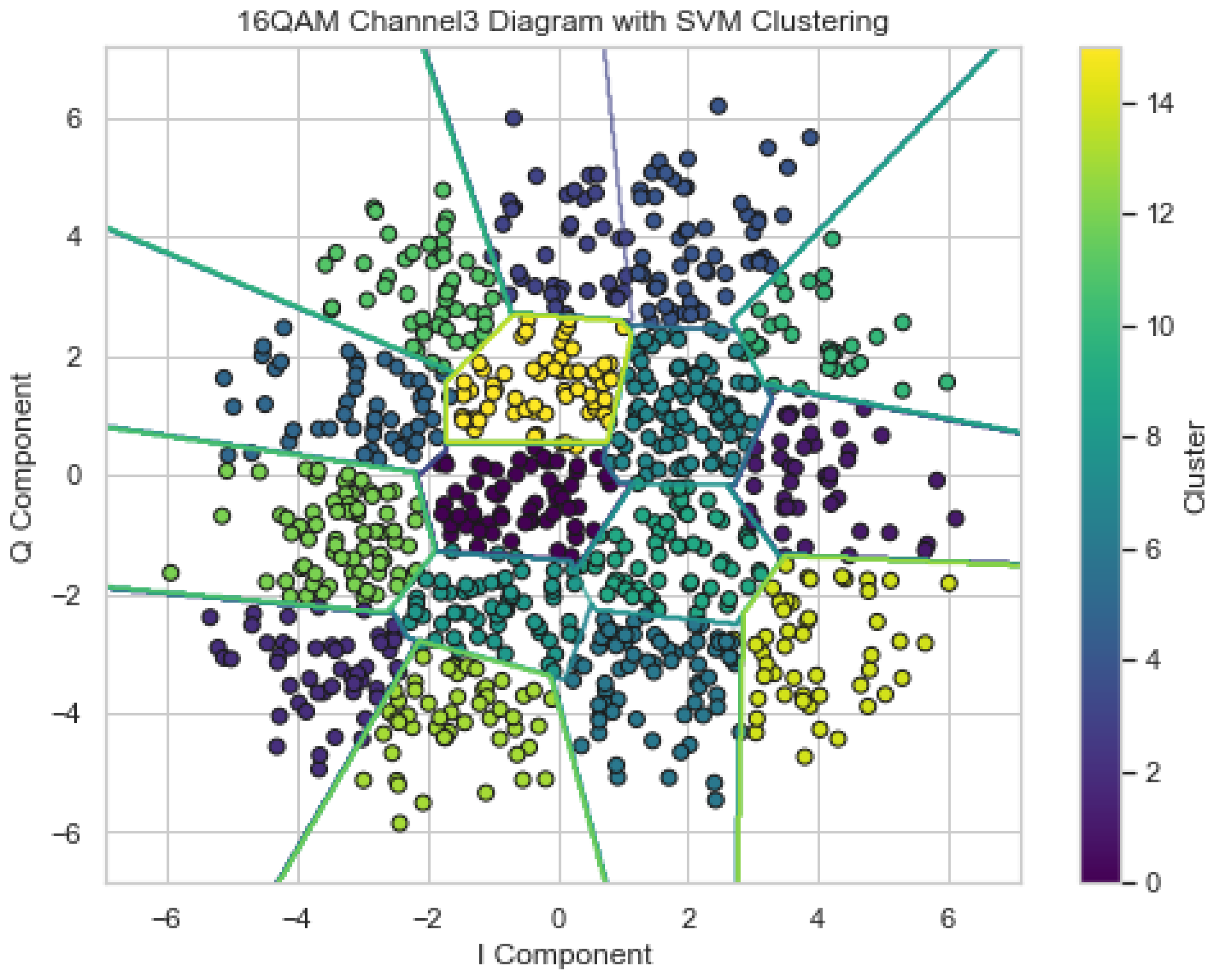
Support Vector Machines or SVM (Support Vector Machines) is a linear algorithm used for classification and regression problems. This algorithm is widely used in practice and can solve both linear and nonlinear problems. Support Vector Machines The essence of machine learning is simple: the algorithm creates a line or hyperplane that divides the data into classes. Using channel 3 as an example, a clustering diagram was constructed (Figure 8).
The SVM decision boundaries in the 16QAM Channel3 constellation diagram (Figure 8) provide a clear separation of clusters by visualizing areas corresponding to different signals. Color coding helps to understand which regions belong to which clusters. This analysis is useful for assessing the communication channel characteristics and optimizing data transmission parameters in telecommunication systems. Dark blue (cluster 1): The decision boundaries are separated by dark blue dots in the lower left corner. This area is less dense, which may indicate some distortion.
Blue (Cluster 2): The decision boundaries for the blue dots in the lower right corner indicate a region of medium signal density.
Green (Cluster 3): The decision boundaries for the green dots in the left center of the diagram separate the stable signals in this region from the other clusters.
Yellow-green (Cluster 4): The decision boundaries for the yellow-green dots in the upper part of the diagram indicate a region of medium signal density.
Yellow (Cluster 5): The decision boundaries for the yellow dots in the center of the diagram separate very dense signals from neighboring clusters.
Other Clusters. The decision boundaries for the remaining clusters follow a similar logic, separating regions of different signal density and defining areas of possible distortion or noise.
4. Conclusions
Dense Wavelength Division Multiplexing (DWDM) technology is the basis for increasing the capacity of modern optical networks. Optical performance monitoring (OPM) is necessary to ensure the reliability and quality of data transmission in DWDM systems. This article discussed the main parameters monitored in DWDM networks, their monitoring methods and implementation examples.
Key parameters such as signal power, spectral characteristics, dispersion, signal-to-noise ratio and attenuation directly affect the quality of data transmission in optical networks. The study examined the methods for measuring these parameters and their impact on the performance of DWDM networks.
Optical systems were modeled on VPI Photonics. K-means clustering and support vector machines (SVM) implemented in Python were used to analyze the data obtained using VPI Photonics. Both methods have shown high efficiency in data analysis and anomaly detection, which helps improve the monitoring and management of DWDM networks.
Thus, this study confirms the necessity and importance of optical performance monitoring techniques in DWDM networks. The implementation and development of these technologies will further improve optical communications and meet the ever-increasing demands for high-speed data transmission. Modern OPM techniques, including the use of VPI Photonics for modeling and Python for data analysis using k-means and SVM, ensure the reliability and efficiency of optical networks, which are critical to supporting global telecommunications infrastructures.
Author Contributions
Author Contributions: Conceptualization, T.A. and D.K.; methodology, T.A., D.K., A.B.; software, T.A., D.K., and M.Y.; validation, T.A.; formal analysis, T.A., A.B. and O.A.; investigation, O.A. and A.B.; resources, A.B., M.Y. and O.A.; data curation, T.A., O.A.; writing—original draft preparation, T.A., D.K., O.A.; writing—review and editing, T.A., D.K., O.A.; visualization, M.Y. and O.A.; supervision, T.A.; project administration, T.A., O.A.; funding acquisition, A.B.; M.Y.; O.A. All authors have read and agreed to the published version of the manuscript.
Funding
Not applicable.
Institutional Review Board Statement
Not applicable.
Informed Consent Statement
Not applicable.
Data Availability Statement
Not applicable.
Acknowledgments
Not applicable.
Conflicts of Interest
The authors declare that there is no conflict of interest.
References
- Wei, Z.; Wang, Zh.; Zhang, J.; Li, Q.; Zhang, J.; Fu, H.Y. Evolution of optical wireless communication for B5G/6G. Progress in Quantum Electr. 2022, 83, 100398. [Google Scholar] [CrossRef]
- Li, J. The application of optical fiber in network communication. Appl. Computat. Eng. 2024, 35, 141–146. [Google Scholar] [CrossRef]
- Yamada, Y.; Mori, T.; Matsui, T.; Kikuchi, M.; Nakajima, K. Optical Link Characteristics and Long-Term Stability of High-density Multi-Core Fiber Cables Deployed in the Terrestrial Field. In Optical Fiber Communic. Conf. (OFC) 2023, no. M3B.6, 2023. [Google Scholar] [CrossRef]
- Liu, J.; Ma, X.; Pei, G. Thermal coefficient of delay measurement of the new phase stable optical fiber. In 7th Int. Beam Instrumentation Conf. (IBIC2018); Shanghai, China, 2018; pp. 383–385. [CrossRef]
- Vergaray-Mendez, W.; Meneses-Claudio, B.; Delgado, A. Study and Analysis for the Choice of Optical Fiber in the Implementation of High-Capacity Backbones in Data Transmission. Int. J. Adv. Comput. Sci. Appl. (IJACSA) 2021, 12, 4. [Google Scholar] [CrossRef]
- Rak, J.; Girão-Silva, R.; Gomes, T.; Ellinas, G.; Kantarci, B.; Tornatore, M. Disaster resilience of optical networks: State of the art, challenges, and opportunities. Optical Switch. Net. 2021, 42, 100619. [Google Scholar] [CrossRef]
- Zhifeng, T.; Jia, Ch.; Jing, Zh.; Xu, Z. Design and Implementation of Power Communication Optical Cable Account Management System Based on GIS Technology. E3S Web Conf. 2023, 385, 02025. [Google Scholar] [CrossRef]
- Wang, D.; Jiang, H.; Liang, G.; Zhan, Q.; Mo, Y.; Sui, Q.; Li, Zh. Optical Performance Monitoring of Multiple Parameters in Future Optical Networks. J. Lightwave Tech. 2021, 39, 3792–3800. [Google Scholar] [CrossRef]
- Locatelli, F.; Christodoulopoulos, K.; Moreolo, M.S.; Fàbrega, J.M.; Nadal, L.; Spadaro, S. Spectral processing techniques for efficient monitoring in optical networks. J. Opt. Commun. Netw. 2021, 13, 158–168. [Google Scholar] [CrossRef]
- Trukhin, S.; Melnik, S.; Petrova, E. Parameters monitoring methods for the DWDM systems. In 2018 Syst. of Signals Generating and Processing in the Field of on Board Communicat.; Moscow, Russia, 2018; pp. 1–3. [CrossRef]
- Zheng, Q.; Guo, K.; Nan, J.; Deng, L.; Cheng, J. Fiber Tracking Method with Adaptive Selection of Peak Direction Based on CSD Model. Int. J. Adv. Comput. Sci. Appl. (IJACSA) 2024, 15, 6. [Google Scholar] [CrossRef]
- Lee, H.K.; Choo, J.; Kim, J. 16 Ch × 200 GHz DWDM-Passive Optical Fiber Sensor Network Based on a Power Measurement Method for Water-Level Monitoring of the Spent Fuel Pool in a Nuclear Power Plant. Sensors 2021, 21, 12. [Google Scholar] [CrossRef] [PubMed]
- Cavalcante, J.; Patel, A.; Celestino, J. Performance management of optical transport networks through time series forecasting. In IEEE 31st Int. Conf. on Adv. Informat. Net. and Appl. (AINA) 2017; pp. 152–159. [CrossRef]
- Essiambre, R.J.; Kramer, G.; Winzer, P.J.; Foschini, G.J.; Goebel, B. Capacity limits of optical fiber networks. J. Lightwave Technol. 2010, 28, 4. [Google Scholar] [CrossRef]
- de Oliveira, B.Q.; de Sousa, M.A.; Vieira, F.H.T. An optimization model based on the Firefly algorithm for optical transport network planning. Adv. Electr. Comput. Eng. 2020, 20, 2. [Google Scholar] [CrossRef]
- Dong, Z.; Khan, F.N.; Sui, Q.; Zhong, K.; Lu, C.; Lau, A.P.T. Optical performance monitoring: A review of current and future technologies. J. Lightwave Technol. 2016, 34, 525–543. [Google Scholar] [CrossRef]
- Islam, M.S.; Majumder, S.P. Optical and higher layer performance monitoring in photonic networks: Progress and challenges. In 11th Int. Conf. on Adv. Communic. Tech.; Gangwon, Korea (South), 2009; pp. 1591-1596.
- Yang, Sh.; Yang, L.; Luo, F.; Wang, Xi.; Li, B.; Du, Y. Multi-channel multi-task optical performance monitoring based on multi-input multi-output deep learning and transfer learning for SDM. Optics Communicat. 2021, 495, 127110. [Google Scholar] [CrossRef]
- Uskenbayeva, R.K.; Mukhanov, S.B. Contour analysis of external images. In ACM Int. Conf. Proceeding Series; 2020, Article 3410811. [CrossRef]
- Rottondi, C.; Barletta, L.; Giusti, A.; Tornatore, M. Machine-learning method for quality of transmission prediction of unestablished lightpaths. J. Opt. Commun. Netw. 2018, 10. [Google Scholar] [CrossRef]
- Zhuge, Q.; Zeng, X.; Lun, H.; Cai, M.; Liu, X.; Yi, L.; Hu, W. Application of machine learning in fiber nonlinearity modeling and monitoring for elastic optical networks. J. Lightwave Technol. 2019, 37, 3055–3063. [Google Scholar] [CrossRef]
- Musumeci, F.; Rottondi, C.; Nag, A.; Macaluso, I.; Zibar, D.; Ruffini, M.; Tornatore, M. An overview on application of machine learning techniques in optical networks. IEEE Commun. Surv. Tutor. 2019, 21, 1383–1408. [Google Scholar] [CrossRef]
- Liu, X.; Lun, H.; Fu, M.; Fan, Y.; Yi, L.; Hu, W.; Zhuge, Q. AI-Based Modeling and Monitoring Techniques for Future Intelligent Elastic Optical Networks. Appl. Sci. 2020, 10, 363. [Google Scholar] [CrossRef]
- Murugesan, U.; Subramanian, P.; Srivastava, Sh.; Dwivedi, A. A study of Artificial Intelligence impacts on Human Resource Digitalization in Industry 4.0. Decision Analytics J. 2023, 7. [Google Scholar] [CrossRef]
- Sun, P.; Lan, J.; Guo, Z.; Xu, Y.; Hu, Y. Improving the Scalability of Deep Reinforcement Learning-Based Routing with Control on Partial Nodes. In IEEE Int. Conf. on Acoustics, Speech and Signal Processing (ICASSP 2020); Barcelona, Spain, 2020; pp. 3557–3561. [CrossRef]
- Ayan, Z.; Alimzhan, B.; Olga, M.; Timur, Z.; Toktalyk, Z. Quality of service management in telecommunication network using machine learning technique. Indonesian J. Electr. Eng. Comput. Sci. 2023, 32, 2, 1022–1030. [Google Scholar] [CrossRef]
Figure 1.
Reference model for monitoring optical characteristics.
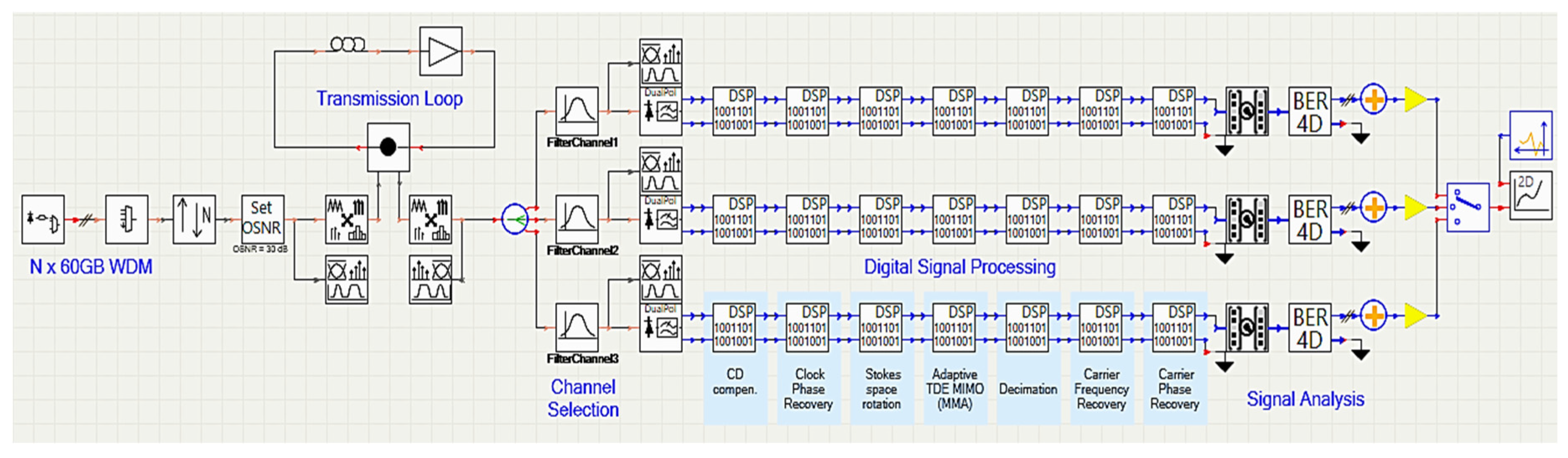
Figure 2.
Optical system analysis results for channel 1 in 400G DP-16QAM WDM c-band system.
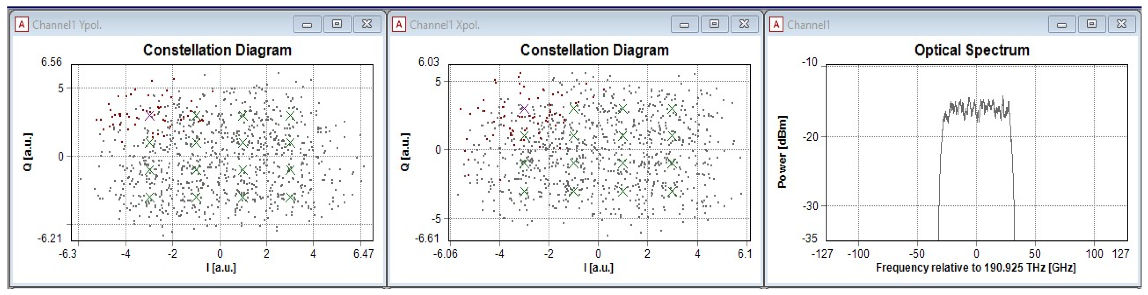
Figure 3.
Optical system analysis results for channel 2 in the C-band 400G DP-16QAM WDM system.
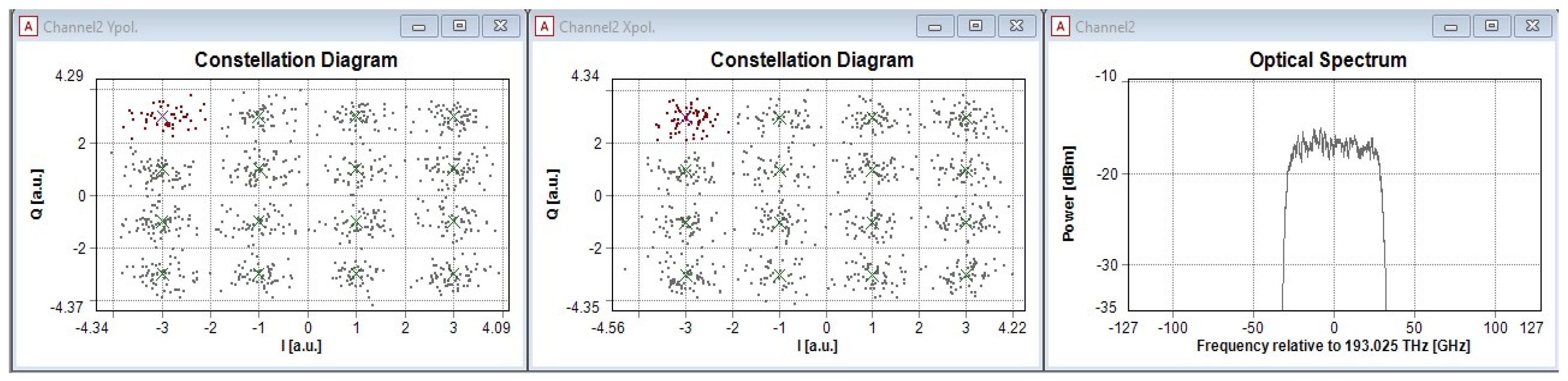
Figure 4.
Optical system analysis results for channel 3 in the C-band 400G DP-16QAM WDM system.
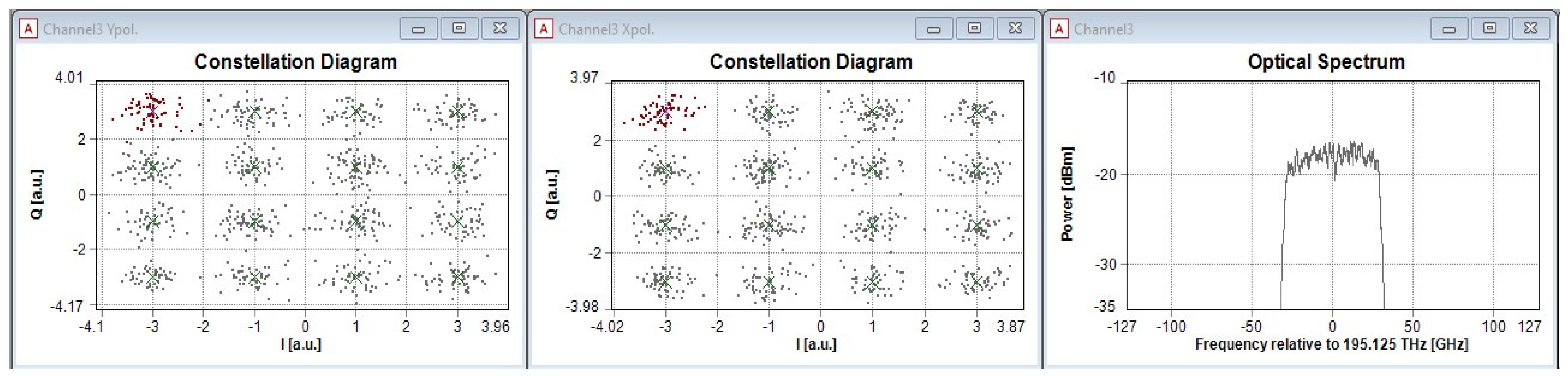
Figure 5.
Dataset fragment.
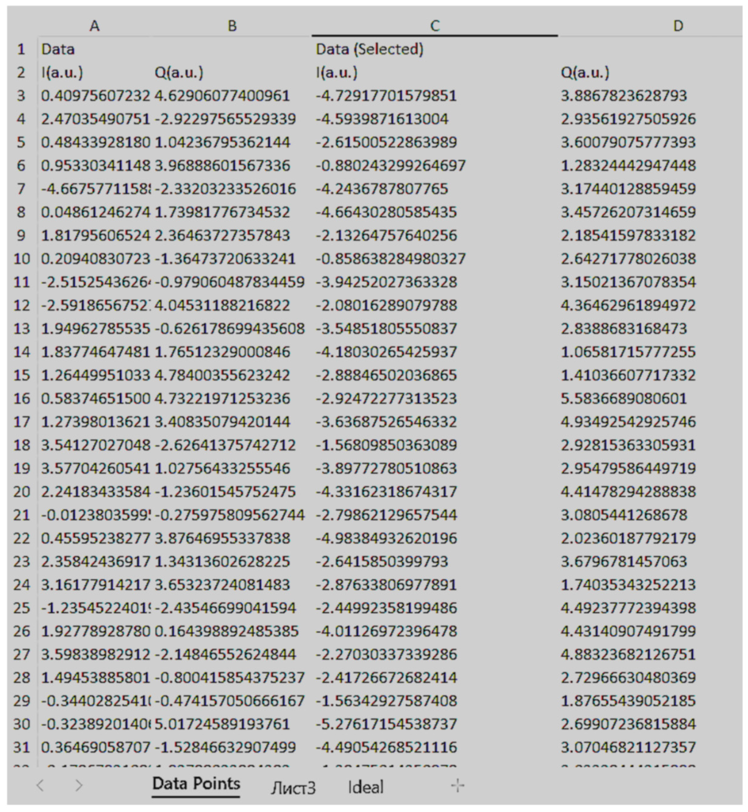
Figure 6.
16 QAM modulation according to the constellation diagram of channel 1 cluster.
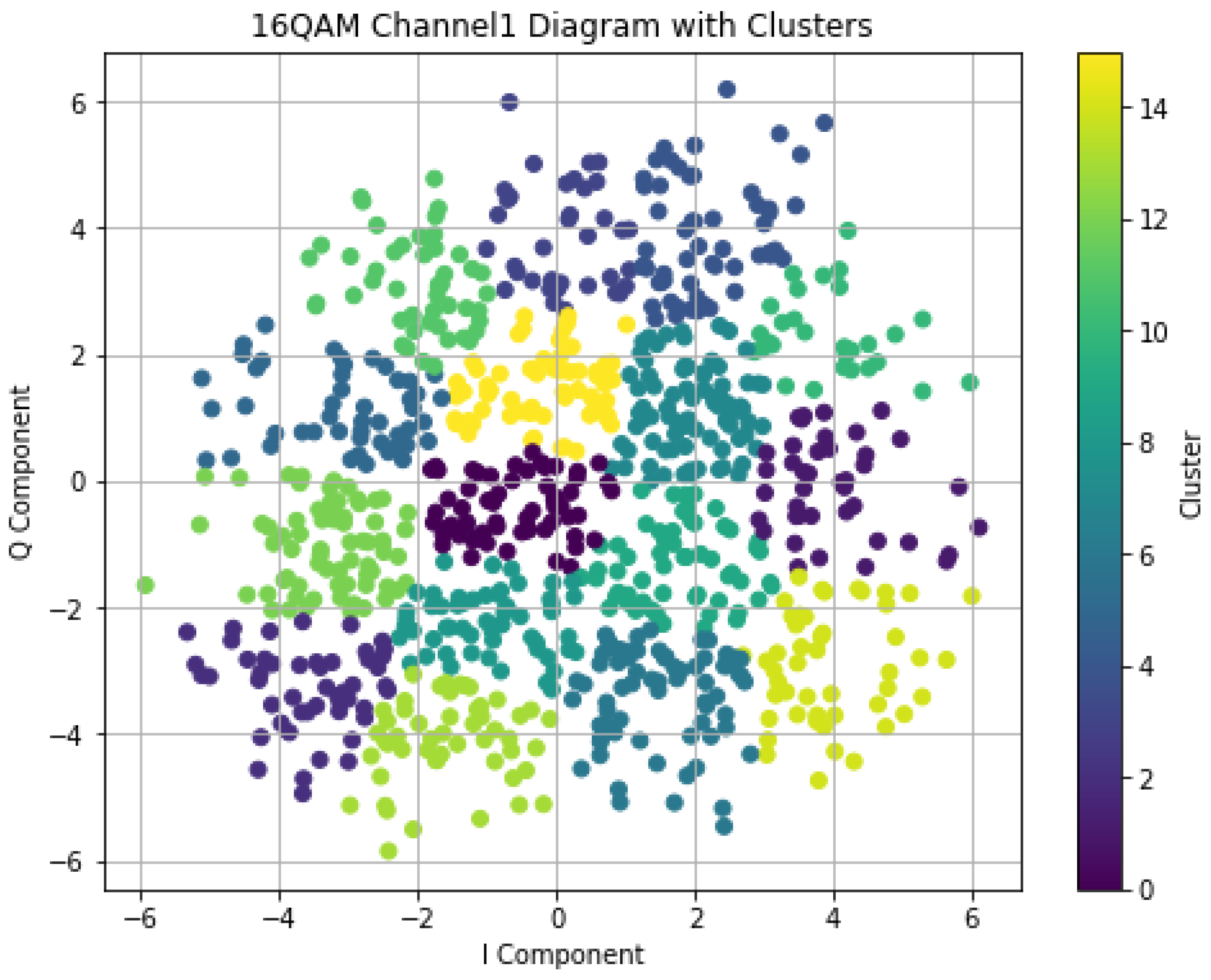
Figure 7.
16 QAM modulation according to the constellation diagram of the channel 3 cluster.
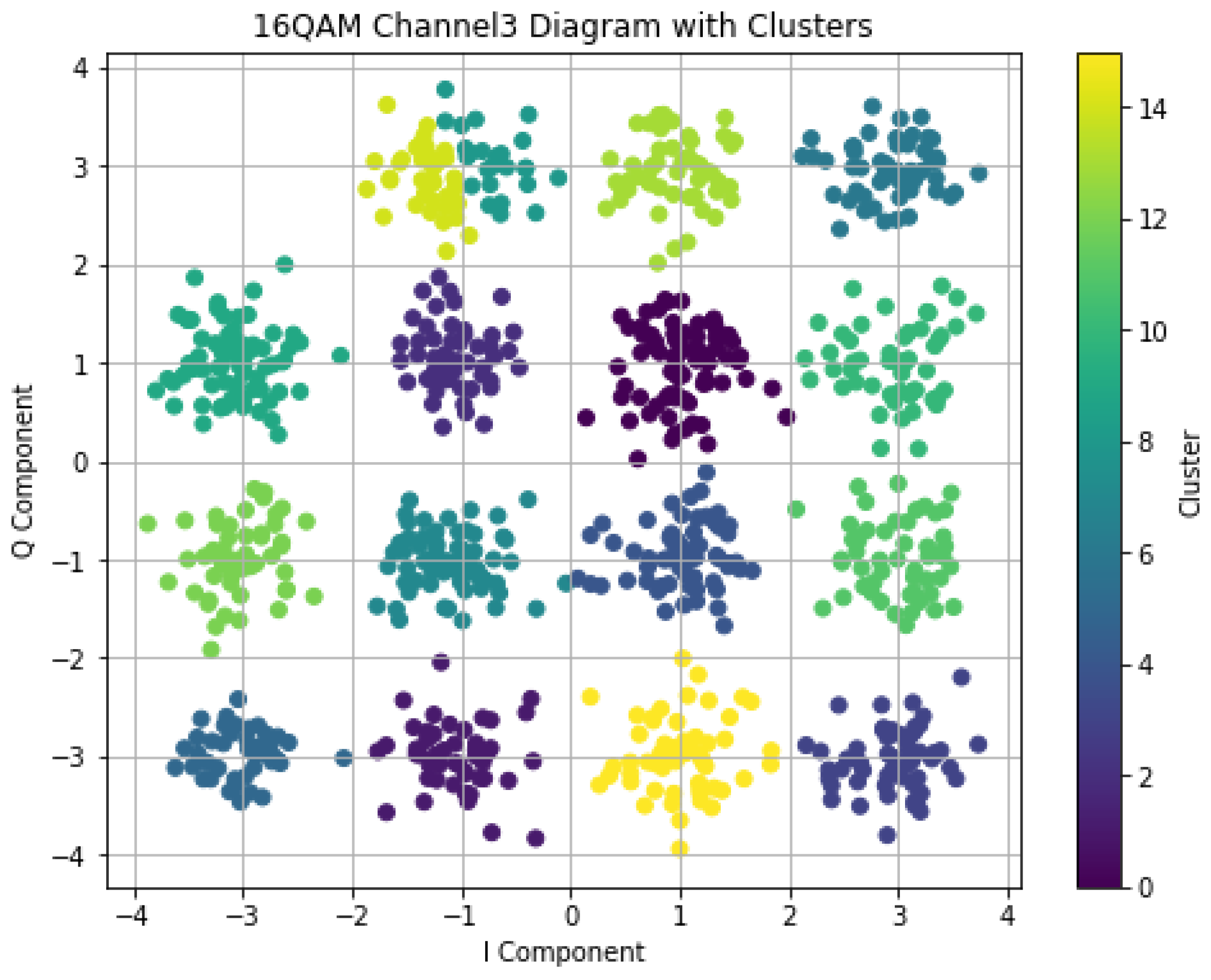
Figure 8.
16QAM 3-channel group diagram with SVM cluster.
Disclaimer/Publisher’s Note: The statements, opinions and data contained in all publications are solely those of the individual author(s) and contributor(s) and not of MDPI and/or the editor(s). MDPI and/or the editor(s) disclaim responsibility for any injury to people or property resulting from any ideas, methods, instructions or products referred to in the content. |
© 2024 by the authors. Licensee MDPI, Basel, Switzerland. This article is an open access article distributed under the terms and conditions of the Creative Commons Attribution (CC BY) license (http://creativecommons.org/licenses/by/4.0/).
Copyright: This open access article is published under a Creative Commons CC BY 4.0 license, which permit the free download, distribution, and reuse, provided that the author and preprint are cited in any reuse.


