
Submitted:
12 November 2024
Posted:
14 November 2024
You are already at the latest version
Abstract
The accuracy of satellite positioning results depends on the number of available satellites in the sky. In complex environments such as urban canyons, the effectiveness of satellite positioning is often compromised. To enhance the positioning accuracy of low-cost sensors, this paper combines the visual odometer data output by Xtion with the integrated navigation data output by the satellite receiver and MEMS IMU both in the mobile phone through adaptive Kalman filtering to improve positioning accuracy. Studies conducted in different experimental scenarios have found that in unobstructed environments, the RMSE accuracy of GNSS/IMU/visual fusion positioning improves by 50.4% compared to satellite positioning and by 24.4% compared to GNSS/IMU positioning. In obstructed environments, the RMSE accuracy of GNSS/IMU/visual fusion positioning improves by 57.8% compared to satellite positioning and by 36.8% compared to GNSS/IMU integrated positioning.
Keywords:
GNSS
; IMU
; Visual
; Adaptive filtering
; Position
1. Introduction
In modern navigation and positioning, precise and reliable positioning capabilities are a critical requirement for numerous applications, such as autonomous driving, drone flight, and mobile robot navigation. Accurate navigation and positioning primarily rely on the Global Navigation Satellite System (GNSS). This system determines the receiver’s position by measuring the distance between satellites and the receiver. By measuring the distances to at least four satellites, and using the positions of these satellites as the centers of spheres with the measured distances as radii, multiple spheres are constructed. The intersection points of these spheres represent the receiver’s position. However, in urban environments, tall buildings can obstruct satellite signals, leading to an insufficient number of available satellites. Additionally, multipath effects caused by signal reflections from building glass surfaces, as well as hardware limitations such as the cost of satellite receivers, result in reduced GNSS positioning accuracy in urban settings. To improve positioning accuracy, experts and scholars both domestically and internationally have made significant efforts. Zihan Peng et al. [1] introduced a method for enhancing smartphone GNSS positioning accuracy using inequality constraints, demonstrating that applying vertical velocity, directional, and distance constraints can significantly improve positioning accuracy. H. Zhao et al. [2] proposed a multi-view deep reinforcement learning model based on sparse representation to improve GNSS positioning accuracy in complex urban environments, and experimental results show that this algorithm significantly enhances positioning accuracy across multiple datasets. Single satellite positioning relies heavily on environmental conditions and the hardware of the satellite receiver. To enhance navigation positioning accuracy and robustness, the complementary characteristics of the satellite receiver and IMU are utilized to fuse GNSS and Inertial Navigation System (INS) [3] for integrated navigation. This not only improves the positioning accuracy of GNSS in urban environments but also enhances its robustness in complex environments. H. Qin et al. [4] proposed a graph optimization method based on virtual constraints for GNSS/IMU integrated navigation systems, and experimental results show that this method improves horizontal RMSE accuracy by approximately 30% in the absence of GNSS signals. D. Yi et al. [5] explored a smartphone GNSS/IMU integrated positioning method that combines Galileo High Accuracy Service (HAS) corrections and broadcast ephemeris, and the study shows that after incorporating IMU measurements, the precise point position (PPP) gross errors and large errors were reduced by an average of 59%. If satellite signals are lost for an extended period, civilian-grade MEMS IMUs will still diverge without satellite positioning corrections, resulting in low positioning accuracy. Consequently, multi-sensor fusion positioning has become a popular research direction among experts and scholars. Visual SLAM (Simultaneous Localization and Mapping) has become a popular research direction, and researchers have made significant contributions in this field. Beuchert J et al. [6] has proposed a factor graph design that tightly integrates raw GNSS observations (pseudo-range and carrier phase), inertial measurements, and optional LiDAR data to achieve accurate and smooth mobile robot positioning without the need for differential GNSS base stations. Yangjie Pan [7]utilized the EKF algorithm to fuse the pose information from the robot’s wheel odometry and IMU as the front-end part of the SLAM algorithm, addressing the limitation of traditional visual SLAM algorithms that overly rely on image information.
With the advancement of technology, modern smartphones are typically equipped with satellite receivers and MEMS IMU. By processing the raw observation files collected by the smartphone’s satellite receiver using pseudo-range single-point positioning(SPP) [8], single satellite positioning results can be obtained, with an error accuracy of approximately 5m in the northeast direction. When combined with the smartphone’s built-in MEMS IMU for integrated navigation positioning, the error accuracy in the northeast direction improves to approximately 3m. This paper employs adaptive filtering [9] to fuse visual odometry data from the camera with integrated navigation data collected by the smartphone, and experiments show that the positioning accuracy after visual fusion is significantly improved compared to satellite positioning and GNSS/IMU integrated navigation positioning.
2. Visual Odometry Algorithm
ORB-SLAM2 is a real-time visual SLAM system based on monocular, stereo, and RGB-D cameras, developed by Raúl Mur-Artal et al. [10] from the University of Zaragoza, Spain, for building three-dimensional maps and positioning the camera’s location and orientation without GPS signals or with limited sensor information. ORB-SLAM2 takes each frame’s image and timestamp, configuration file, and dictionary file as inputs, and outputs the camera poses corresponding to each frame, keyframes, and map points, with its framework consisting of three threads (Tracking, Local Mapping, and Loop Closing) that interact through keyframes. Upon entering the program and after the map is automatically initialized, there may be two scenarios for estimating the camera’s pose during tracking.
The first scenario involves the known translational and rotational velocities of the previous frame. The camera pose is estimated using the Perspective-n-Point (PnP) [11] method, which optimizes the camera pose based on matched 3D spatial points and 2D feature points of the current frame, formulating a least-squares problem to solve for the optimal camera pose. By calculating the Jacobian of the error concerning the pose, optimization algorithms such as the Gauss-Newton method or the Levenberg-Marquardt method can be used to iteratively solve this least-squares problem to obtain the camera pose that minimizes the projection error. For a spatial point with homogeneous coordinates , its projection coordinates in image are , its re-projection coordinates in image are , and its observed value in the image is . The re-projection error is , and the ideal re-projection process is expressed as follows:
where represents the depth of the spatial point in the camera coordinate system of image ; represents the camera intrinsic parameters; represents the pose transformation matrix of the camera from image to image . However, due to the poor initial estimation of the camera pose, the re-projection usually has some error compared to the true value. This error is defined as follows:
Typically, multiple feature points are observed under a single camera pose. Assuming we have feature points, this forms a least-squares problem for estimating the camera pose:
In order to solve this optimization problem, the first-order Taylor expansion of the objective function near the current pose is performed to obtain a linear approximation . When the error term e is a 2-dimensional coordinate error and x is the 6-dimensional camera pose error, the Jacobian matrix J will be a 2×6 matrix. According to the Lie group and algebra, the reprojection error is multiplied by the perturbation momentum at the same time, and then the derivative of the perturbation with respect to the change of e is considered, which can be obtained by using the chain rule:
is the derivative of the error with respect to the projection point.
is the derivative of the transformed point with respect to Lie algebra.
Multiply the above two equations to obtain the Jacobian matrix of the pose .After finding the Jacobian matrix, the direct method is used to solve the linear equation system so that with , and the update quantity of the optimal pose is obtained by solving .
The second scenario occurs when the translational and rotational velocities of the previous frame are unknown, or if the pose estimation from the previous frame fails, in which case nearby keyframes are used to estimate the current camera pose. After obtaining the current pose, the system enters local map tracking. It projects the local map points generated from the previous frame onto the current frame for tracking to further optimize the pose and creates keyframes based on predefined conditions. The local mapping thread receives keyframes from the tracking thread and generates new map points using the co-visibility relationships of the keyframes. It searches for and merges map points from adjacent keyframes, then perform local map optimization, removes redundant keyframes, and establishes more connections between existing keyframes. This process generates more reliable map points, optimizes the poses of co-visible keyframes and their map points, stabilizes tracking, and ensures more accurate poses for keyframes involved in loop closure. The loop closing thread is used to determine whether the camera has returned to a previously visited location, thereby adjusting the map and pose to prevent map drift caused by accumulated errors. The Bag of Words (Bow) model is used to search the keyframe database for loop closure candidate keyframes corresponding to the current keyframe. Continuity checks are performed on the selected loop closure candidate keyframes to ensure the reliability of the loop closure. If a loop closure is detected, the Sim3 transformation between the current frame and the loop closure candidate frame is used to correct the current keyframe. Moreover, global optimization is performed on the poses of all keyframes and map points to improve the accuracy of the map and pose estimation.
3. Overall Design of GNSS/IMU/Visual Fusion Positioning
By processing inertial navigation system mechanization to the specific force and angular velocity outputs from the IMU, the changes in the position, velocity, and attitude of the carrier can be obtained. This method provides accurate positioning in the short term and is not affected by external interference. Since the navigation information is generated through integration, the positioning error gradually increases over time. To reduce the positioning error and enable long-term positioning, adaptive filtering is used to fuse the outputs of the IMU and GNSS. GNSS can provide relatively accurate positioning information over the long term, but it is susceptible to factors such as high-rise building obstructions. Based on the physical characteristics of the IMU and satellite receiver, an adaptive filtering fusion approach can be designed. The difference between the GNSS measurement information and the predicted position and velocity from the INS is used as the innovation for measurement updates. This allows for the estimation and feedback correction of relevant parameters in the state equation, thereby achieving closed-loop compensation for the IMU parameters. The state equation can be formulated as follows:
where: represents the INS position error; represents the INS velocity error; represents the INS attitude error; represents the gyroscope bias; represents the accelerometer bias; represents the gyroscope scale factor error; represents the accelerometer scale factor error. The observation equation for the loosely coupled integration can be derived from the GNSS positioning results as follows:
where: represents the INS position output; represents the GNSS position observation output; the measurement noise vector is zero-mean white noise, satisfying and . However, in practical applications, there are errors in obtaining the structural parameters and noise statistical parameters of the stochastic system. These errors can reduce the filtering accuracy and even cause filter divergence. Therefore, it is necessary to effectively estimate the measurement noise covariance matrix . By reconstructing the measurement noise covariance matrix through weighted recursive estimation, it can be derived as follows:
where is referred to as the fading factor, with smaller values indicating stronger adaptability, commonly set to [12]. GNSS and IMU data are combined using adaptive filtering to obtain a simplified loosely coupled navigation pose, which is then further fused with the pose data from visual odometry using adaptive filtering. Due to the difference in sampling frequencies, the pose data output from the integrated navigation system is at 1Hz, while the pose data from visual odometry depends on keyframes and may not be at 1Hz. To address the issue of pose timestamp misalignment caused by different sampling frequencies, the timestamps of the integrated navigation and visual outputs are first converted to GPS week numbers and seconds of the week, and then processed using interpolation to achieve time synchronization. The final fusion of the integrated navigation pose and visual odometry pose can be represented by the state equation as shown in Equation (4), where:
where represents the visual position error; represents the visual velocity error. The observation equation is:
where represents the visual position observation; represents the integrated navigation position (). The overall framework of GNSS, IMU, and visual fusion can be illustrated as shown in Figure 1.
4. Experimental Analysis and Results
4.1. Experimental Analysis
The data collection for the IMU and GNSS receiver was conducted using a Huawei NOVA 8 Pro smartphone. The built-in MEMS IMU is the Bosch BMI 260. The GNSS receiver sensor is the Hi 1105, integrates multiple functional modules, including Wi-Fi, Bluetooth, and GNSS, and supports various satellite navigation systems such as GPS L1 CA/L5, GLONASS L1OF, BeiDou B1I/B1C/B2A, Galileo E1/E5a, SBAS, QZSS L1/L5, and IRNSS SPS-L5, enabling positioning. During the experiment, data collection using the smartphone involved the use of the apps rinex ON and PSINS. The purpose of rinex ON was to collect satellite observation files. PSINS, developed by Gongmin Yan’s team at Northwestern Polytechnical University, is used to collect integrated navigation files. Before officially starting the integrated navigation data collection, PSINS requests location permissions from the system. It calculates the smartphone’s attitude using data output from the phone’s IMU. Due to the lack of an initial alignment function, the attitude results serve as the initial attitude for subsequent integrated navigation. The camera used is an Xtion, which needs to be calibrated before conducting experiments. First, the camera captures images of a black-and-white chessboard at different distances and angles. After saving the images in a folder, the Stereo Camera Calibrator tool in MATLAB 2022a is used for calibration. The calibrated camera intrinsic parameters are then updated in the ASUS.yaml file of ORB-SLAM2. With calibration complete, experiments are conducted. Since the pose output by the camera odometer is relative and does not coincide with the absolute position generated by the integrated navigation, satellite positioning data must be used to correct the pose generated by the camera odometer before performing AKF fusion with the integrated navigation. Figure 2 shows the deviation between the satellite positioning results and the visual odometer positions.
Data collected by the BD930 satellite receiver, a product of Beijing Fuxing Yuanhang Company, is used as ground truth. BD930 includes a base station and a rover station. The base station is fixed at a high location, while the rover station performs mobile measurements. Differential positioning of data collected by the base and rover stations can achieve centimeter-level accuracy. The experimental equipment setup is shown in Figure 3.
In Figure 3, the left image shows the installation of the base station receiver, while the right image shows the rover station receiver (white), with the smartphone beside it and the camera below. The sensor parameters obtained from the product company’s official website and our measurements are shown in Table 1.
4.2. Experimental Results
To avoid experimental randomness, six sets of experiments were conducted. The experimental sites were chosen as a basketball court and a football field, with the experiments conducted during the afternoon to evening period. Based on the experimental environment, the six sets of experiments were divided into two groups: obstructed and unobstructed, with three sets in each group. The unobstructed group received more usable satellites, and the ample lighting facilitated the selection of keyframes by the camera. In contrast, the obstructed group had fewer usable satellites, and the dim lighting hindered the selection of keyframes by the camera. Different experimental environments were set up to observe and analyze the feasibility and robustness of GNSS, IMU, and visual sensor fusion under varying conditions. The satellite positioning results, GNSS/IMU integrated positioning results, and GNSS/IMU/visual fusion positioning results were analyzed and compared. The position trajectory solution for one set of data is shown in Figure 4.
Based on Table 1, the single-point positioning data collected by the mobile satellite receiver exhibits an excessive upward positioning error, exceeding 15m. Therefore, subsequent analyses do not consider the vertical error. After analyzing and processing these six sets of collected data, the results include satellite positioning, GNSS/IMU integrated positioning, and GNSS/IMU/visual fusion positioning. The results obtained from these three positioning methods are compared with the ground truth to obtain the Standard Deviation (STD) and Root Mean Square Error (RMSE), as shown in Table 2 and Table 3.
where represents the overall STD; represents the eastward STD; represents the northward STD. Similarly, the RMSE can be obtained.
From Table 2 and Table 3, it can be observed that both satellite positioning and GNSS/IMU integrated positioning achieve satisfactory results in unobstructed environments. The fusion positioning, which incorporates visual odometry data, performs even better. The RMSE of the fusion positioning shows an improvement in accuracy of the most up to 61.3% compared to satellite positioning and GNSS/IMU integrated positioning. In obstructed environments, the accuracy of satellite positioning and GNSS/IMU integrated positioning deteriorates. Despite the influence of lighting conditions, the accuracy significantly improves after incorporating visual data. The RMSE of the fusion positioning shows an improvement in accuracy of the most up to 59.7% compared to satellite positioning and GNSS/IMU integrated positioning.
5. Conclusions
This study analyzes the positioning accuracy of different sensor fusion methods in various environments, using a smartphone’s satellite receiver, MEMS IMU, and an Xtion for experiments. By using different methods to fuse the raw data collected from the smartphone and camera through adaptive filtering, three positioning results can be obtained: satellite positioning, GNSS/IMU integrated positioning, and GNSS/IMU/visual fusion positioning. An analysis and comparison of these three positioning methods reveal that in unobstructed environments, the STD accuracy of the GNSS/IMU/Visual fusion positioning improves by 44.9% compared to satellite positioning and by 21.2% compared to GNSS/IMU integrated positioning. The RMSE accuracy of the GNSS/IMU/Visual fusion positioning improves by 50.4% compared to satellite positioning and by 24.4% compared to GNSS/IMU integrated positioning. In obstructed environments, the STD accuracy of the GNSS/IMU/Visual fusion positioning improves by 54.9% compared to satellite positioning and by 35.5% compared to GNSS/IMU integrated positioning. The RMSE accuracy of the GNSS/IMU/Visual fusion positioning improves by 57.8% compared to satellite positioning and by 36.8% compared to GNSS/IMU integrated positioning.
Author Contributions
Ao Liu is responsible for conducting the entire experiment and writing the entire paper. Hang Guo, Jian Xiong, and Min Yu are responsible for constructing the overall thought framework of the paper. Huiyang Liu provides guidance on the use of ORB-SLAM2. Pengfei Xie assists in collecting experimental data.
Funding
This research was funded by the National Natural Science Foundation of China (Grant Nos. 62263023;41764002; 62161002).
Institutional Review Board Statement
Not applicable.
Informed Consent Statement
Not applicable.
Data Availability Statement
Not applicable.
Acknowledgments
Thanks to the National Natural Science Foundations of China (62263023, 41764002 and 62161002) and the Graduate Innovation Special Fund of Jiangxi province of China (YC2024-S143) for their support for this paper. Corresponding author: Professor Hang Guo, e-mail: hguo@ncu.edu.cn.
Conflicts of Interest
The authors declare no conflict of interest.
References
- Z. Peng, Y. Gao, C. Gao, R. Shang, and L. Gan, “Improving smartphone GNSS positioning accuracy using inequality constraints,” Remote Sens., vol. 15, no. 8, pp. 2062-2084, 2023. [CrossRef]
- H. Zhao et al., “Improving performances of GNSS positioning correction using multiview deep reinforcement learning with sparse representa tion,” GPS Solut., vol. 28, no. 3, pp. 98–120, 2024.
- Mohamed A H, Schwarz K P. Adaptive Kalman filtering for INS/GPS[J]. Journal of geodesy, 1999, 73: 193-203.
- Qiu, H.; Zhao, Y.; Wang, H.; Wang, L. A Study on Graph Optimization Method for GNSS/IMU Integrated Navigation System Based on Virtual Constraints. Sensors, vol. 24, no. 13, pp. 4419-4436,2024. [CrossRef]
- Yi D et al., “Precise positioning utilizing smartphone GNSS/IMU integration with the combination of Galileo high accuracy service (HAS) corrections and broadcast ephemerides”. GPS Solut., vol. 28, no. 3, pp. 140–155, 2024.
- Beuchert J, Camurri M, Fallon M. Factor graph fusion of raw GNSS sensing with IMU and lidar for precise robot localization without a base station[C]//2023 IEEE International Conference on Robotics and Automation (ICRA). IEEE, 2023: 8415-8421.
- Yangjie P. Vision and Multi-sensor Fusion BasedMobile Robot Localization in Indoor Environment [D].Zhejiang University,2019.
- FANG Xinqi, FAN Lei. Accuracy analysis of BDS-2/BDS-3 standard point positioning[J]. GNSS World of China, 2020, 45(1): 19-25.
- Xueyuan L,Lili L,Yunyun D,et al. Improved Adaptive Filtering Algorithm for GNSS/SINS Integrated Navigation System[J]. Geomatics and Information Science of Wuhan University,2023,48(01):127-134.
- R. Mur-Artal and J. D. Tardós, "ORB-SLAM2: An Open-Source SLAM System for Monocular, Stereo, and RGB-D Cameras," in IEEE Transactions on Robotics, vol. 33, no. 5, pp. 1255-1262, Oct. 2017. [CrossRef]
- Q. Sun et al., "Efficient Solution to PnP Problem Based on Vision Geometry," in IEEE Robotics and Automation Letters, vol. 9, no. 4, pp. 3100-3107, April 2024. [CrossRef]
- Yan G, Liu P, Li Z, et al. An adaptive Kalman filter based on soft Chi-square test[J]. Navig. Positioning Timing, 2023, 10: 81-86.
Figure 1.
GNSS/IMU/Visual Fusion Positioning Algorithm Flowchart.
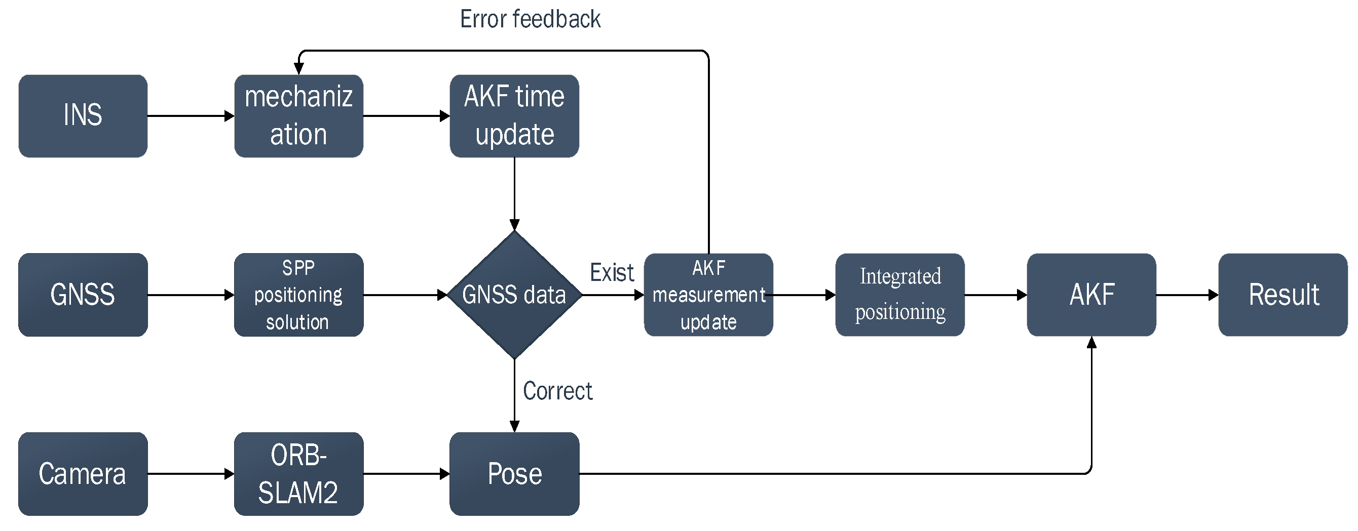
Figure 2.
Deviation between Satellite Positioning and Visual Odometer Poses.
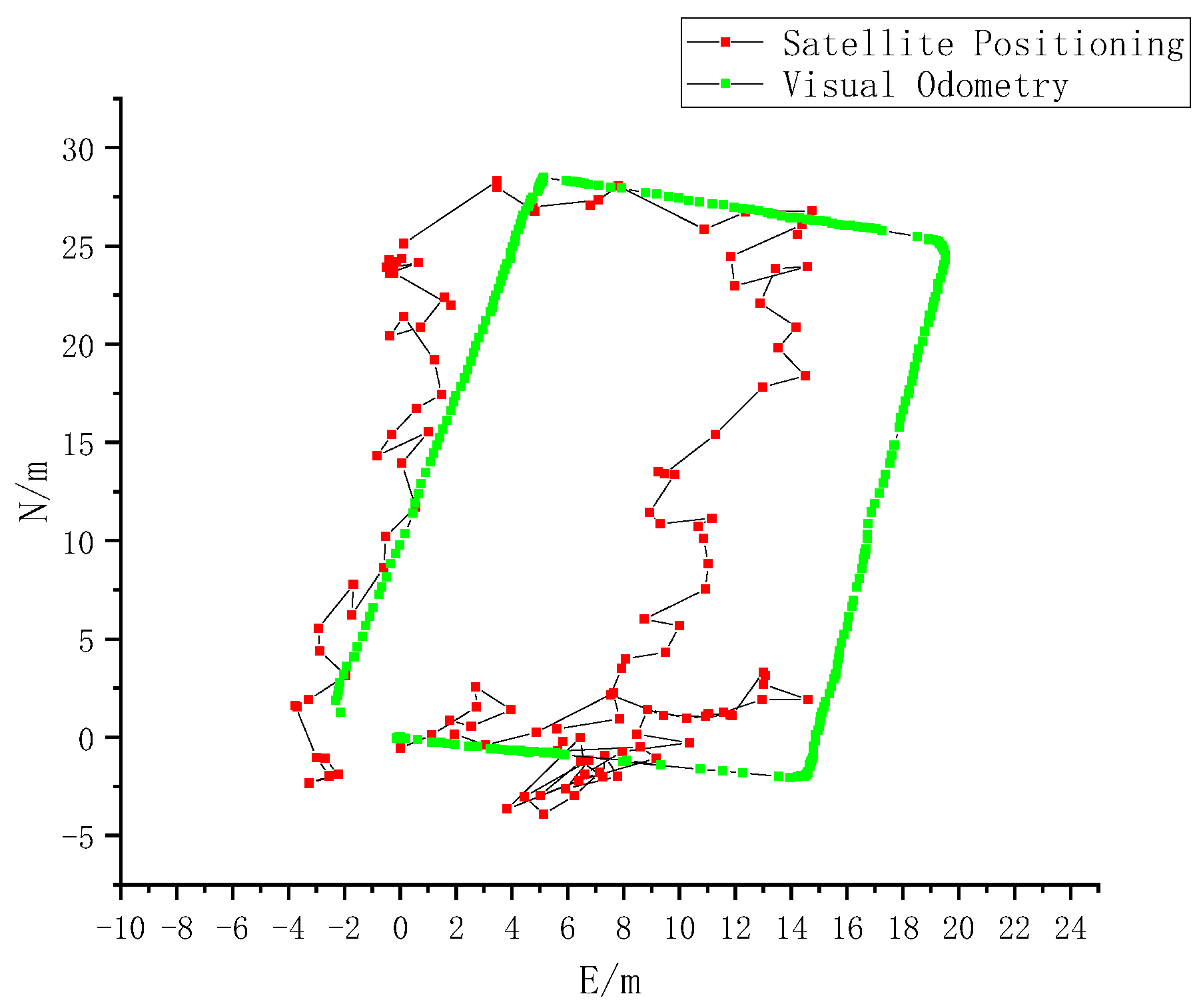
Figure 3.
Experimental Equipment Setup.
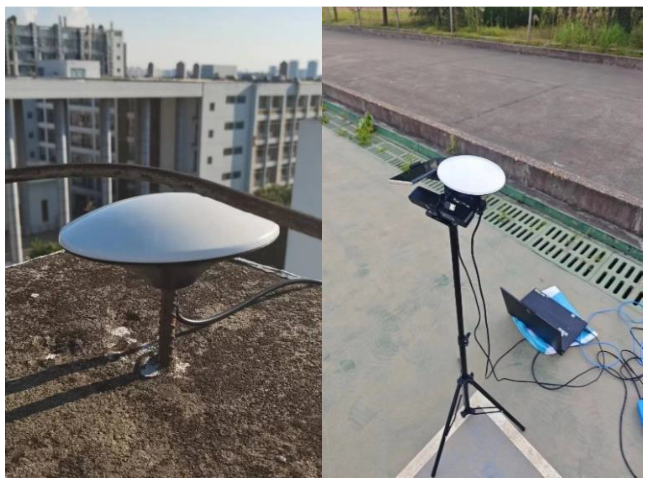
Figure 4.
Position Trajectory Solution Diagram.
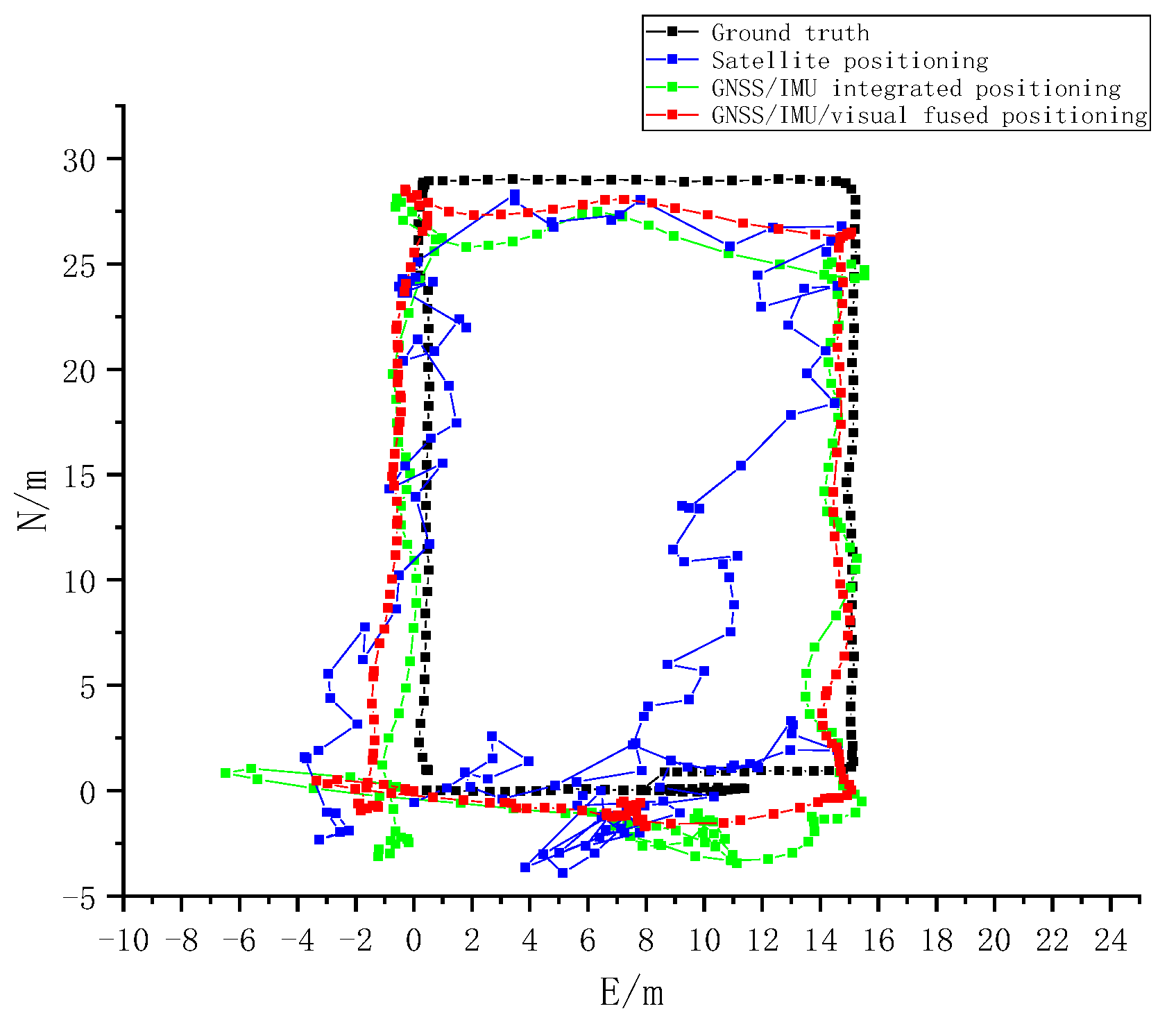

Table 1.
Sensor Parameters.
| Sensor | Parameter | Technical data |
|---|---|---|
| Bosch BMI 260 | Programmable measurement range | |
| Zero bias | ||
| Sensitivity Error | ||
| Noise density | ||
| Hi 1105 | Eastward Positioning Accuracy(SPP) | |
| Northward Positioning Accuracy(SPP) | ||
| Upward Positioning Accuracy(SPP) | ||
| Xtion | Eastward Positioning Accuracy(After Correction) | |
| Northward Positioning Accuracy(After Correction) | ||
| BD930 | Eastward Positioning Accuracy(Differential Positioning) | |
| Northward Positioning Accuracy(Differential Positioning) |
Table 2.
Navigation Positioning Solution STD and Its Accuracy Improvement.
| Environment | Experimental sequence | Satellite positioning /m | GNSS/IMU integrated positioning /m | GNSS/IMU/visual fused positioning /m |
Accuracy improvement (satellite positioning)/% | Accuracy improvement (integrated positioning)/% |
|---|---|---|---|---|---|---|
| Unobstructed | First | 2.8945 | 2.3597 | 1.7611 | 39.2 | 25.4 |
| Second | 3.3586 | 1.9683 | 1.4131 | 57.9 | 28.2 | |
| Third | 5.2161 | 3.6935 | 3.147 | 39.7 | 14.8 | |
| Average | 3.8231 | 2.6738 | 2.1071 | 44.9 | 21.2 | |
| Obstructed | Fourth | 6.1739 | 5.4834 | 3.0609 | 50.4 | 44.2 |
| Fifth | 9.5697 | 4.7627 | 4.2512 | 55.6 | 10.7 | |
| Sixth | 6.9074 | 5.5784 | 2.8931 | 58.1 | 48.1 | |
| Average | 7.5503 | 5.2748 | 3.4017 | 54.9 | 35.5 |
Table 3.
Navigation Positioning Solution RMSE and Its Accuracy Improvement.
| Environment | Experimental sequence | Satellite positioning /m | GNSS/IMU integrated positioning /m | GNSS/IMU/visual fused positioning /m |
Accuracy improvement (satellite positioning)/% | Accuracy improvement (integrated positioning)/% |
|---|---|---|---|---|---|---|
| Unobstructed | First | 4.1966 | 3.9723 | 2.7378 | 34.3 | 31.1 |
| Second | 4.7599 | 2.4307 | 1.8422 | 61.3 | 24.2 | |
| Third | 8.482 | 5.0603 | 4.0758 | 51.9 | 19.5 | |
| Average | 5.8128 | 3.8178 | 2.8853 | 50.4 | 24.4 | |
| Obstructed | Fourth | 9.0871 | 6.7426 | 3.6645 | 59.7 | 45.7 |
| Fifth | 11.6945 | 5.7192 | 4.7475 | 59.4 | 17 | |
| Sixth | 11.2584 | 8.9399 | 5.1084 | 54.6 | 42.9 | |
| Average | 10.68 | 7.1339 | 4.5068 | 57.8 | 36.8 |
Disclaimer/Publisher’s Note: The statements, opinions and data contained in all publications are solely those of the individual author(s) and contributor(s) and not of MDPI and/or the editor(s). MDPI and/or the editor(s) disclaim responsibility for any injury to people or property resulting from any ideas, methods, instructions or products referred to in the content. |
© 2024 by the authors. Licensee MDPI, Basel, Switzerland. This article is an open access article distributed under the terms and conditions of the Creative Commons Attribution (CC BY) license (http://creativecommons.org/licenses/by/4.0/).
Copyright: This open access article is published under a Creative Commons CC BY 4.0 license, which permit the free download, distribution, and reuse, provided that the author and preprint are cited in any reuse.


