
Submitted:
08 November 2024
Posted:
11 November 2024
You are already at the latest version
Abstract
In the present work, we consider a seven-parameter, three-dimensional, autonomous, cubic polynomial system of nonlinear ordinary differential equations, generalizing the recently studied quadratic polynomial Hopf–Langford type systems. First, by introducing polar coordinates in its phase space, we show that the regarded system can be reduced to a two-dimensional Liénard system, which corresponds to a second-order Liénard equation. Then, we present (in explicit form) polynomial first and second integrals of Liénard systems of the considered type identifying those values of their parameters for which these integrals exist. It is also proved that a generic Liénard equation is factorizable if and only if the corresponding Liénard system admits a second integral of a special form. It is established that each Liénard system corresponding to a Hopf–Langford system of the considered type admits such a second integral and hence the respective Liénard equation is factorizable.
Keywords:
Dynamical systems
; Liénard system and equation
; first integrals
; second integrals
; Darboux polynomials
; exact solutions
1. Introduction
The qualitative study of turbulence (spatial complex and temporally “random” fluid motion) using dynamical systems theory was first applied by Hopf [1]. In more detail, he reduced the dynamics of the Navier–Stokes equations for turbulent flow to those on an attractor, and after that studied their dynamics (bifurcations) in the context of nonlinear finite-dimensional flows and maps. Later on, in 1971, Ruelle and Takens [2] suggested that the mechanism of a finite sequence of bifurcations is that underlies turbulence. It is intuitively obvious that, although a low-dimensional model simplifies and significantly restricts the full behaviour of a flow with more modes, the low-dimensional model can provide only qualitative information on key mechanisms and the key features of a complex turbulent flow. Thus, the following questions naturally arise: 1) How well does this low-dimensional model approximate the attractor of the original system? and 2) Can we obtain systems that are as small as possible, but will still yield relevant results? The relative simplicity of this kind of model explains why its use continues to this day. To proceed with these crucially important questions, an interaction between physics, mathematics, and computer science as well as a comprehensive approach to the problem is essential. The earliest turbulence model proposed by Hopf in [1] was modified by Langford first in private communication (see [3] p. 106]) and then in a journal article [4]. This modified model predicts regular oscillations due to a Poincaré–Andronov–Hopf bifurcation [3] and chaotic behaviour for a specific choice of the parameters [5,6,7]. However, addressing this issue requires a further extension of the model to the so-called generalized Hopf–Langford (GHL) systems. Such extended models have been proposed recently in [8,9,10,11] and are being analytically and numerically studied, see [8,9,10,11,12,13,14]. The results obtained within the GHL systems provide cues for the transition from simple to complex oscillatory phenomena. Thus, from a more global perspective, the GHL systems underline the links between similar dynamic phenomena occurring in different settings — physical, chemical and biological.
In the present paper, slightly extending the Hopf–Langford type systems studied in [9,10,11], we consider the cubic polynomial differential system
where, as usual, the overdots denote differentiation with respect to the independent variable t, and , , , , , and are real numbers.
The motivation for the current work is to find first and second integrals of the system (1) as their existence and specific forms would provide a better understanding of the dynamics (local and global bifurcation behaviour) and stability of such a nonlinear dynamical system. Moreover, the Darbouxian theory of integrability provides a link between the integrability of polynomial vector fields and the number of invariant algebraic curves that they have.
The paper is organized as follows. In Section 2, by introducing polar coordinates in the phase space of the system (1), we show that it reduces to a two-dimensional Liénard system, which corresponds to a second-order Liénard equation. Then, in Section 3, we present first and second integrals of this Liénard system identifying the values of the involved parameters for which these integrals exist. In Section 4, we show that a generic Liénard equation is factorizable if and only if the corresponding Liénard system admits a second integral of a special form. In Section 5, using the established first and second integrals, we give some typical examples of phase portraits and particular solution curves of Liénard systems of the form (12). In Section 6, we briefly discuss the obtained results.
2. Dimensional Reduction of the Extended Hopf–Langford System (1)
It is easy to verify that upon the transformation of the variables of the form
i.e., upon introducing polar coordinates in the phase space , the system (1) takes the form
where . Thus, the regarded system splits into the equation that gives
where is an arbitrary real constant, and the two-dimensional amplitude system
whose associated vector field reads
The general solution of the system (6) & (7) is readily obtained to be
where , and are arbitrary real constants.
So, hereafter we assume .
Next, substituting expressions (8) for the variable y and its derivative in the second one of equations (4), one arrives at the polynomial Liénard equation (see [15])
with
and
in the considered case. Equation (9) is equivalent to the following, defined in the phase plane , , differential system
which is frequently called the Liénard system, with
as the associated vector field. Notice that in the passage from the equation (9) to the system (12), we kept, for the sake of simplicity, the same notation, ”y”, for the newly introduced dependent variable as those used in the system (4). Actually, under the transformation
the system (4) maps into the system (12) in which the functions and are given by the equations (10) and (11), respectively. Clearly, the inverse transformation is
3. First and Second Integrals of the Liénard System (12)
To specify the terminology, let us first recall the definitions of the first and second integrals of a real planar polynomial differential system
where is the ring of polynomials in x and y with real coefficients.
Definition 1.
A function is said to be first integral of the system (16) if
Let be a first integral of a differential system of the form (16). From the condition (17) it is evident that on the solutions of this system. In other words, each solution of the regarded system lies on a level set , determined by certain real constant c, of its first integral. In this sense, the phase portrait of such a system may be considered completely determined.
Definition 2.
A function is said to be second integral of the system (16) if there exist a polynomial , called the cofactor, such that
In the context of dynamical systems theory, the second integrals are known in the literature under several different names, see the comments on p. 46 in [16]. Here, they will also be referred to as the Darboux polynomials or invariant algebraic curves of system (16).
According to Poincaré, the basic problem of nonlinear dynamics is studying near-integrable differential systems. In general, the dynamics of higher-dimensional systems is difficult to study. But, if a system has functionally independent first (and second) integrals, then its dynamics can be reduced to that of a lower-dimensional system, which is easier to investigate. That is why the problem of the existence and determination in an explicit form of first and second integrals of a given dynamical system is important and attracts the interest of many researchers, see, e.g., [10,11,16,17,18,19] and the references therein.
Consider now a generic Liénard equation
together with the corresponding Liénard system consisting of the two coupled equations
and its associated vector field
As usual, this vector field will also be regarded as an operator acting on the smooth functions defined on some open subset of the phase plain .
It is well-known (cf., e.g., [20]) that each Liénard system (20) is Hamiltonian, with a first integral
under the condition . Indeed, if , then it is easy to check that
In the case of the system (12), we end up with the following result.
Proposition 1.
Each system of the form (12) in which the parameters involved in the functions and defined by the equations (10) and (11), respectively, obey the conditions
admits a first integral of the form
Proof.
Another first integral arises when the parameters and involved in a system of the form (12) are not equal and .
Before presenting this result as well as the results concerning the derivation of second integrals, however, let us make a remark. Given a nonlinear differential system, no universal method exists for constructing its first and second integrals. In the present work, we take some ”promising” polynomials with arbitrary coefficients and try to satisfy the conditions (17) or (18) that in the case of a system of the form (12) leads to an over-determined system of algebraic equations whose solutions (if exist) identify those values of the parameters of the regarded system for which first or second integrals exist.
All the results presented below in the Propositions , and are obtained following this approach.
Proposition 2.
Each system of the form (12) in which the parameters involved in the functions and defined by the equations (10) and (11), respectively, obey the conditions
admits a first integral of the form
where
Proof.
Actually, and are second integrals (Darboux polynomials) of any system of the form (12) for which the conditions (26) are satisfied. Indeed, if this is the case, then it is easy to check that
Hence, according to Definition 2, and are second integrals of the respective systems of form (12). Notably, the second one of the above relations is valid even if the conditions (26) are not satisfied meaning that any Liénard system that corresponds to a generalized Hopf–Langford system of the form (1) has a second integral.
Proposition 3.
Each Liénard system of the form (12) admits the function
as a second integral of cofactor
Proof.
Below, a family of Liénard systems of the form (12) with is specified which admits second integrals in addition to that formulated in Proposition 3.
Proposition 4.
Any Liénard system of the form (12) for which
admits the function
as a second integral (Darboux polynomial) of cofactor
Proof.
Hence, according to Definition 2, is a second integral of the respective system of the form (12) of cofactor . □
4. Factorization of the Liénard Equation
Definition 3.
An equation of the form (19) is said to be factorizable if there exist tow functions and of the dependent variable x such that
Proposition 5.
Proof.
The proof of this assertion is straightforward. It suffices to perform the differentiations in the right-hand side of the Equation (38) and compare the obtained result with the left-hand side of this relation. □
Proposition 6.
Let a Liénard type equation of the form (19) be factorizable, i.e., there exist two functions and such that it can be represented in the form (38). Then, the functions
satisfy the relation
that is, J is a second integral (Darboux polynomial) of the corresponding Liénard system (20) with cofactor Λ.
Proof.
Proposition 7.
Let the functions , and be such that the Liénard system (20) admits a second integral (Darboux polynomial) of the form
with a given cofactor . Then, the corresponding Liénard equation (19) is factorizable.
Proof.
Let a function given by the expression (42) be a Darboux polynomial with cofactor of a Liénard system (20) determined by the functions and , that is
It is easy to see now, that any tow functions of the form (45) can be represented in the form (39) taking
Therefore, according to Proposition 5, the corresponding Liénard equation is factorizable since the identity
holds for any two functions and . □
Combining the above propositions, we can formulate the following theorem.
Theorem 1.
It should be noted that the factorizability of Liénard type equations has been studied in a number of works (see, e.g., [21] and the relevant references therein). However, to the best of our knowledge, for the first time here it is related to the existence of second integrals (Darboux polynomials) of the corresponding Liénard systems.
As a consequence of Theorem 1 and Proposition 3, we obtain the following result.
Corollary 1.
Each Liénard system of the form (12) is factorizable.
5. Phase Portraits and Particular Solutions of Liénard Systems of the form (12)
In this section, we will give several typical examples of phase portraits and particular solutions of Liénard systems of the form (12) using the established first and second integrals.
First, let us determine the equilibrium points of the systems of form (12). In view of the expressions (10) and (11), the equilibrium points in the phase portrait of the system (12) are:
and
if , or , ,
if and .
Evidently (see, e.g., Theorem 9.3.2 in [22] Ch. 9, p. 410]), the nonlinear system (12) is locally linear in the neighbourhood of each equilibrium point since the right-hand sides of the equations in (12) are polynomials in x and y and hence they are infinitely smooth, i.e., , functions. Therefore, the behaviour of the solutions to the system (12) near its equilibrium points is characterized by the corresponding Jacobian matrix evaluated at those points.
In the case of the system (12), taking into account the Equations (10) and (11), the Jacobian matrix reads
This matrix evaluated at the equilibrium points , takes the forms
and
respectively. In the latter expression, the sign minus corresponds to , while the sign plus fits the equilibrium point .
As is well known (see, e.g., [22] Sec. 9]), the local stability or instability and the type of a point of equilibrium is determined by the eigenvalues of the Jacobian matrix corresponding to the system under consideration evaluated at that particular point.
5.1. Case 1
Consider the systems of the form (12) in which the parameters involved in the functions and defined by the Equations (10) and (11), respectively, obey the conditions (24), i.e., , , and . By virtue of Proposition 1, each such system admits a first integral of the form (25), i.e., the solution curves are determined by the equation
where is an arbitrary real constant.
The phase portrait of such a system of the form (12) in which the parameters are fixed to be , , , is shown in Figure 1 (left panel). In this case:
- the eigenvalues of these matrices are: and at the points and as well as and at the point .
Therefore, and are unstable saddle points while is a centre – the phase portrait around it consists of a continuum of concentric closed curves. The special trajectories presented by the thick curves passing through and (excluding the fixed points themselves) are separatrices. The remaining trajectories have the separatrices as asymptotes.
5.2. Case 2
Next, consider the system of the form (12) in which the parameters involved in the functions and defined by the Equations (10) and (11), respectively, are: , , , , . Evidently, the conditions (26) are satisfied for these values of the parameters. Therefore, by virtue of Proposition 2, this system has a first integral of the form (27) and, consequently, its solution curves are determined by the equation
where is an arbitrary real constant.
The phase portrait of the regarded system is depicted in Figure 1 (right panel). In this case:
- the eigenvalues of these matrices are: and at the point , and at and and at the point .
Therefore, and are unstable saddle points while is a centre. The special trajectories presented by the thick curves passing through and (excluding the fixed points themselves) are separatrices. The remaining trajectories have the separatrices as asymptotes.
It is seen that the two phase portraits shown in Figure 1 are qualitatively equivalent because the two saddle points have a common separatrix (or saddle connection) and between them a centre point exists.
5.3. Case 3
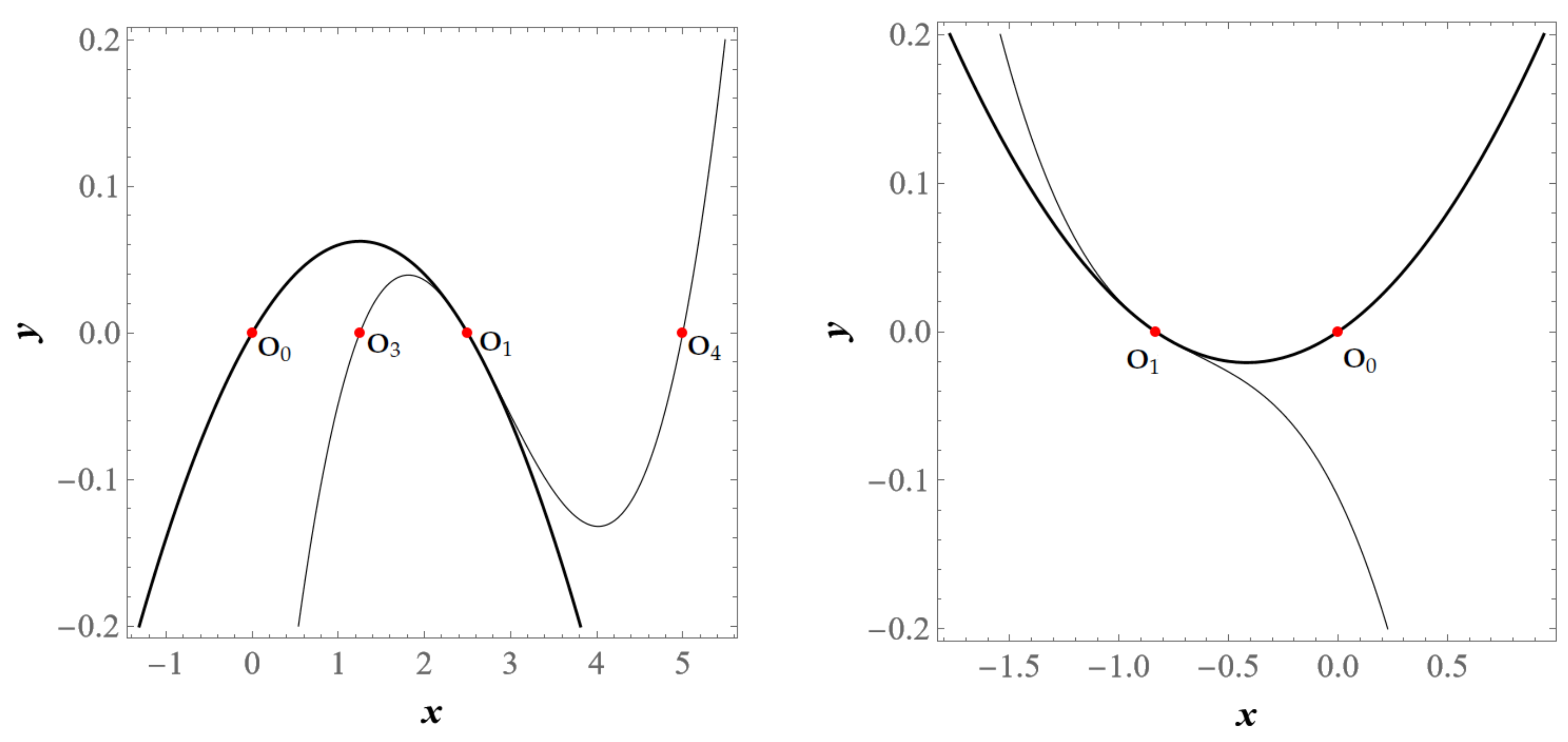
Finally, we will consider tow systems, (S1) and (S2), of the form (12) in which the parameters involved in the functions and defined by the Equations (10) and (11), respectively, are:
- (S1)
- , , , , ;
- (S2)
- , , , , .
The parameters of both systems (S1) and (S2) meet the conditions (34). Therefore, by virtue of Proposition 3 and Proposition 4, they both have second integrals and of the form (31) and (35), respectively. Consequently, the zero level sets of these second integrals provide the solution curves of the regarded systems depicted in Figure 2.
For the system (S1):
- the eigenvalues of these matrices are: and at the point , and at the point , and at the point and and at the point .
Therefore, is an unstable node, is a stable node, while and are unstable saddle points.
For the system (S2):
- the eigenvalues of these matrices are: and at the point , and and at the point .
These results allow us to conclude that is a saddle point, while is a stable node.
6. Concluding Remarks and Discussion
In this work, we have studied the nonlinear, seven-parameter, three-dimensional, cubic polynomial, autonomous differential system (1), which is proposed here as a generalization the classical [4] and recently studied [9,10,11] quadratic polynomial Hopf–Langford type systems. By introducing polar coordinates in its phase space, it has been shown that the regarded system reduces to the two-dimensional Liénard system (12), see Section 2. We have found and presented in explicit form in Section 3 polynomial first and second integrals (Darboux polynomials) of Liénard systems of the form (12). The values of the parameters for which these integrals exist have been identified.
It has been proved in Section 4 (see Theorem 1) that a generic Liénard equation is factorizable if and only if the corresponding Liénard system admits a second integral of the special form (42). It is worth noting that the factorization of Liénard type equations has been studied in a number of works (see, e.g., [21] and the references therein). However, to the best of our knowledge, here, for the first time, the factorizability of the Liénard equation has been related to the existence of second integrals (Darboux polynomials) of the corresponding Liénard system. It has been established (see Corollary 1) that each Liénard system corresponding to a Hopf–Langford system of the considered type admits a second integral of the required form (42) and hence the respective Liénard equation is factorizable.
Author Contributions
The authors made equal contributions to the elaboration of this work. Both authors have read and agreed to the published version of the manuscript.
Funding
The research that led to these results was carried out with the help of the infrastructure purchased under the National Roadmap for Scientific Infrastructure, financially coordinated by the Ministry of Education and Science of the Republic of Bulgaria (Grant No. D01-325/01.12.2023)
Data Availability Statement
Not applicable. The paper is not based on special data.
Conflicts of Interest
The author declare no conflict of interest. The funders had no role in the design of the study; in the collection, analyses, or interpretation of data; in the writing of the manuscript; or in the decision to publish the results.
References
- Hopf, E. A mathematical example displaying features of turbulence. Communications on Pure and Applied Mathematics 1948, 1, 303–322. [Google Scholar] [CrossRef]
- Ruelle, D.; Takens, F. On the nature of turbulence. Les rencontres physiciens-mathématiciens de Strasbourg-RCP25 1971, 12, 1–44. [Google Scholar]
- Hassard, B.D.; Kazarinoff, N.D.; Wan, Y.H. Theory and applications of Hopf bifurcation; Cambridge University Press: Cambridge, 1981. [Google Scholar]
- Langford, W.F. Periodic and Steady-State Mode Interactions Lead to Tori. SIAM Journal on Applied Mathematics 1979, 37, 22–48. [Google Scholar] [CrossRef]
- Nikolov, S.; Bozhkov, B. Bifurcations and chaotic behavior on the Lanford system. Chaos, Solitons & Fractals 2004, 21, 803–808. [Google Scholar] [CrossRef]
- Belozyorov, V.Y. Exponential-Algebraic Maps and Chaos in 3D Autonomous Quadratic Systems. International Journal of Bifurcation and Chaos 2015, 25, 1550048. [Google Scholar] [CrossRef]
- Yumagulov, M.G.; Fazlytdinov, M.F.; Gabdrahmanov, R.I. Langford Model: Dynamics, Bifurcations, Attractors. Lobachevskii Journal of Mathematics 2023, 44, 1953–1965. [Google Scholar] [CrossRef]
- Guo, G.; Wang, X.; Lin, X.; Wei, M. Steady-state and Hopf bifurcations in the Langford ODE and PDE systems. Nonlinear Analysis: Real World Applications 2017, 34, 343–362. [Google Scholar] [CrossRef]
- Yang, Q.; Yang, T. Complex dynamics in a generalized Langford system. Nonlinear Dynamics 2018, 91, 2241–2270. [Google Scholar] [CrossRef]
- Nikolov, S.G.; Vassilev, V.M. Assessing the Non-Linear Dynamics of a Hopf–Langford Type System. Mathematics 2021, 9, 2340. [Google Scholar] [CrossRef]
- Fu, Y.; Li, J. Bifurcations of invariant torus and knotted periodic orbits for the generalized Hopf–Langford system. Nonlinear Dynamics 2021, 106, 2097–2105. [Google Scholar] [CrossRef]
- Musafirov, E.; Grin, A.; Pranevich, A. Admissible Perturbations of a Generalized Langford System. Int. J. Bifurcat. Chaos 2022, 32. [Google Scholar] [CrossRef]
- Munteanu, F.; Grin, A.; Musafirov, E.; Pranevich, A.; Sterbeti, C. About the Jacobi Stability of a Generalized Hopf–Langford System through the Kosambi–Cartan–Chern Geometric Theory. Symmetry 2023, 15, 598. [Google Scholar] [CrossRef]
- Zhong, J.; Liang, Y. Invariant Tori and Heteroclinic Invariant Ellipsoids of a Generalized Hopf–Langford System. International Journal of Bifurcation and Chaos 2023, 33. [Google Scholar] [CrossRef]
- Liénard, A. Etude des oscillations entretenues. Revue générale de l’ électricité 1928, 23, 901–912. [Google Scholar]
- Goriely, A. Integrability and Nonintegrability of Dynamical Systems; World Scientific: Singapore, 2001. [Google Scholar]
- Kozlov, V.V. Integrability and non-integrability in Hamiltonian mechanics. Russian Mathematical Surveys 1983, 38, 1–76. [Google Scholar] [CrossRef]
- Mahomed, F.M.; Roberts, J.A.G. Characterization of Hamiltonian symmetries and their first integrals. Int. J. Non Linear Mech. 2015, 74, 84–91. [Google Scholar] [CrossRef]
- Nikolov, S.G.; Vassilev, V.M. Integrability in a nonlinear model of swing oscillatory motion. J. Geom. Symmetry Phys. 2023, 65, 93–108. [Google Scholar] [CrossRef]
- Demina, M.V. Integrability and solvability of polynomial Liénard differential systems. Studies in Applied Mathematics 2022. [Google Scholar] [CrossRef]
- González, G.; Rosu, H.C.; Cornejo-Pérez, O.; Mancas, S.C. Factorization conditions for nonlinear second-order differential equations. In Proceedings of the Nonlinear and Modern Mathematical Physics; Manukure, S., Ma, W.X., Eds.; Springer: Cham, 2024; pp. 81–99. [Google Scholar]
- Boyce, W.E.; DiPrima, R.C.; Meade, D.B. Elementary Differential Equations and Boundary Value Problems; John Wiley & Sons, Inc.: Hoboken, NJ, 2017. [Google Scholar]
Figure 1.
(Left) Phase portrait of the system of form (12) with parameters , , , , obtained by depicting a number of level sets of the corresponding first integral of the form (25). Fixed points occur at , and . (Right) Phase portrait of the system of form (12) with parameters , , , , , obtained by depicting a number of level sets of the corresponding first integral of the form (27). Fixed points occur at , and .
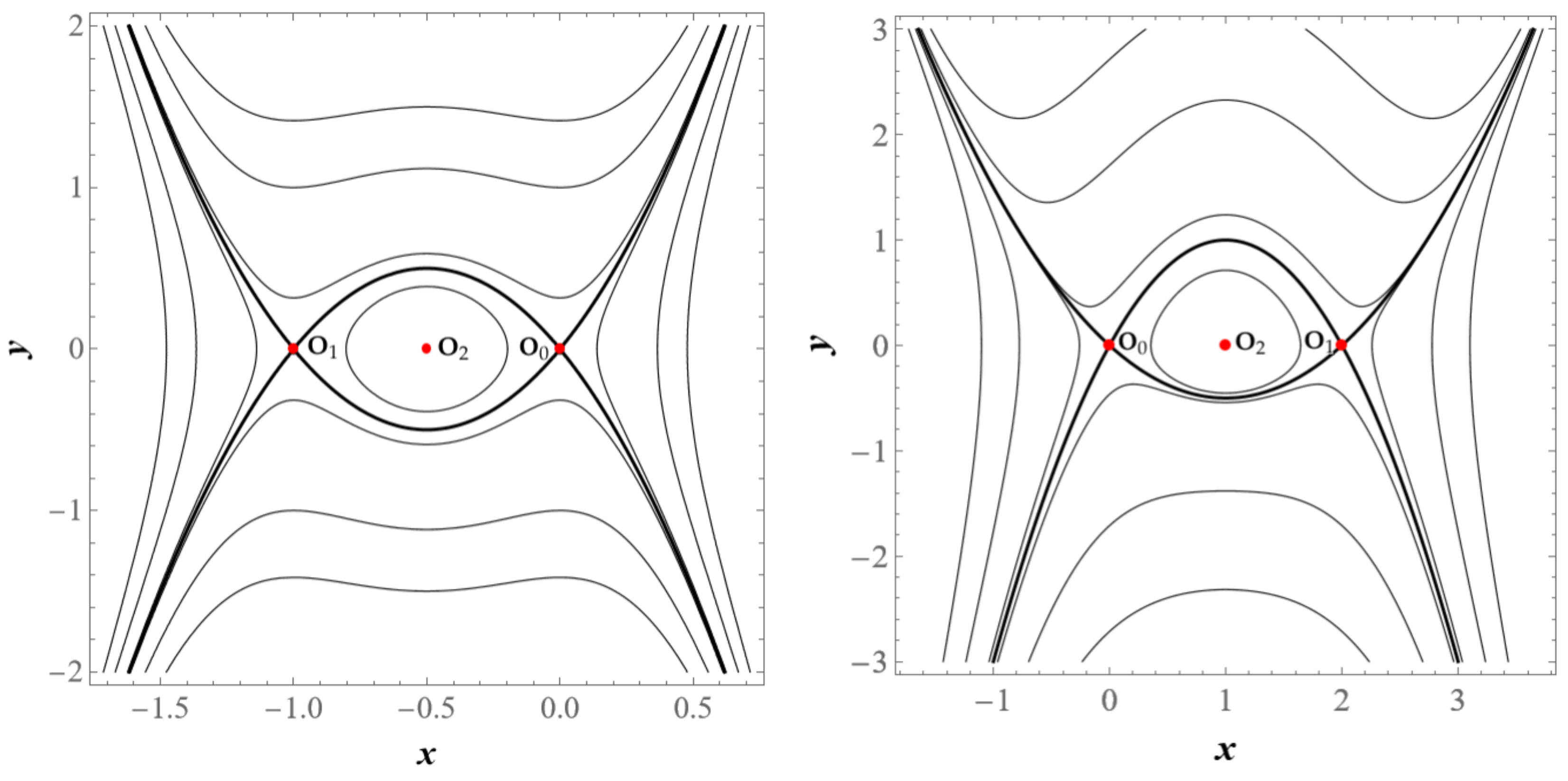
Figure 2.
(Left) Trajectories of the system of form (12) with parameters , , , , , obtained by depicting the zero level sets of the corresponding second integrals (thick curve) and (thin curve) of the form (31) and (35), respectively. Fixed points occur at , , and . (Right) Trajectories of the system of form (12) with parameters , , , , , obtained by depicting the zero level sets of the corresponding second integrals (thick curve) and (thin curve) of the form (31) and (35), respectively. Fixed points occur at and .
Disclaimer/Publisher’s Note: The statements, opinions and data contained in all publications are solely those of the individual author(s) and contributor(s) and not of MDPI and/or the editor(s). MDPI and/or the editor(s) disclaim responsibility for any injury to people or property resulting from any ideas, methods, instructions or products referred to in the content. |
© 2024 by the authors. Licensee MDPI, Basel, Switzerland. This article is an open access article distributed under the terms and conditions of the Creative Commons Attribution (CC BY) license (http://creativecommons.org/licenses/by/4.0/).
Copyright: This open access article is published under a Creative Commons CC BY 4.0 license, which permit the free download, distribution, and reuse, provided that the author and preprint are cited in any reuse.


