
Submitted:
05 November 2024
Posted:
05 November 2024
You are already at the latest version
Abstract
The paper presents a theoretical study on the dynamic behavior of a novel single-rotor system with planetary speed increaser and counter-rotating direct current (DC) generator, patented by authors, during transient stage from rest. The analytical dynamic model of the mechanical subsystem is based on the decomposition of the wind system into the component rigid bodies, followed by the description of their dynamic equations by using the Newton-Euler method. To these dynamic equations are added the linear mechanical characteristics of the DC generator and the wind rotor. The system of equations allows establishing the analytical equation of motion of the wind system and implicitly the time variation of the mechanical power parameters. Numerical simulations of the obtained analytical dynamic model were performed in MATLAB-Simulink in start-up mode from rest for the case study of a 100 kW wind turbine. These results allowed highlighting the time variation of the kinematic parameters (angular velocities and accelerations), torques and powers for all system shafts, both in transient regime and steady-state. The implementation in this case of the counter-rotating generator indicates a 6.4% contribution of the mobile stator to the generator total power. The analytical and numerical results obtained are useful to researchers, designers and developers of wind turbines aiming to optimize their construction and functionality through virtual prototyping.
Keywords:
renewable energy
; wind turbines
; counter-rotating electric generator
; dynamic modeling
; simulation
; transient regime
; steady-state
1. Introduction
Wind turbines can shutdown during operation, typically due to lack of wind, high wind speeds, or need for maintenance, and followed afterwards by the transition of the wind system from rest to operation state. The start-up of medium-large wind turbines is carried out automatically, in a controlled manner, and a priori knowledge of their dynamic behavior in transient regime represents a challenge for researchers and an advantage for designers in optimization of the control system and wind system design [1,2,3].
An important issue in approaching the wind system dynamics concerns the assumption of variable wind speed and identification of system dynamic behavior in transient regime owing to the change in wind speed or starting from rest. Dynamics studies refer both to the wind system as a whole [2,3,4,5,6,7] and to some of its component subsystems, such as electric generator [8] or mechanical gear transmission [9,10,11]: speed increaser with fixed axes [2,12], -mobile axes [7,13,14,15,16,17], or combined [18,19,20,21,22,23,24,25,26]. The overwhelming majority of these speed increasers are monomobile (single degree of freedom, 1-DOF) mechanical transmissions [2,16,19,20,23,24,25,27,28] and rarely differential transmissions [5,17]. As a result, the dynamic response of wind systems can be electrical or mechanical, depending on the type of power pursued: electrical or mechanical power, respectively.
Aiming at improving the performance of electric generators, in conjunction with their overall size reduction, various counter-rotating type generators [2,17,20,29,30] are addressed in literature: with permanent magnets [31], with liquid metals [32], respectively DFIG (Double Fed Induction Generator) that uses a back-to-back Pulse-Width converter Modulation (PWM) for bidirectional control [8].
Dynamic analysis of wind systems and their subsystems requires the use of specific software such as: FAST (Fatigue, Aerodynamics, Structures, and Turbulence) for aero-elastic dynamic modeling [33,34], MATLAB-Simulink [1,2,18,24,35,36], with results having errors below 2% compared to FAST, Ansys [15], SIMPAC [33,34] based on dynamic multibody modeling, PSCAD/EMDTC [37]. These software packages allow the identification of some representative parameters, from the operation of a wind system / subsystem in dynamic mode, related to: mechanical efficiency [2,16,38], shaft speeds [3,36,38] and torques [38,42,43], mechanical powers [3,29,38], and for electrical response: current intensity [36,38] and voltage [38].
Modeling the dynamic response of a wind system requires also knowledge of the mechanical characteristics of both the wind rotor and the electric generator. In literature, these features are modeled as nonlinear [8,27,33] or linear [2,20] functions.
In most cases, the dynamic response is an analytical or grapho-analytical result, the most common dynamic modeling methods applied for wind turbines being Newton-Euler [1,2,13,39,40,41], Lagrange+Runge-Kutta [6,22,28,42,43], lumped parameter theory [10,26,44] or polynomial chaos [12].
The dynamic behavior of a wind energy conversion system largely depends also on the moment when the electric generator is connected to the grid: either from the beginning [2,29,45], or at a time after start-up [35,36,39].
Based on this literature reviews, the following gaps emerge:
- choosing an appropriate model of the mechanical characteristics specific to the operating condition of the wind system is still a challenging issue;
- the own rotation of the satellite gears from planetary speed increasers is typically neglected;
- the choice of the optimal time for connecting the electric generator to grid.
Aiming at dealing with these gaps and deepening the understanding of the optimal functioning of a wind system, the present study focuses mainly on the following aspects:
- a)
- the dynamic modeling is carried out analytically by applying the Newton-Euler method, and the MATLAB- Simulink software in the numerical simulations;
- b)
- the considered wind system contains a wind rotor, a counter-rotating electric generator and a planetary speed increaser with one input (connected to the wind rotor) and two outputs (connected to the rotor and stator of the electric generator);
- c)
- the satellite own rotation was considered in dynamic modeling, by using an equivalent axial moment of inertia;
- d)
- the mechanical moments of inertia of the transmission components were reduced at the shafts of the wind rotor and the electric generator;
- e)
- the wind rotor mechanical characteristic is modelled by four linear zones;
- f)
- the dynamic system response is given by a simulation module that allows the connection of the generator to the grid after the wind rotor enters the maximum power characteristic. This simulator also allows the identification of the dynamic behavior of the considered subsystems through specific parameters such as: power, torque, speed and efficiency.
According to our best knowledge, there are not significant results in the literature on the generalized dynamic modeling of the mechanical system for the class of wind turbines with a single wind rotor and counter-rotating electric generator. As a result, the paper aims to cover this shortcoming by proposing an algorithm for dynamic modeling of single-rotor wind systems, which includes a counter-rotating electric generator and a speed increaser with one input and two outputs, intended to be used also in low power applications in the built environment.
The rest of the paper is organized as follows: in Section 2, the conceptual diagram and the block diagram of a wind turbine with counter-rotating generator are presented and the dynamic modeling problem is formulated; the proposed generalized algorithm, for analytical dynamic modeling, is detailed in Section 3. The numerical results obtained for the case study of a 100 kW wind turbine are presented and discussed in Section 4, and the main conclusions of the paper are drawn in Section 5.
2. Problem Formulation
Identifying the dynamic behavior of wind systems with counter-rotating generator is a challenge for designers considering the branched flow of power from the input to the two counter-rotating outputs. The generalized modeling and numerical simulation of the dynamic response of this wind turbine (WT) type is addressed in this paper. Without reducing the generality, a case study of a 1-DOF wind system is considered (Figure 1), consisting of a wind rotor R, a planetary speed increaser with one input (satellite-carrier H) and two outputs (gears 1 and 2) connected to a counter-rotating electric generator G. The rotor GR and the stator GS of the generator are both mobile and rotate in opposite directions.
The speed increaser is a planetary mechanical transmission with cylindrical gears (1–5, Figure 1), three of which are sun gears (1, 2 and 5≡0), and the solidarized gears 3 and 4 form a double satellite. In practical applications, the planetary transmission includes ns ≥ 2 equiangularly arranged double satellites (3-4).
The power input into the speed increaser (i.e., the satellite-carrier H) is solidarized with the wind rotor R. The satellites 3-4 engage on the one hand with a fixed ring gear 5, and on the other hand with the sun gear 1, connected with the generator rotor GR, and with the ring gear 2, coupled to the generator stator GS. The angular speed (ωG) of a counter-rotating generator G is given by the relative speed of the rotor GR with respect to the stator GS:
As a result, the kinematic amplification ratios, that describe the rotational speed transmission from the wind rotor to the generator rotor () and to the generator stator (), respectively, and the total amplification ratio () achieved by the wind turbine can be established through the relations:
where is the angular velocity of the body x = 1, 2, H ; – the amplification ratio from the input R to the element y = 1, 2, G.
The dynamic modeling of the analyzed 1-DOF wind system aims to identify its equation of motion , where Jx is the mechanical axial moment of inertia of the body x = 1, 2, H, and cst represents the set of other constant system parameters. The motion of the input shaft (of the wind rotor R) is considered as independent motion of the wind turbine. By solving this differential equation, the time variation of the torques and kinematic quantities (velocities and angular accelerations) related to all system shafts is obtained; the numerical simulations are performed under the assumption of starting the system from rest at a specified constant wind speed.
In the proposed dynamic modeling, the following working premises are considered:
- 1)
- The rotational elements have geometric symmetry with respect to their own axis of motion and they are rigid bodies with uniformly distributed mass; as a result, the body mass center is located on its own axis of rotation;
- 2)
- The inertial masses of the mobile elements in the planetary transmission are reduced to their outer shafts; thus, the correlations of the torques in the planetary units coincide with those of static conditions;
- 3)
- Only the gearing friction losses are considered, neglecting the friction of bearings;
- 4)
- The pitch angle of WR blades does not change during operation, therefore the adjustment parameters of the wind rotor remain constant during operation;
- 5)
- The wind rotor (input) motion is considered as independent motion of the wind system;
- 6)
- A direct current electric generator is used and, implicitly, its mechanical characteristic is a linear function with constant coefficients; in the operation of the generator, the balancing condition of the torques of the rotor GR (TGR) and of the stator GS (TGS) is described by:
- 7)
- The mechanical characteristic of the wind rotor is modeled, over its rotational speed intervals, by linear functions with constant coefficients, obviously at a constant wind speed.
Dynamic modeling of the WT mechanical system from Figure 1 is based on the block diagram depicted in Figure 2, in which the planetary speed increaser is modeled by two planetary units I (H-5-4-3-1) and II (H-5-4-3-2), connected in parallel.
Without reducing the approach generality, the simplifying case of axial moments of inertia of the bodies reduced on the outer shafts of the planetary transmission (i.e., the shafts of the R, GR and GS bodies) is considered [37]. Thus, the power transmission in dynamic mode through the speed increaser is no longer affected by the inertial properties of the component elements and, as a result, the equations of torques specific to steady-state can be used [2].
The axial moment of inertia of the ns satellites 3-4, mounted in parallel, is reduced to the satellite-carrier H axis based on the principle of equalizing kinetic energy. The satellite body has a combined rotation (around its own axis) and revolution (around the fixed sun axis) motion, its kinetic energy is considered equal to that of a virtual body with motion around the sun axis having an equivalent moment of inertia JsH:
in which
yealding to:
where ms and Js are the mass and the axial mechanical moment of a satellite 3-4, respectively (Js is established with respect to the own axis of rotation), rH is the radius of satellite axis arrangement on the carrier H, and i45 is kinematic ratio of the gear pair with fixed axes 4-5 (i.e., , where z4 and z5 are the numbers of teeth of gears 4 and 5, respectively).
Next, the main steps of the dynamic modeling algorithm are presented, based on dynamic equations of the transmission external shafts, modeled by the Newton-Euler method, the kinematic and static equations of both planetary units I and II, and the mechanical characteristics of the wind rotor and counter-rotating electric generator.
3. Dynamic Modelling
The dynamic equations of the wind system components, in the mentioned working premises, are linear differential equations of the 2nd order with constant coefficients; they can be obtained by applying the Newton-Euler method considering the positive direction of angular velocity and torque vectors according to Figure 2.
According to premise 2), the following kinematic and static equations can be written for the two planetary units PU-I and PU-II [16]:
where is the resultant torque acting on the element x; i01, i02 and η1, η2 are the internal kinematic ratio and the efficiency of PU-I and PU-II, respectively, and (see Figure 2).
The relations for the kinematic ratios and transmission efficiencies, specified in Table 1, can be easily derived from Eqs. (7).
zi is the no. of teeth of the gear i = 1...5 (see Fig. 1); η01, η02 – internal efficiency of PU-I and PU-II, respectively; η01 = η02 = , where ηg is the efficiency of a gear pair with fixed axes.
According to the block diagram in Figure 2 and Eq. (2), Table 2 illustrates the dynamic schemes of the three WT components, resulted from the decomposition of the wind system into distinctive rigid bodies, as well as their related kinematic and dynamic equations.
The set of equations in Table 2 is augmented by the linear mechanical characteristics with constant coefficients of the wind rotor (R) and generator (G):
where are constant coefficients under steady-state conditions, and by definition .
The mechanical characteristic of a wind rotor is a non-linear function [33,35], which can however be acceptably approximated by straight line segments; in this study, four-zone nonlinear characteristic modeling was adopted (Figure 3): zones I and II are used at start-up, zone III includes the point of maximum power Pmax , and zones III and IV designate the working zones of the wind rotor. Obviously, the coefficients in Eq. (8) are replace specifically by, i = 1...4 for each of these four zones I...IV.
Substituting the gear ratio and efficiency relations from Table 1 into the kinematic, static, and dynamic equations of Table 2 and corroborating with Rels. (4) and (5), the equation of motion is obtained:
This equation of motion is a nonhomogeneous second order differential equation in one variable (independent motion parameter:, where ). This differential equation is solved by numerical integration in MATLAB-Simulink, under known initial conditions: the starting from rest is considered () and the electric machine is coupled to the grid (i.e., the load is activated) when it switches to generator mode (). Knowing the time evolution of the input motion parameters, and , based on Rels. (7), (8) and Table 2, the dynamic behavior of the wind system can be determined, at start-up and in steady-state, i.e. the temporal variation of the kinematic parameters, torques and powers transmitted by all system shafts.
4. Results and Discussions
The obtained analytical dynamic model is further numerically simulated in start-up mode for the case study of a wind turbine characterized by the intrinsic geometric, kinematic and dynamic parameters centralized in Table 3. The wind turbine has a nominal power of 100 kW, generated by a rotor wind turbine with a diameter of 22.5 m at a nominal wind speed of 10.5 m/s. The start-up of the wind system is done from rest, and the electric generator load is applied at the time when . Thus, the wind system goes through three phases:
- 1)
- in the first phase, the mechanical energy generated by the wind rotor is used exclusively to overcome inertial resistance (by default, to accelerate the system),
- 2)
- in the second phase, with generator coupled to the grid, the generator resistant torque is added to the inertial load,
- 3)
- in the third phase, the wind turbine enters into steady-state (i.e., zero accelerations), obtaining the operating point described by the values of the angular velocities and torques, as well as the powers of all the shafts of the wind system, Table 4.
The results of the numerical simulation in MATLAB-Simulink, based on the equation of motion (9) and all the other equations of the analytical model, are depicted in Figure 4, Figure 5 and Figure 6. The diagrams in these figures highlight the two moments of time delimiting the three phases of the WT transition from rest to steady-state: the electric generator enters the load at ≈ 260 s, and the stabilization of the system takes place at ≈ 280 s (i.e., the starting time).
Figure 4 shows comparatively the time variations of the kinematic parameters, torques and powers from the system input vs. output. Worth noting the quasi-linear variation of all input parameters and output motions in the first part of the start-up phase 1, characterized by TG = 0 (i.e., the generator runs idle) and wind rotor operation on the zone I (see Figure 3). Since the torque generated by the wind rotor has low values at start-up (T R ≈ 2 kNm, Figure 4c), the system requires a long time (≈ 220 s) of slow increase in speed (Figure 4a) and implicitly in angular acceleration (Figure 4b) as a result of inertial resistance. Once the wind rotor enters zone II (time ≈ 220), the system is rapidly accelerated as a result of the greater torque extracted by the wind rotor from wind. The wind rotor torque reaches its maximum value at the end of the zone II (at time ≈ 255 s), followed by a torque decrease into the zone III for ≈ 5 s. At time ≈ 260 s, the electric generator enters the load (i.e. the wind system goes into the phase 2), as the operating conditions of the DC electric machine as a generator being met: (Figure 4a). The generator torque increases rapidly up to the value TG = 1.25 kNm (Figure 4c), with the decrease to zero of the angular acceleration (Figure 4b) and implicitly the entry of the system into steady-state (at time ≈ 280 s).
In phase 3, the generator power stabilizes at PG ≈ -100 kW, the mechanical power extracted from the wind being PR = 109.4 kW (Figure 4d); implicitly, the transmission efficiency has the value: . The efficiency has a value close to the value and significantly higher than (see Table 3); thus, the advantage of power branching in complex mechanisms compared to serial connection of component mechanisms in also well emphasized.
Figure 5 shows the distribution of torques and mechanical power on the inputs of planetary units I and II, as well as the inertial influence on the dynamic behavior of the wind rotor. In the first part of the phase 1 a significant difference of the driving torque TR against the resistant torque TH is noted (Figure 2 and 5a). This fact is owing to the insignificant values of the torques TH1 and TH2, also caused by the reduced inertial resistances of the output shafts (the values of the moments of inertia J1 and J2 being much lower compared to JH: J H ≈ 2000·J 1 ≈ 200·J2 , see Figure 2, Table 2 and Table 3); this reduced inertial effect of the output shafts is also confirmed by their relatively reduced values of angular accelerations. As a result, the torque TR is mostly used to overcome the inertial load of the input shaft H. Once the generator enters the load, the TH1 torque increases much faster than TH2, becoming the major component of TH in steady-state. Although the GR rotor and GS stator torques are equal in steady-state, the significant difference between TH1 and TH 2 is explained by the large differences in the amplification ratios and (see Table 3), corresponding to the two power branches. The power variation on the input shafts (Figure 5b) follows a similar evolution as the input torques (Figure 5a): most of the wind rotor power (over 93%) is directed to the planetary unit I and, implicitly, to the GR rotor - the body with the highest rotation speed.
Figure 6 illustrates the WT dynamic behavior at output side, characterized by the branched power transmission via the rotor GR and the stator GS, respectively; the contribution of the mobile stator to the overall performance of the wind system is particularly highlighted. The output angular speeds and accelerations (Figure 6a,b) have a linear dependence on the independent motion of the wind rotor; according to the relations in Table 2, they follow the variation profile of the angular velocity ωRand acceleration εR, respectively (Figure 4a,b), with values amplified with the ratios ia1, ia2 and iaG, respectively. Note the much lower speed and acceleration of the GS stator compared to the GR rotor, and finally the smaller power contribution from the GS stator vs. GR rotor due to the large inequality: ǀia2ǀ << ia1. Obviously, this situation can be improved by optimizing the ratio between ia2 and ia1, as well as the large ratio between the inertia of the GS stator and the GR rotor.
At the time the generator enters the load (≈ 260 s), the torques T1 (Figure 6c) and T2 (Figure 6e), respectively the powers P1 (Figure 6d) and P2 (Figure 6f) reflect the inertial impact of the output shafts (1 and 2). Although the two shafts have different moments of inertia (J2 = 10J1 , see Table 3), the large acceleration difference in favor of shaft 1 ≡ GR makes the inertial resistance of shaft 1 greater than that of shaft 2 (maximum 0.172 vs. 0.118 kNm) in phase (1). In steady-state, the high angular velocity of the GR rotor allows it to receive a much higher power compared to the GS stator (i.e., ǀPGRǀ = 93.34 kW > ǀPGSǀ = 6.40 kW). Thus, the power contribution of the GS stator to the total power of the generator is ~ 6.4% (Figure 6g), the largest share of the power flow being distributed to the GR rotor.
The results of the dynamic numerical simulations, based on the analytical dynamic model developed in this study, allow the identification of the WT dynamic behavior in transient regime, during starting-up from rest, as well as the values of the operating point parameters in steady-state.
5. Conclusions
The paper presents a generalized dynamic modeling approach of a 1-DOF single-rotor wind system with planetary speed increaser and counter-rotating DC generator, characterized by power flow branching at the mechanical transmission output. In the proposed dynamic modeling algorithm, the dynamic equations of the system shafts, the mechanical characteristics of the wind rotor and of the electric generator are considered, to which the kinematic and static equations of the planetary units I and II are added. This system of equations allows the analytical establishment of the wind system equation of motion and implicitly its operating point by numerical solution in transient mode and in steady-state.
The analytical study and the results of the numerical simulations, carried out on a case study of a wind turbine with rated power of 100 kW, allowed to draw the following conclusions:
- the proposed generalized modeling algorithm allows obtaining analytically the equation of motion of the wind system, formulated as a nonhomogeneous differential equation of the second order in a single independent variable, describing the wind rotor motion;
- by numerically solving the equation of motion, using the MATLAB- Simulink software, the dynamic response of the wind system in transient mode and as well the operating point in steady-state are obtained;
- the analysis of the dynamic response in transient mode, when starting from rest at constant wind speed, allowed the identification of the starting time of the wind system, as well as the stresses induced by the inertial load alone and by its combination with the generator load;
- unlike the case of traditional wind turbines, equipped with conventional generator with fixed stator, the counter-rotating generator allows an additional input of power brought by the mobile stator GS; in the analyzed case, the additional power supply by GS in steady-state is ~ 6.4%.
The proposed generalized algorithm can be applied, with rigorous adaptations, to other types of wind systems, regardless of their complexity: with one or more wind rotors, with conventional or counter-rotating electric generator, with fixed-axis or planetary speed increaser. Likewise, the developed MATLAB-Simulink model can also be applied iteratively for the purpose of constructive-functional optimization of this particular type of wind system, as well as in the simulation scenarios of variable operational conditions determined by the change in wind speed
The authors intend to address in the future the dynamic optimization of such wind system and the validation of theoretical results through the experimental research of some functional models on specialized testing rigs.
Patents: Saulescu, R., Neagoe, M., Visa, M., Jaliu, C., Munteanu, O., Totu, I. Cretescu, N. Monomobile planetary speed increaser with two counter-rotating outputs, Patent no RO 131740 B1, 11/29/2023.
Author Contributions
Conceptualization, M.N. and R.S.; methodology, M.N. and R.S.; software, R.S. and M.N.; validation, M.N. and R.S.; formal analysis, M.N. and R.S.; investigation, R.S. and M.N.; resources, R.S. and M.N.; data curation, M.N. and R.S.; writing—original draft preparation, M.N. and R.S.; writing—review and editing, M.N.; visualization, R.S.; supervision, M.N. All authors have read and agreed to the published version of the manuscript.
Funding
This research received no external funding.
Institutional Review Board Statement
Not applicable.
Informed Consent Statement
Not applicable.
Data Availability Statement
Not applicable.
Acknowledgments
Not applicable.
Conflicts of Interest
The authors declare no conflict of interest.
References
- Cottura, L. Caradonna, R., Ghigo, A., Novo, R., Bracco, G., Mattiazzo G. Dynamic Modeling of an Offshore Floating Wind Turbine for Application in the Mediterranean Sea. Energies 2021, 14, 248. [Google Scholar] [CrossRef]
- Neagoe, M. , Saulescu, R., Jaliu, C., Neagoe, I. Dynamic Analysis of a Single-Rotor Wind Turbine with Counter-Rotating Electric Generator under Variable Wind Speed. Appl. Sci. 2021, 11, 8834. [Google Scholar] [CrossRef]
- Sanchez, R. , Medina, A. Wind turbine model simulation: A bond graph approach. Simulation Modelling Practice and Theory 2014, 41, 28–45. [Google Scholar] [CrossRef]
- Al-Hamadani, H. , An, T., King, M., Long, H. System Dynamic Modelling of Three Different Wind Turbine Gearbox Designs under Transient Loading Conditions. International Journal of Precision Engineering and Manufacturing 2017, 18, 11. [Google Scholar] [CrossRef]
- Lin, A.-D.; Hung, T.-P.; Kuang, J.-H.; Tsai, H.-A. Power Flow Analysis on the Dual Input Transmission Mechanism of Small Wind Turbine Systems. Appl. Sci. 2020, 10, 7333. [Google Scholar] [CrossRef]
- Rubio, J.J. , Soriano, L.A., Yu, W. Dynamic Model of a Wind Turbine for the Electric Energy Generation. Dynamic Model of a Wind Turbine for the Electric Energy Generation. Mathematical Problems in Engineering 2014. [CrossRef]
- Wang, B. , Michon, M., Holehouse, R., Atallah, K. Dynamic Behaviour of a Multi-MW Wind Turbine. 2015. 978-1-4673-7151-3/15/$31.00 IEEE.
- Abo-Khalil, A. , Alyami, S., Sayed K., Alhejji A. Dynamic Modeling of Wind Turbines Based on Estimated Wind Speed under Turbulent Conditions. Energy 2019, 12, 1907. [Google Scholar] [CrossRef]
- Dewangan, P. , Parey, A., Hammami, A., Chaari F., Haddar, M. Dynamic characteristics of a wind turbine gearbox with amplitude modulation and gravity effect: Theoretical and experimental investigation. Mechanism and Machine Theory 2022, 167, 104468. [Google Scholar] [CrossRef]
- Dong, H. , Zhang, C., Wang, D., Xu, S. Dynamic characteristics of gear box with PGT for wind turbine. Dynamic characteristics of gear box with PGT for wind turbine. Procedia Comput. Sci. 2017, 109. [Google Scholar] [CrossRef]
- Fan, Z. , Zhu, C., Li, X., Liang, C. The transmission characteristic for the improved wind turbine gearbox. Energy Sci. Eng. 2019, 7, 1368–1378. [Google Scholar] [CrossRef]
- Mabrouk, I.B. , Hami, A.E., Walha, L., Zghal, B., Haddar, M. Dynamic response analysis of Vertical Axis Wind Turbine geared transmission system with uncertainty. Dynamic response analysis of Vertical Axis Wind Turbine geared transmission system with uncertainty. Engineering Structures 2017, 139. [Google Scholar] [CrossRef]
- Li, D. , Zhao, Y. A dynamic-model-based fault diagnosis method for a wind turbine planetary gearbox using a deep learning network. Protection and Control of Modern Power Systems. [CrossRef]
- Mathis, R. , Rémond, Y. Kinematic and dynamic simulation of epicyclic gear trains. Mech. Mach. Theory 2009, 44, 412–424. [Google Scholar] [CrossRef]
- Mohsine, A. , Mostapha,B.E., Alaoui, R.E., Daoudi, K. Comparative Study in the Structural and Modal Analysis of a Wind Turbine Planetary Gear Based on Material Reduction Criteria Using FEM. International Journal of Renewable Energy Research 2019, 9, 2. [Google Scholar] [CrossRef]
- Neagoe, M. , Saulescu, R., Jaliu, C. Simionescu, P.A. A Generalized Approach to the Steady-State Efficiency Analysis of Torque-Adding Transmissions Used in Renewable Energy Systems. Energies 2020, 13, 4568. [Google Scholar] [CrossRef]
- Saulescu, R. , Neagoe, M., Jaliu, C., Munteanu, O. A Comparative Performance Analysis of Counter-Rotating Dual-Rotor Wind Turbines with Speed-Adding Increasers. Energies 2021, 14, 2594. [Google Scholar] [CrossRef]
- Girsang, I,P., DhupiaS.J., Muljadi, E., Singh, M., Pao, Y.P. Gearbox and Drivetrain Models to Study Dynamic Effects of Modern Wind Turbines. IEEE Transactions on Industry Applications 2013, 50 (6). [CrossRef]
- Li, Z. , Wen, B., Peng, Z., Dong, X., Qu, Y. Dynamic modeling and analysis of wind turbine drivetrain considering the effects of non-torque loads. Applied Mathematical Modelling 2020, 83, 146–168. [Google Scholar] [CrossRef]
- Neagoe, M. , Saulescu, R., Jaliu, C. Design and Simulation of a 1 DOF Planetary Speed Increaser for Counter-Rotating Wind Turbines with Counter-Rotating Electric Generators. Energies 2019, 12, 1754. [Google Scholar] [CrossRef]
- Nejad, A.R. , Guo, Y., Gao, Z., Moan, T. Development of a 5 MW Reference Gearbox for Offshore Wind Turbines. Wind Energy 2016, 9, 6. [Google Scholar] [CrossRef]
- Ren, Z. , Zhou, S., Wen, B. Dynamic coupled vibration analysis of a large wind turbine gearbox transmission system. Journal of Vibroengineering 2015, 7, 6. [Google Scholar]
- Shi, W. Kim, C.-W., Chung, C.-W., Park, H.-C. Dynamic Modeling and Analysis of a Wind Turbine Drivetrain Using the Torsional Dynamic Model. Int. J. Precis. Eng. Manuf 2012, 14, 153–159. [Google Scholar] [CrossRef]
- Shi, W. , Ning, D., Ma, Z., Ren, N., Park H. Parametric Study of Drivetrain Dynamics of a Wind Turbine Using the Multibody Dynamics. International Journal of Mechanical Engineering and Applications 2019, 7, 2. [Google Scholar] [CrossRef]
- Shi, W. , Park, H.-C., Na, S., Song, J., Ma, S., Kim, C.-W. Dynamic Analysis of Three-Dimensional Drivetrain System of Wind Turbine. International Journal of Precision Engineering and Manufacturing 2014, 15, 7. [Google Scholar] [CrossRef]
- Wang, J. , Yang, S., Liu, Y., Mo, R. Analysis of Load-Sharing Behavior of the Multistage Planetary Gear Train Used in Wind Generators: Effects of Random Wind Load. Appl. Sci. 2019, 9, 5501. [Google Scholar] [CrossRef]
- Farias, M.G. , Galhardo, A.B.M., Vaz, R.P.J., Pinho, T.J. A steady-state based model applied to small wind turbines. Journal of the Brazilian Society of Mechanical Sciences and Engineering. [CrossRef]
- Xiang, L. , Gao, N., Hu, A. Dynamic analysis of a planetary gear system with multiple nonlinear parameters. Dynamic analysis of a planetary gear system with multiple nonlinear parameters. J. Comput. Appl. Math. 2017, 327. [Google Scholar] [CrossRef]
- Erturk, E. , Sivrioglu, S., Bolat, F.C. Analysis Model of a Small Scale Counter-Rotating Dual Rotor Wind Turbine with Double Rotational Generator Armature. International Journal of Renewable Energy Research 2018, 8, 4. [Google Scholar] [CrossRef]
- Wrobel, R. , Drury, D., Mellor, P.D., Booker, J.D. Contra-Rotating Modular Wound Permanent Magnet Generator for a Wind Turbine. 4th IET Conference on Power Electronics, Machines and Drives 2008, 330-334. [CrossRef]
- Booker, J.D. , Mellor, P.H., Wrobel, R., Drury D. A compact, high efficiency contra-rotating generator suitable for wind turbines in the urban environment. Renew. Energy 2010, 35, 2027–2033. [Google Scholar] [CrossRef]
- Egorov, A.V., Kaizer, Y.F., Lysyannikov, A.V., Kuznetsov, A.V., Shram, V.G., Pavlov, A.I., Smirnov, M.Y., Kuznetsova, P.A. Counter-rotating electric generator for wind power plants with liquid metal energy transfer. Journal of Physics: Conference Series 2021, 2094 052018. [CrossRef]
- Dong, W. , Xing, Y., Moan, T. Time Domain Modeling and Analysis of Dynamic Gear Contact Force in a Wind Turbine Gearbox with Respect to Fatigue Assessment. Energies 2012, 5, 4350–4371. [Google Scholar] [CrossRef]
- Xing, Y. , Guo, Y., Keller, J., Moan, T. Model Fidelity Study of Dynamic Transient Loads in a Wind Turbine Gearbox. WINDPOWER Conference 2013. https://www.osti.gov/biblio/1078065.
- Jansuya, P. , Kumsuwan, Y. Design of MATLAB/Simulink Modeling of Fixed-pitch Angle Wind Turbine Simulator. Energy Procedia 2013, 34, 362–370. [Google Scholar] [CrossRef]
- Oyekola, P. , Mohamed, A., Pumwa, J. Renewable Energy: Dynamic Modelling of a Wind Turbine. Int. J. Innov. Technol. Explor. Eng. 2019, 9, 9. [Google Scholar] [CrossRef]
- Santoso, S. , Le, H. Fundamental time–domain wind turbine models for wind power studies. Renew. Energy 2007, 32, 2436–2452. [Google Scholar] [CrossRef]
- Teixeira, M.R. , Ohara, M. F., Milhomens, D. M., de Paula S. A. Dynamical Behavior of a Wind Turbine Power Train Considering a Rotor-Gearbox-Generator Coupled Model. Eccomas Proceedia COMPDYN, 3555. [Google Scholar] [CrossRef]
- Fernández, M.L. Saenz, J.R., Jurado, F. Dynamic models of wind farms with fixed speed wind turbines. Renew. Energy 2006, 31, 1203–1230. [Google Scholar] [CrossRef]
- Song, Z. , Shi, T., Xia, C., Chen, W. A novel adaptive control scheme for dynamic performance improvement of DFIG-Based wind turbines. Energy. [CrossRef]
- Zhao, M. , Ji, J. Dynamic Analysis of Wind Turbine Gearbox Components. Energies 2016, 9, 110. [Google Scholar] [CrossRef]
- Park, Y. , Shi, W., Park, H. Effect of the Variable Gear Mesh Model in Dynamic Simulation of a Drive Train in the Wind Turbine. Effect of the Variable Gear Mesh Model in Dynamic Simulation of a Drive Train in the Wind Turbine. Engineering Review 2020, 113–124. [Google Scholar] [CrossRef]
- Park, Y. Park, H., Ma, Z., You, J., Shi, W. Multibody Dynamic Analysis of a Wind Turbine Drivetrain in Consideration of the Shaft Bending Effect and a Variable Gear Mesh Including Eccentricity and Nacelle Movement. Frontiers in Energy Research 2021, 8, 604414. [Google Scholar] [CrossRef]
- Zhu, C. , Xu, X., Liu, H., Luo, T., Zhai, H. Research on dynamical characteristics of wind turbine gearboxes with flexible pins. Research on dynamical characteristics of wind turbine gearboxes with flexible pins. Renew. Energy 2014, 68. [Google Scholar] [CrossRef]
- Yi, P. , Zhang, C., Guo, L., Shi, T. Dynamic modeling and analysis of load sharing characteristics of wind turbine gearbox. Advances in Mechanical Engineering 2015, 7, 3. [Google Scholar] [CrossRef]
Figure 1.
Conceptual scheme of the single-rotor wind turbine with counter-rotating electric generator.
Figure 1.
Conceptual scheme of the single-rotor wind turbine with counter-rotating electric generator.
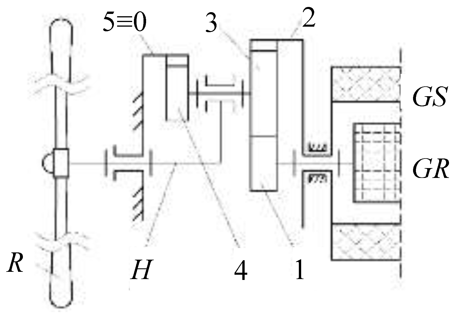
Figure 2.
Block scheme of the single-rotor wind turbine with counter-rotating electric generator.
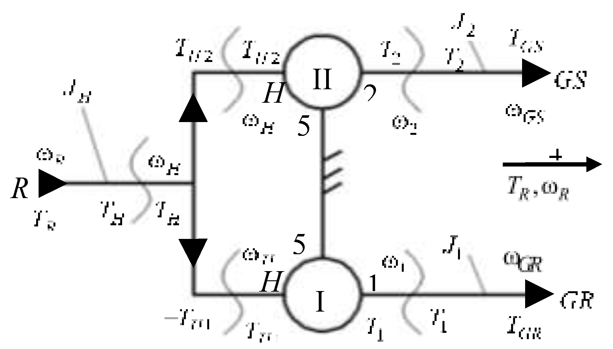
Figure 3.
The mechanical characteristic of a wind rotor modeled by four linearized zones.
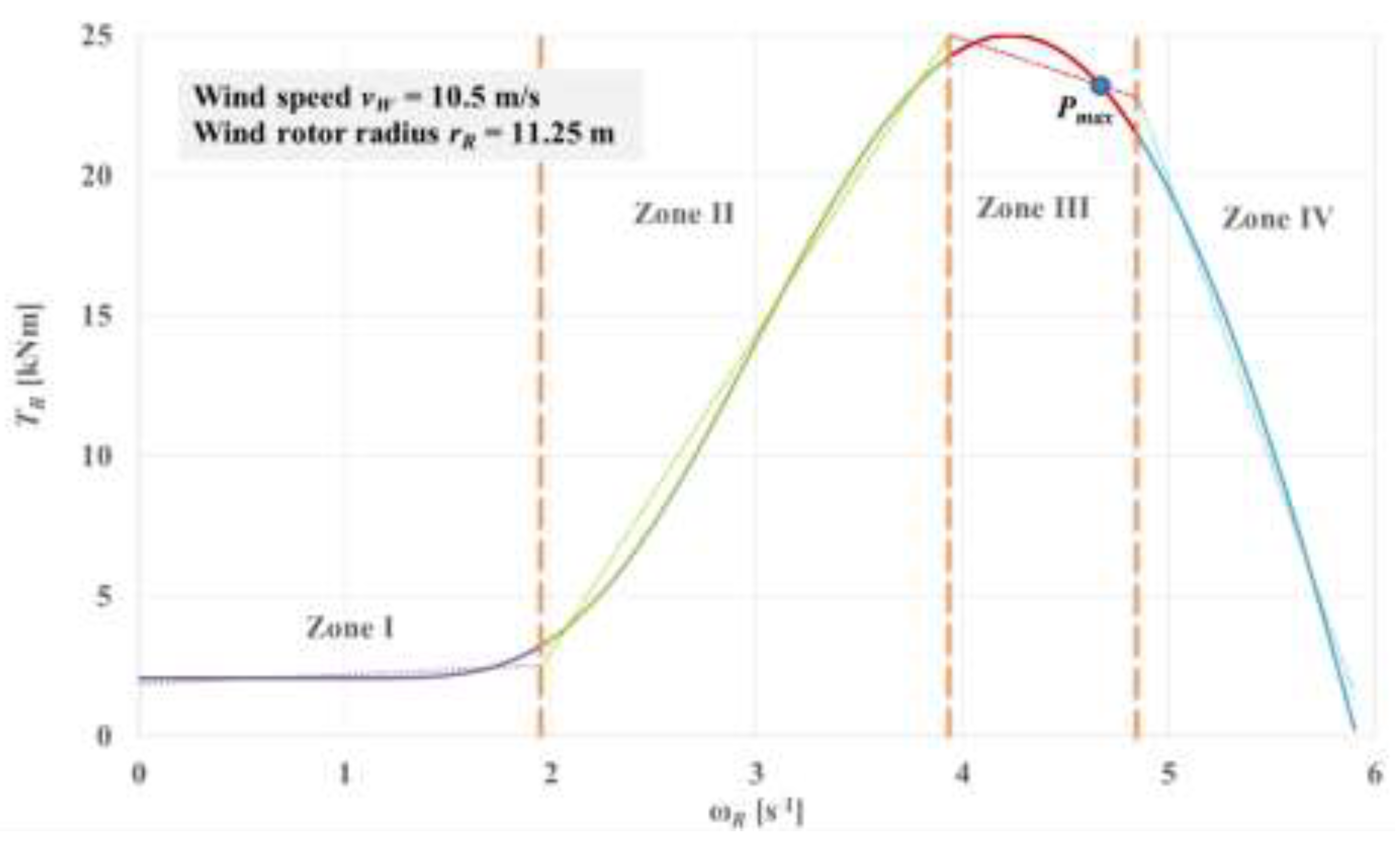
Figure 4.
The wind system dynamic response: (a) input vs. output angular speeds; (b) input vs. output angular accelerations; (c) wind rotor vs. generator torques; (d) wind rotor vs. generator powers.
Figure 4.
The wind system dynamic response: (a) input vs. output angular speeds; (b) input vs. output angular accelerations; (c) wind rotor vs. generator torques; (d) wind rotor vs. generator powers.
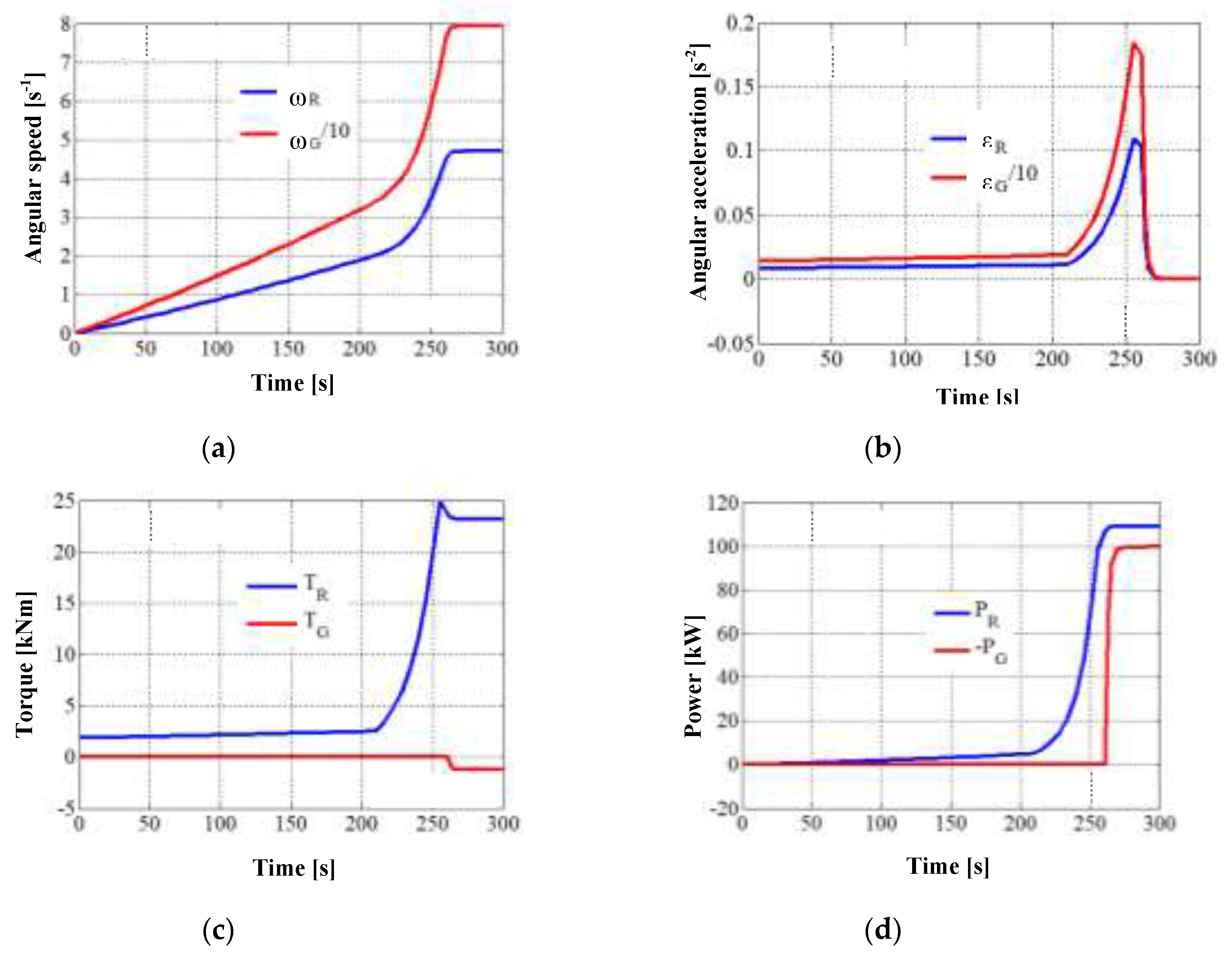
Figure 5.
The dynamic response at wind rotor side: (a) wind rotor vs. input torques; (b) wind rotor vs. input powers.
Figure 5.
The dynamic response at wind rotor side: (a) wind rotor vs. input torques; (b) wind rotor vs. input powers.
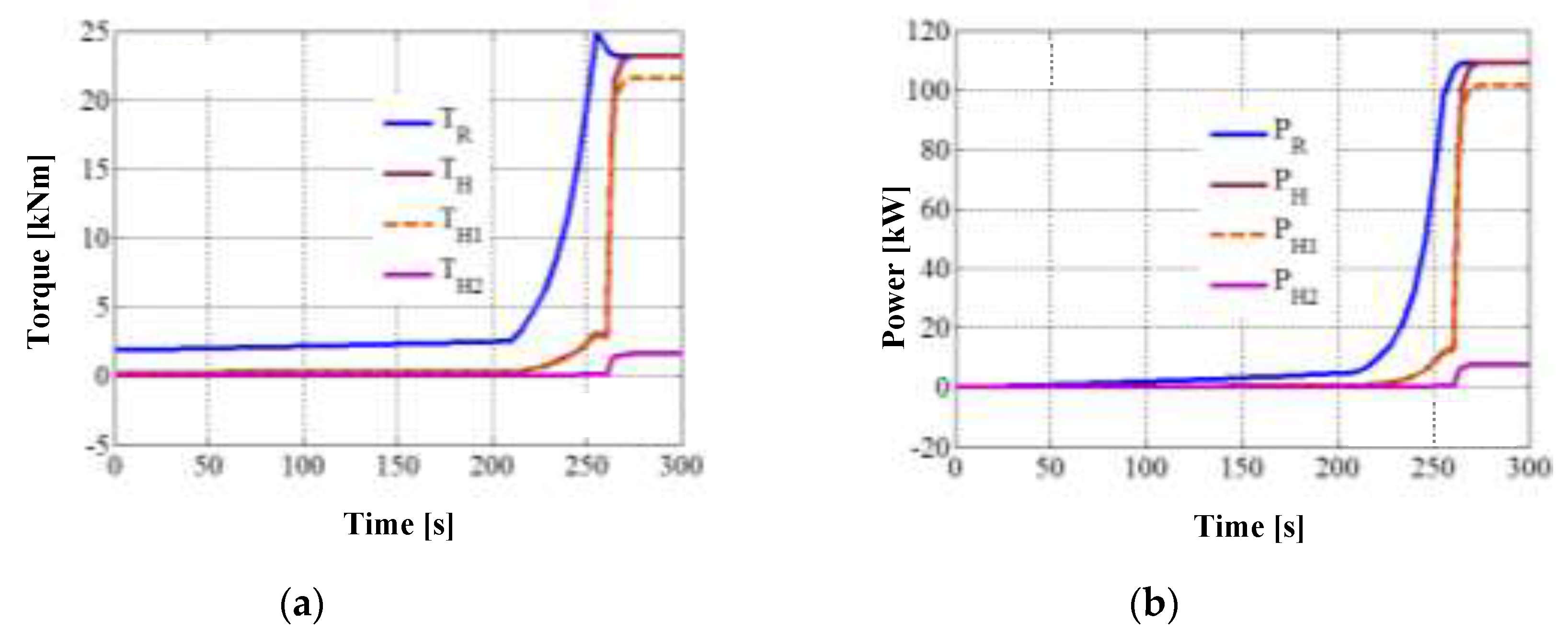
Figure 6.
The dynamic response at generator side: (a) generator angular speeds; (b) generator angular accelerations; (c) generator rotor vs. output 1 torques; (d) generator rotor vs. output 1 powers; (e) generator stator vs. output 2 torques; (f) generator stator vs. output 2 powers; (g) mechanical powers.
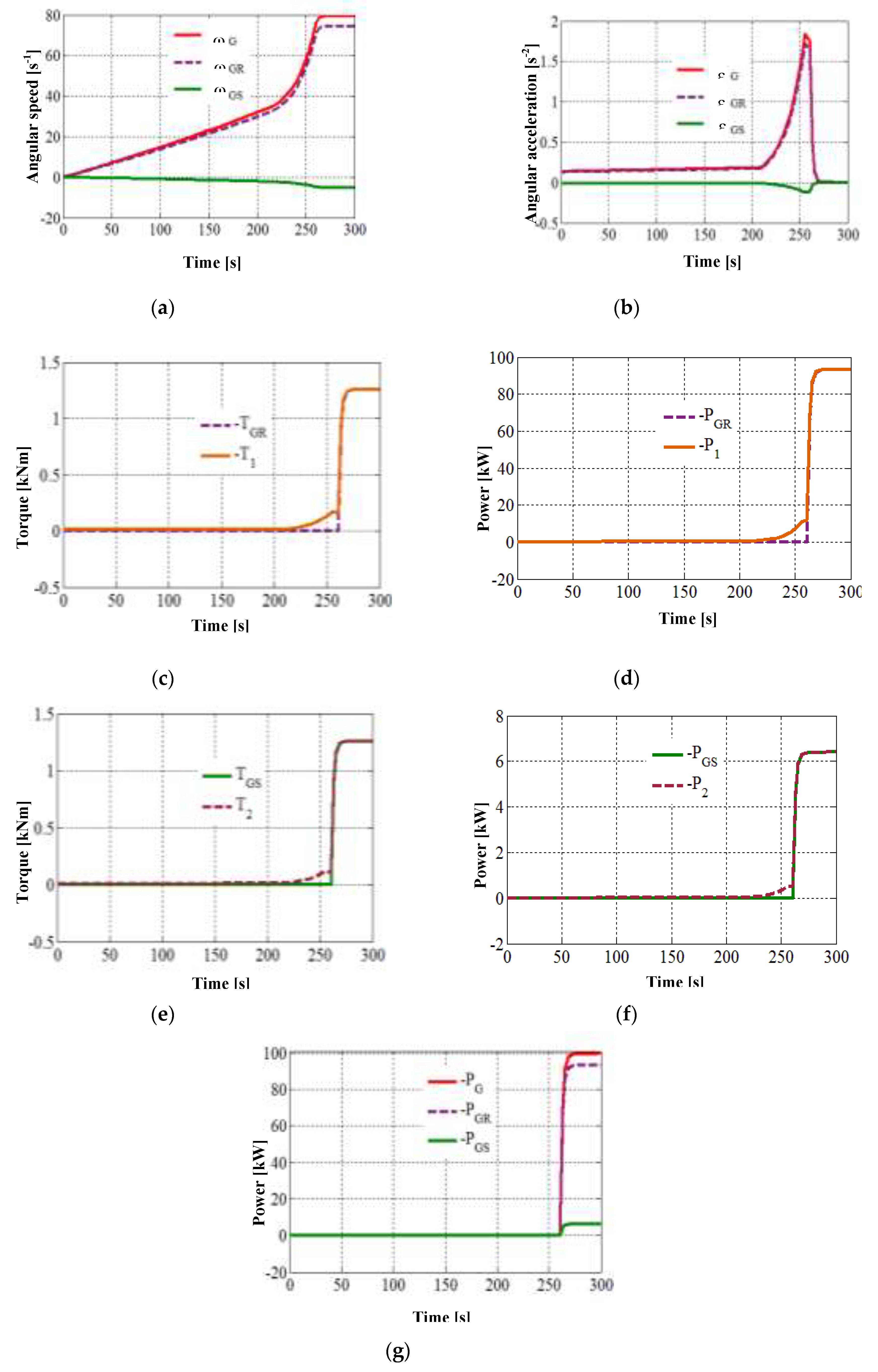

Table 1.
Transmission ratios and efficiencies.
| PU | |||
|---|---|---|---|
| I | |||
| II |
Table 2.
Schemes and dynamic equations of the WT components.
| Body | Dynamic schemes | Equations |
|---|---|---|
 | ||
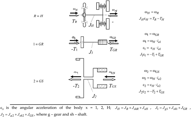 | ||
Table 3.
Constant intrinsic parameters of the wind system.
| zi | a [kNms] b [kNm] |
J [kgm2] | |||
|---|---|---|---|---|---|
Table 4.
Operating point of the wind system in steady-state.
| Shaft | Torque [kNm] |
Angular speed [s -1] |
Power [kW] |
|---|---|---|---|
| R ≡ H | 23,208 | 4,704 | 109.17 |
| H 1 | 21,600 | 4,704 | 101.61 |
| H 2 | 1,608 | 4,704 | 7.56 |
| 1 ≡ GR | -1,256 | 74,317 | -93.34 |
| 2 ≡ GS | 1,256 | -5,097 | -6.40 |
| G | -1,256 | 79,414 | -99.75 |
Disclaimer/Publisher’s Note: The statements, opinions and data contained in all publications are solely those of the individual author(s) and contributor(s) and not of MDPI and/or the editor(s). MDPI and/or the editor(s) disclaim responsibility for any injury to people or property resulting from any ideas, methods, instructions or products referred to in the content. |
© 2024 by the authors. Licensee MDPI, Basel, Switzerland. This article is an open access article distributed under the terms and conditions of the Creative Commons Attribution (CC BY) license (http://creativecommons.org/licenses/by/4.0/).
Copyright: This open access article is published under a Creative Commons CC BY 4.0 license, which permit the free download, distribution, and reuse, provided that the author and preprint are cited in any reuse.


