Submitted:
18 October 2024
Posted:
22 October 2024
You are already at the latest version
Abstract
In this study, the asymmetric effect of oil and natural gas price shocks on the trade balance of 11 CESEE countries was estimated. These countries are net importers of oil and natural gas, and price shocks are often the cause of imbalances in trade. Quarterly data for the period 1994Q1 to 2023Q4 and nonlinear ARDL model were used. In the long run, a significant asymmetric effect due to the oil price shock on the trade balance of Bulgaria, Czechia, Latvia and Slovenia was found, as well as a significant asymmetric effect due to the natural gas price shock on the trade balance of Croatia. Also in the long run, a significant asymmetric effect due to wholesale prices on the trade balance of Romania, Bulgaria and Croatia was found as well as a significant asymmetric effect due to industrial production on the trade balance of Croatia, Czechia and Latvia was found, in addition to a significant asymmetric effect due to the exchange rate on the trade balance of Czechia, Poland and Romania.
Keywords:
oil
; natural gas
; price shock
; trade balances
; asymmetry
1. Introduction
Oil price shocks cause global economic crises that have different effects on oil importing and exporting countries. The first oil shock of 1973-74 and the second oil shock of 1979-80 caused the oil prices to reach a historic maximum, and this called into question the macroeconomic balance of the majority of the oil importing countries. The financial crisis of 2008 and the Russia-Ukraine war that started in 2022 have had similar effects, causing an energy crisis leading to a rise in oil prices, in particular the rise in natural gas prices.
Oil and natural gas are considered essential industrial inputs and any significant change in their price is reflected in macroeconomic variables such as growth, exchange rate, inflation, consumption and trade balance, etc. (1, 2, 3, 4, 5,). Over the last five decades, the world has seen a global rise in oil imports as a result of the growth of the world economy and increased consumption, while a growth of natural gas imports has been seen due to a greater share of gas in the industrial production and the Russian-Ukraine war.
The subject of this study refers to estimating the effect of oil and natural gas price shocks on the trade balance of 11 CESEE countries. In the past, these countries belonged to the socialist bloc and inherited the problem of a trade deficit and high dependency on the importing of oil and natural gas (6). Also, over recent decades, these countries have achieved significant economic progress and are currently classified as the fastest growing economies with significant potential. The economic growth of these countries has brought about a greater demand for and consumption of oil and natural gas. Therefore, one of the principal motives of this study is to examine whether the oil and natural gas price shocks are the cause of instability in the CESEE countries’ trade balance.
The existing studies, done for the Central and Eastern European (CIE) countries, have mostly examined the effect of oil price shocks on economic growth, current account deficit, share price and the exchange rate. The existing studies lack the estimation of the relationship between oil and natural gas price shocks and the total trade balance. The authors of the study deem that the estimate of the effect of oil and natural gas price shocks on the total balance of trade is significant as it explains to what extent the price shocks have an effect on trade balance. In addition, the existing studies noted there to be symmetry between the oil price shock and trade balance or economic growth. An increase in oil price leads to a trade deficit, while a decrease in oil price leads to a decrease in trade deficit. Due to structural shocks, external shocks, financial crises and trade reforms, there are often shocks to the global oil market which cause an increase or decrease in price. An increase or decrease in oil price has no effect on the trade balance in developed countries that import oil because they have surplus of non-oil trade balance which exceeds the deficit of the oil trade balance. Likewise, a decrease in oil price on the global market does not have a positive effect on the trade balance of the emerging economies that are oil importers. In that sense, this study is different compared to the existing studies as it examines the asymmetric relation between oil price shocks and trade balance. Also, this study will additionally differ from the existing studies in that it will examine, in addition to the effect of oil price shocks, also natural gas price shocks on trade balance which has not been sufficiently looked into. One of the possible explanations as to why the effect of natural gas price shocks on trade balance has not been examined so far may be that natural gas is considered to be an oil by-product and that any increase in the price of oil has an effect on the increase of the price of gas (7). However, in production industries, oil and natural gas are seen as different inputs. The energy price responds more strongly to oil price shocks, while the basic prices of products respond more strongly to natural gas price shocks, since gas is used more in the production of basic products.
The objective of this study is to estimate the non-linear effect of oil and natural gas price shocks on the trade balance of 11 CESEE countries (Bulgaria, Estonia, Croatia, Latvia, Lithuania, Czechia, Hungary, Poland, Romania, Slovakia and Slovenia). We used Shin et al. (8) the nonlinear autoregressive distributed lag (NARDL) model and quarterly data for the period 1994Q1 to 2023Q4 (9,10).
This study will fill the gap in the existing literature that has not examined the asymmetric effect of oil and natural gas price shocks on the trade balance of CESEE countries. Namely, up until the mid-1980s, linear models claimed that there was symmetry between the price of oil and economic growth. Namely, during the 1980s, a decrease in the price of oil did not have a significant effect on economic growth. This undermined the reliability of linear models and was the reason for economists such as Hamilton (4) applying non-linear models (11). The asymmetric or non-linear models showed that the rise in oil price has a different effect than a drop in oil price on trade balance or economic growth, which is in opposition to symmetric models that deem that a rise and drop in oil prices has a linear effect. Accordingly, Shin et al. (8) non-linear ARDL model was used to carry out an assessment of the positive and negative partial sum decompositions and the identification of the asymmetric effect in the short and long run. The presence of asymmetry involves different responses by the trade balance to increase and decrease the oil and natural gas prices (10).
This study is structured as follows. In section two, a literature review is presented. In section three, the methodology is presented. Section four presents the results, and section five presents the conclusions.
2. Literature review
In this section, the existing literature that explains the effect of oil and natural gas price shocks on the trade balance of the countries importing and exporting oil will be presented (Table 1). Allegret et al. (12) found that a rise in oil price has a positive effect on the trade balance of the exporting countries. The transmission of oil price through the trade channels has a negative effect on the balance of the world trade. Similarly, Alkhateeb and Mahmood (13) and Nasir et al. (14) found asymmetry for the Gulf countries (Kuwait, UAE, Oman and S. Arabia) and it was noted that oil price rise has a positive effect on the trade balance, while an oil price drop has a negative effect on the trade balance of Bahrein. Contrary to this, in oil importing countries, Huntington (15), Kilian et al. (16), and Moshiri and Kheirandish (17) found in particular those less developed among them, an oil price rise has a negative effect on their trade balance. For rich oil importing countries, an oil price rise does not have negative effect on the trade balance in the long run because their non-oil trade balance is in surplus. Similarly, Korhonen and Ledyaeva (18) found that oil shock supply has a negative effect on the decrease in imports, and that it causes a deficit of trade balance for the countries importing and exporting oil. The oil shock demand also leads to growth in oil price and inflation. As a result, growth and the demand for oil in the importing countries decreases, which indirectly has a negative effect on their trade balance. Contrary to this, Taghizadeh-Hesary et al. (19) used a large sample of oil importing and exporting countries and found that shock demand has a positive effect on the exports and trade balance of the oil exporting countries, while shock supply has a negative effect on the oil trade balance of the oil importing countries. However, all oil importing countries have a greater non-oil surplus in trade balance than they do an oil deficit in trade balance, ensuring a positive total trade balance for these countries. Contrary to this, Bodenstein et al. (20) found that due to incomplete financial markets in oil importing countries, one sees the transfer of wealth going towards the oil exporting countries. Despite the growth of the oil deficit in the trade balance of importing countries, these countries achieve balanced trade due to having a non-oil surplus in their trade balance. On the one hand, Rafiq et al. (5) found that an oil price rise improves the total trade balance of the exporting countries, but has also negative effect on their non-oil trade balance. On the other hand, a drop in oil price has a positive effect on the total trade balance and oil trade balance of oil importing countries. A drop in oil price benefits the oil exporting country since the volume of exports is greater than the volume of the oil price decrease. For oil importers, oil price stability is better than a drop.
Varabei (11) found that oil price rise has a mixed effect on the economic growth of CIE countries. A rise in oil had a negative effect on economic growth of Czechia, and a positive effect on the growth of Estonia, Latvia, Lithuania and Hungary. The latter countries have seen growth due to having a low dependency on oil importing. Similarly, Turan et al. (6) found a negative linear effect due to oil price on the current account balance of Czechia and Poland, but not that of Hungary. Economic growth has a positive effect only on the current account balance of Czechia and Poland. Likewise, Drachal (21) found that in the long run, oil price shock has a negative effect on the price of shares and the exchange rate of Czechia, Hungary and Romania, but not that of Serbia. For BRICS countries, Abu Eleyan et al. (22), Ahad and Anwer (2), and Nasir et al. (23) the estimate showed asymmetry and a different effect due to a rise or drop in oil price on the trade balance. A rise in oil price leads to an oil deficit in the trade balance of oil importing countries (India, South African Republic and China) but also a surplus of oil trade balance in oil exporting countries (Russia and Brazil). A drop in oil price leads to a decrease in the deficit of the trade balance of oil importing countries (India, South African Republic and China), and the surplus of trade balance in oil exporting countries (Russia and Brazil).
Raheem (24) found that in the long run, there was asymmetry and a negative effect due to the oil price shock on the oil trade balance between China and Germany as well as, in the short run, asymmetry and a negative effect on the USA and India, as oil importing countries. In the long run, there was asymmetry and a positive effect on Russia and Canada, as countries exporting oil. Likewise, for Pakistan, Ahad and Anwer (2) and Tiwari et al. (1) found a negative linear effect due to the oil price rise on the trade balance was found. Each rise in oil price has a negative effect on the trade balance since the costs of production are growing, exports are decreasing and expenditure rising. Chen et al. (25) for China and Rafiq et al. (26) for Thailand found that oil price rises cause a rise in the deficit of the trade balance but on the other hand, the non-oil trade balance of these countries is in surplus which depreciates the loss induced by the oil price rise. Bollino (27) examined bilateral trade between the USA and China and concluded that the deficit of the US trade balance increases due to the oil price rise, which causes a growth of production costs, the low substitution of energy sources, a decrease in competitiveness and the growth of imports from China. Baek and Kwon (28) found asymmetry and that the oil price drop has a positive effect on the surplus of the trade balance of Korea with Japan, the US and China, while the oil price rise has a negative effect on the deficit of the trade balance with Hong Kong, Malaysia and Singapore. Lutz and Meyer (29) examined the effect of the rise in oil and gas prices on the trade balance of Germany. They found that the rise in energy prices had no negative effect on the total trade balance of Germany. For the industrial sectors that produce consumer goods, the rise of oil and gas prices has a negative effect, while for the industrial sectors that produce investment goods, such as automobiles and technology, the rise in the prices of oil and gas has a positive effect because these sectors record an increase in demand globally. A rise in oil and gas prices causes an oil and gas deficit trade balance, while the non-oil and non-gas trade balance records a surplus which significantly depreciates the deficit of the trade balance. Bayar and Karamerikli (30) found that a rise in oil and gas prices has a negative effect on the deficit of the trade balance of Turkey. The economy of this country is highly dependent on importing oil and gas, so any increase in the price of these energy sources significantly deepens the trade balance deficit.
3. Methodology and Data
3.1. Theoretical framework
This study was based on the open economy model used by Kilian et al. (16), Ahad and Anwer (2), and Ahad and Anwer (3). This model cannot explain the endogeneity of oil prices, the involved factors and their effect at the global level but unlike closed economy models, it can differentiate between shocks of supply and demand in the oil market. The channel of trade was used as this has a direct effect on trade balance through changes in the quantity and prices of merchandise.
Before the empirical model used in this study is explained, it is important to note that the principal motive of this study was to examine the effect of oil and natural gas price shocks on the trade balance of CESEE countries. Further to this, the basic model of trade balance was set as follows:
where is the trade deficit, is the oil price, is the natural gas price, is the industrial production, is the wholesale prices, is the real effective exchange rate and is the error term.
The empirical function of the trade balance can be represented in an asymmetric form according to the NARDL model:
where is the dependent variable, and is the independent variable. Also, is a function and is the partial sum of positive and negative changes, while and are long-term asymmetric parameters. Then we performed decomposes into their positive and negative partial sums, which follow as below:
In equation (1), we included asymmetries and to get the nonlinear model of ARDL as an unrestricted asymmetric error correction model (31):
where z is the lag orders for the dependent variable, l is the lag orders for independent variables and is the first difference operator.
The nonlinear model of ARDL in the unrestricted asymmetric error correction model will be presented in the following form (31):
Application of the nonlinear ARDL model involves three steps. In the first step, we test the cointegration of the variables using the F-test and t-test (32). In the second step, we test the short and long run asymmetry using the Wald test (31). The third step is the application of the cumulative dynamic multipliers showing an adjustment in the trade balance to a new equilibrium level due to the change in the positive and as well as the change in the negative . The cumulative dynamic multiplier effect can be expressed as follows (31):
where is a cumulative dynamic multiplier, and where is the positive dynamic multiplier, and (31).
3.2. Data
Due to the non-existence of the same length of time series, for all variables observed by country, we used different lengths of quarterly data. For Croatia, Czechia, Hungary, Poland, Romania, Slovakia, Slovenia and Latvia, we used quarterly data from the period 1994Q1 to 2023Q4, Bulgaria 2000Q1 to 2023Q4, Lithuania 1997Q1 to 2023Q4, and Estonia 1998Q1 to 2023Q4.
In model (5), the dependent variable is the trade balance . We use the broader context of the trade balance, i.e. the ratio of the unit value of exports (2000 = 100) in relation to the unit value of imports (2000 = 100), which shows the trade balance in the true sense, not net trade. The data was obtained from the International Financial Statistics of the IMF dataset (https://data.imf.org/?sk=4c514d48-b6ba-49ed-8ab9-52b0c1a0179b&sid=1390030341854). The oil price (OP) or UK brent crude oil price is the leading global benchmark for determining the price of crude oil for two-thirds of the world's supplies traded on the international market. The data was obtained from the International Financial Statistics of the IMF dataset (https://data.imf.org/?sk=471dddf8-d8a7-499a-81ba-5b332c01f8b9&sid=1390030341854). Natural gas price (NGP) represents the primary price of gas for the European market and is formed on the virtual stock exchange, Netherlands TT. The data was obtained from the International Financial Statistics of the IMF dataset (https://data.imf.org/?sk=471dddf8-d8a7-499a-81ba-5b332c01f8b9&sid=1390030341854). The industrial production (IP) index measures the change in the growth rate of several industries during a quarterly period (2000 = 100). The data was obtained from the International Financial Statistics of the IMF dataset (https://data.imf.org/regular.aspx?key=61545849). As a measure of the exchange rate, we are using the real effective exchange rate (ER). The data was obtained from the Eurostat dataset (https://ec.europa.eu/eurostat/databrowser/view/ert_eff_ic_q/default/table?lang=en&category=ert.ert_eff). The wholesale price index (WP) measures the wholesale price level of the industrial and agricultural sector and includes import duties (2000 = 100). The data was obtained from the International Financial Statistics of the IMF dataset (https://data.imf.org/regular.aspx?key=61545849).
The descriptive statistics are given in Table A1 in the Appendix. N. Macedonia, Poland and Romania have the highest negative mean value, while Slovenia and Slovakia have the lowest negative mean value. Romania had the largest trade deficit in Q2 2008 and Slovakia in Q3 2010. Conversely, according to the mean value, Czechia and Hungary are the only countries that had a positive mean value. Czechia had the highest trade surplus in Q4 2020 and Slovakia in Q1 2012. Also, the standard deviation shows that Poland, Czechia and Romania have the highest variability in trade balance, while Estonia, Latvia and Slovenia have the lowest variability in trade balance. The mean value shows that Bulgaria, Hungary and Lithuania have the highest oil price growth, while other countries have a smaller and more uniform oil price growth. Likewise, the standard deviation shows that all countries have an almost identical variation in oil price, except for Bulgaria, which has the smallest variation in oil price. This is probably the result of the fact that we have a shorter series of data for Bulgaria. The mean currency and standard deviation for the natural gas price variable shows identical values for most countries, except for Bulgaria, Estonia and Latvia due to the shorter data series. For the variable wholesale prices index growth, the mean value indicates that Romania, Poland and Bulgaria have the highest value, while Latvia, Croatia, Hungary and Lithuania have the lowest value. The maximum and minimum values show that Poland had the highest wholesale prices index growth in Q4 2011 and Hungary in Q4 2022, while the lowest wholesale prices index growth was in Hungary in Q1 1994 and Poland in Q1 1994. The standard deviation shows that Poland and Bulgaria have the highest variability in the wholesale prices index, while Slovakia and Czechia have the lowest. N. Macedonia has the highest mean value for the index of industrial production, while Romania has the lowest mean value for the index of industrial production. The highest maximum value was in Romania in Q4 2022 and Lithuania in Q1 2022. The standard deviation shows that Romania and Poland have the highest variability in the index of industrial production, while N. Macedonia, Croatia and Bulgaria have the lowest variability in the index of industrial production. N. Macedonia, Croatia and Slovenia have the highest mean value, while Slovakia and Latvia have the lowest mean value real effective exchange rate. The maximum value shows that N. Macedonia in Q2 1995 and Czechia in Q3 2022 had the largest exchange rate depreciation, while according to the minimum value, Slovakia in Q1 1994, Romania in Q1 1996 and Latvia Q1 1994 had the largest exchange rate appreciation. The standard deviation shows that Czechia and Slovakia have the highest variability in the real effective exchange rate, while Slovenia and Croatia have the lowest variability in real effective exchange rate.
4. Results and discussion
4.1. Results of the nonlinear estimation of the ARDL model
The next step in this section refers to the estimation of time series nonlinearity. We used the BDS (Brock, Dechert and Scheinkman) test to assess nonlinearity and present the results of the assessment in Table A2 in the Appendix. The BDS statistics show that the estimated coefficients of the variables were statistically significant at the 1% level and that the variables were not nonlinear dependent and identically distributed (iid), confirming the presence of asymmetry.
The next step in this section refers to the empirical results of the estimate of the nonlinear ARDL models are presented in Table 2. In the short run, based on the estimate of the coefficient, a significant asymmetrical effect of oil price on the trade balance of Bulgaria, Croatia, Czechia, Estonia, Latvia, Romania and Slovenia was found. The estimated coefficients show that there was a significant asymmetric effect due to natural gas price on the trade balance of Croatia, Estonia, Hungary, Latvia, Lithuania and Poland. The estimated coefficients show that there was a significant asymmetric effect due to wholesale prices on the trade balance of Bulgaria, Croatia, Czechia, Estonia and Romania. Also, the estimated coefficients show that there is a significant asymmetric effect due to industrial production on the trade balance of Bulgaria, Estonia, Hungary, Latvia, Lithuania, Poland, Slovakia and Slovenia. Finally, the estimated coefficients show that there was a significant asymmetric effect due to the exchange rate on the trade balance of Bulgaria, Croatia, Czechia and Poland. In the short run, the asymmetric effect of the oil price was transmitted into a long-term effect on the trade balance of Bulgaria, Czechia, Latvia and Slovenia, natural gas price was transmitted into a long-term effect on the trade balance of Croatia, wholesale prices were transmitted into a long-term effect on the trade balance of Bulgaria, Croatia and Romania, industrial production was transmitted into a long-term effect on the trade balance of Croatia, Czechia and Latvia, and the exchange rate was transmitted into a long-term effect on the trade balance of Bulgaria, Croatia, Czechia and Poland. The results of the Walk test show an asymmetry or non-linearity for all variables, observed by individual country.
The results of the NARDL model estimate envisage that growth or a positive shock of a change in oil price increases the deficit of trade or deteriorates the trade balance, while a drop or negative shock to the change in oil price ) decreases the trade deficit or improves the trade balance. A significantly asymmetric effect of positive and negative change was found only for Bulgaria, Czechia, Latvia and Slovenia. A rise in oil price by a 1% point leads to a rise in trade deficit or the deterioration of the trade balance in Bulgaria by 42.43%, Czechia 27.11%, Latvia 7.79% and 11.84% in Slovenia. A rise in oil price by a 1% point leads to a decrease in trade deficit or the improvement of the trade balance in Bulgaria by 18.63%, Czechia 40.63%, Latvia 5.07% and 16.91% in Slovenia. A rise in oil price has a stronger effect than a drop in oil price on the deterioration of the trade balance of Bulgaria and Latvia, while a price drop has a stronger effect than a rise in oil price on the improvement of the trade balance of Czechia and Slovenia.
The results of this study are in line with the results of the study by Huntington (15) who found that for countries importing and exporting oil, there was an asymmetric mixed effect due to oil price on trade balance. The study by Turan et al. (6) found there to be a negative linear effect due to oil price on the current account balance of Czechia and Poland, but not that of Hungary.
The growth or positive shock of change in natural gas prices increases the deficit of trade or the trade balance, while a drop or negative change in the natural gas price decreases the trade deficit or improves the trade balance. A significantly asymmetric effect of positive and negative change was found only for Croatia. The results of the estimate, in the long run, showed that a rise in natural gas price by a 1% point leads to the deterioration of the trade balance of Croatia by 393.77%. A drop by a 1% point in natural gas price leads to an improvement in the trade balance of Croatia by 256.90%. A rise in natural gas price has a stronger effect than a drop in natural gas price on the deterioration of the trade balance of Croatia.
The results of this study are in line with the results of the studies by Mirnezami et al. (7) and Moshiri and Kheirandish (17) that found that for importing and exporting countries, oil price and gas price have a mixed effect on trade balance. Also, this study is in line with the study by Bayar and Karamerikli (30) that found that oil and gas prices deteriorate the trade balance of Turkey.
When it comes to wholesale prices, the estimate results indicate that a rise in wholesale prices leads to an increase in trade surplus, while a drop in wholesale prices leads to a decrease in trade surplus. A significantly asymmetric effect due to positive and negative change was found for Bulgaria, Croatia and Romania. A rise in wholesale prices by a 1% point leads to deterioration in the trade balance of Bulgaria by 17.71%, Croatia by 157.69% and 362.04% in Romania. A drop in wholesale prices by a 1% point leads to an improvement in the trade balance of Bulgaria by 18.12%, Croatia by 666.78% and by 246.04% in Romania. A rise in wholesale prices for Romania has a stronger effect relative to a drop in wholesale prices on the deterioration of the trade balance, while a drop in wholesale prices for Bulgaria and Croatia has a stronger effect than a rise in wholesale prices on the improvement of trade balance.
Growth or the positive shock of industrial production () decreases the deficit of trade, while a drop or negative shock in industrial production increases the trade deficit or trade balance. A significantly asymmetric effect of positive and negative change was found only for Croatia, Czechia and Latvia. The results of the estimation for industrial production show that the growth of industrial production by a 1% point leads to an improvement in the trade balance of Croatia by 123.81%, Czechia by 76.06% and by 20.92% in Latvia. A drop in industrial production by a 1% point leads to deterioration in the trade balance of Croatia by 65.08%, Czechia by 80.26% and by 14.82% in Latvia. A rise in industrial production has a stronger effect in comparison to a drop in industrial production on the trade balance of Croatia and Latvia, while a drop in industrial production has a stronger effect than a rise in industrial production on the deterioration of the trade balance of Czechia. A rise in industrial production in Croatia and Latvia has had a positive effect on the improvement of the trade balance.
Appreciation of the exchange rate () deteriorates trade balance, while a depreciation of the exchange rate () improves trade balance. The significantly asymmetric effect of the positive and negative change of the exchange rate was found for Czechia, Poland and Romania. Appreciation by a 1% point leads to deterioration in the trade balance of Czechia by 60.09%, Poland by 85.32% and by 284.21% in Romania. Depreciation by a 1% point leads to an improvement in the trade balance of Czechia by 74.74%, Poland by 206.87% and by 468.21% in Romania. Depreciation has a stronger effect than appreciation on the improvement of trade balance in Czechia, Poland and Romania.
next step in this section refers to the dynamic multipliers with which we examine the adjustment in trade balance after the reaction to positive and negative changes or shocks in the independent variables (Figure 1, Figure 2, Figure 3, Figure 4 and Figure 5 in the Appendix). The positive change (oil price, natural gas price, wholesale prices, industrial production and exchange rate) is presented with a bold black line while the negative change is presented with a dotted black line - these are the curves representing the adjustment of the trade balance. The central, red-dotted line denotes the asymmetry and the difference between the positive and negative changes in trade balance. The two red dotted lines indicate the upper and lower boundaries of statistical significance at the level of 5% (9). The vertical axis shows the magnitude of effect, and the horizontal axis shows the years or quarterly to long-term relationship equilibrium achievement.
The results of the dynamic multipliers showed that the increase in oil prices leads to the deterioration of the trade balance of Czechia, Lithuania, Slovakia and Slovenia. Croatia had the largest oscillation in trade balance. This result implies that a new long-term equilibrium in the trade balance will be established after the increase in oil prices in the 4th quarter for Czechia, in the 3rd quarter for Lithuania, in the 10th quarter for Slovakia and in the 9th quarter for Slovenia. The increase in the natural gas price leads to a worsening of the trade balance of Croatia, Czechia, Lithuania and Slovakia, while the fall in the natural gas price leads to an improvement in the trade balance of Estonia. This result implies that a new long-term trade balance will be established after the growth of natural gas prices in the 7th quarter for Croatia, in the 10th quarter for Czechia, in the 8th quarter for Estonia, in the 13th quarter for Lithuania and in the 6th quarter for Slovakia. The growth of wholesale prices leads to the deterioration of the trade balance of Lithuania and Romania, while the decline of wholesale prices leads to the improvement of the trade balance of Bulgaria, Croatia, Poland and Hungary. This result implies that a new long-term equilibrium in trade balance will be established after the growth of wholesale prices in the 13th quarter for Lithuania and Romania, while a new long-term equilibrium in trade balance established after the decline of wholesale prices in the 12th quarter for Bulgaria and Croatia, in the 5th quarter for Poland and in the 8th quarter for Hungary.
4.2. Robustness check
The next step in this section is the robustness check of the results using the NARDL model. Within the robustness check, the independent variable of UK brent crude oil price was replaced by the West Texas Intermediate (WTI) oil price and natural gas price (NGP), as well as the global price of natural gas. West Texas Intermediate (WTI) is a mix of crude oil and marks the spot pricing of oil. The global price of natural gas is determined by the largest exporter and is relevant to the global market.
The results of the robustness check are presented in Table 3. The asymmetric effect of the oil price, in the short run, is transmitted into a long-term effect on the trade balance of Croatia and Czechia, while the asymmetric effect of the natural gas price is transmitted into a long-term effect on the trade balance of Czechia. In the long run, the results of the estimate indicate that a rise in oil price by a 1% point leads to deterioration in the trade balance of Croatia by 69.71% and by 20.89% for Czechia, while a drop in oil price by 1% leads to an improvement of the trade balance of Croatia by 40.44% and by 14.78% for Czechia. A rise in oil price has a stronger effect than a drop in oil price on the deterioration of the trade balance of Croatia, while a price drop has a stronger effect than a rise in the oil price on the improvement of the trade balance of Czechia. The results of the estimate for natural gas price showed that a rise in natural gas price by a 1%
point leads to deterioration in the trade balance of Czechia by 293.46%, while a drop in natural gas price by 1% leads to the improvement of the trade balance of Czechia by 418.90%. A drop in natural gas price has a stronger effect than a rise in natural gas price on the deterioration of the trade balance of Czechia.
The results of the robustness check, in the short and long run, are similar to the results of the estimate in the study’s base model, with the exception of the variable for natural gas price. Also, the results of the robustness check showed that the number of significant variables is lower relative to the base model. This difference may be ascribed to the peculiarity of the effect of the new variables included under this model. The CESEE countries mostly purchase UK brent crude oil and natural gas, whose price is formed on the virtual stock exchange Netherlands TT and, accordingly, their effect on the trade balance is stronger.
5. Conclusions
In this study, the asymmetric relation between oil and natural gas price shocks and the trade balance of 11 CESEE countries was estimated. Based on the estimate results, the following conclusions were reached. Firstly, the estimate results in the short run showed that a significant asymmetrical effect due to oil price on the trade balance of Bulgaria, Croatia, Czechia, Estonia, Latvia, Romania and Slovenia was found. Also, the results of the estimate also show that in the short run, there was a significant asymmetrical effect due to natural gas price on the trade balance of Croatia, Estonia, Hungary, Latvia, Lithuania and Poland. The asymmetric effect of the oil price shock, in the short run, is transmitted into a long-term effect on the trade balance of Bulgaria, Czechia, Latvia and Slovenia, while the asymmetric effect of the natural gas price shock, in the short run, is transmitted into a long-term effect on the trade balance of Croatia. Secondly, the estimate results, in the long run, showed that there was asymmetry and that positive and negative changes in oil price have a significant effect on the trade balance of Bulgaria, Czechia, Latvia and Slovenia. A rise in oil price has a stronger effect than a drop in oil price on the deterioration of the trade balance of Bulgaria and Latvia, while a drop in oil price has a stronger effect than a rise in oil price on the improvement of the trade balance of Czechia and Slovenia. The estimation of the effect of a natural gas price shock on trade balance, in the long run, showed that there was asymmetry and that positive and negative changes in the natural gas price have a significant effect on the trade balance of Croatia. A rise in natural gas price has a stronger effect than a drop in natural gas price on the deterioration of trade balance of Croatia.
The results of this study could be of great help for policymakers to enable them to take on adequate policies and measures that will bring the trade balance of the analysed countries into a state of stability. In the first place, policymakers should adopt policies and measures that will ensure, for Bulgaria and Latvia, greater investments in renewable energy sources and for them to have their share in final production made larger in order to reduce the dependency on the importing of oil, meaning that the price shocks impart as little effect as possible on trade balance. Also, policymakers need to use policies and measures to advance the competitiveness and efficiency of the non-oil trade sector to ensure greater exports and to reduce the negative effect of the oil price shock on trade balance. Similarly, policymakers for Croatia need to ensure a greater use of renewable energy sources and advance the competitiveness of the non-oil trade sector that will ensure greater exports and thus reduce the negative effect of the natural gas price shock on trade balance. For Romania, policymakers should adopt policies and measures that will lead to a drop in wholesale prices, ensuring the growth of industrial production and exports, which will lead to the balancing of the trade balance. In the same way, for Czechia, policymakers should measure and increase industrial production which will lead to the growth of exports and the balancing of the trade balance. Finally, policymakers should continue with the depreciation policy for Czechia, Poland and Romania to decrease the wholesale prices, increase industrial production and exports, and balance the trade balance.
The limitation faced by this study is the fact that due to the lack of data, it was not possible to examine the effect of oil and natural gas price shocks on industrial sectors and their effect on total trade balance by country.
Appendices
Author Contributions
Conceptualization, S.K.; Methodology, S.K.; Software, N.M; Formal analysis, B.H.; Writing—original draft, S.K.; Writing—review & editing, A.M. All authors have read and agreed to the published version of the manuscript.
Funding
This research received no external funding.
Institutional Review Board Statement
Not applicable.
Informed Consent Statement
Not applicable.
Data Availability Statement
The data presented in this study are available on request from the corresponding author.
Conflicts of Interest
The authors declare no conflict of interest.
Appendices

Table A1.
Descriptive statistics.
| Variable | TB | OP | NGP | |||||||||
| Mean | Stan. Dev | Max. | Mini. | Mean | Stan. Dev | Max. | Min. | Mean | Stan. Dev | Max. | Min. | |
| Bulgaria | -1264 | 819 | -173 | -4428 | 66 | 19 | 122 | 20 | 9 | 8 | 59 | 2 |
| Croatia | -2097 | 1039 | 1020 | -5025 | 56 | 33 | 122 | 11 | 7 | 7 | 59 | 2 |
| Czechia | 1556 | 2573 | 7499 | -2571 | 56 | 33 | 122 | 11 | 7 | 7 | 59 | 2 |
| Estonia | -509 | 277 | -660 | -1411 | 62 | 31 | 122 | 11 | 8 | 8 | 59 | 2 |
| Hungary | 145 | 1448 | 3006 | -4759 | 56 | 33 | 122 | 11 | 7 | 7 | 59 | 2 |
| Latvia | -689 | 427 | -670 | -1901 | 56 | 33 | 122 | 11 | 7 | 7 | 59 | 2 |
| Lithuania | -790 | 517 | -1400 | -2391 | 60 | 32 | 122 | 11 | 8 | 8 | 59 | 2 |
| Poland | -3295 | 5823 | 4536 | -5825 | 56 | 33 | 122 | 11 | 7 | 7 | 59 | 2 |
| Romania | -3133 | 2553 | -2400 | -9858 | 57 | 33 | 122 | 11 | 7 | 7 | 59 | 2 |
| Slovakia | -133 | 1125 | 7109 | -6031 | 56 | 33 | 122 | 11 | 7 | 7 | 59 | 2 |
| Slovenia | -47 | 434 | 1248 | -1110 | 56 | 33 | 122 | 11 | 7 | 7 | 59 | 2 |
| Variable | WP | IP | ER | |||||||||
| Mean | Stan. Dev | Max. | Mini. | Mean | Stan. Dev | Max. | Min. | Mean | Stan. Dev | Max. | Min. | |
| Bulgaria | 99 | 29 | 203 | 55 | 105 | 17 | 140 | 65 | 96 | 12 | 112 | 69 |
| Croatia | 91 | 20 | 131 | 58 | 93 | 14 | 115 | 7 | 99 | 5 | 108 | 88 |
| Czechia | 95 | 16 | 148 | 64 | 97 | 23 | 136 | 58 | 94 | 18 | 128 | 60 |
| Estonia | 98 | 20 | 163 | 70 | 84 | 27 | 136 | 38 | 94 | 13 | 122 | 73 |
| Hungary | 91 | 33 | 209 | 27 | 98 | 29 | 154 | 44 | 96 | 13 | 120 | 71 |
| Latvia | 90 | 31 | 190 | 43 | 102 | 27 | 154 | 52 | 92 | 14 | 117 | 51 |
| Lithuania | 91 | 21 | 140 | 56 | 107 | 32 | 192 | 54 | 95 | 12 | 122 | 66 |
| Poland | 101 | 96 | 1100 | 37 | 95 | 37 | 185 | 45 | 97 | 10 | 123 | 69 |
| Romania | 107 | 24 | 101 | 75 | 79 | 51 | 223 | 100 | 90 | 16 | 115 | 51 |
| Slovakia | 95 | 16 | 146 | 57 | 91 | 33 | 147 | 45 | 83 | 22 | 108 | 48 |
| Slovenia | 92 | 19 | 142 | 49 | 102 | 20 | 146 | 71 | 99 | 4 | 103 | 84 |
Notes: TB – trade balance; OP- oil price, NGP – natural gas price, WP- wholesale price, IP - industrial production, ER – exchange rate. Source: Author’s compilation.
Table A2.
BDS test of nonlinearity.
| Country | Dimension | TB | OP | NGP | WP | IP | ER |
| Bulgaria | 2 | 0.105*** | 0.142*** | 0.141*** | 0.178*** | 0.111*** | 0.200*** |
| 3 | 0.171*** | 0.228*** | 0.215*** | 0.288*** | 0.177*** | 0.343*** | |
| 4 | 0.212*** | 0.269*** | 0.247*** | 0.358*** | 0.217*** | 0.442*** | |
| 5 | 0.234*** | 0.290*** | 0.256*** | 0.401*** | 0.239*** | 0.511*** | |
| 6 | 0.241*** | 0.299*** | 0.247*** | 0.431*** | 0.251*** | 0.557*** | |
| Croatia | 2 | 0.127*** | 0.154*** | 0.157*** | 0.197*** | -0.002*** | 0.165*** |
| 3 | 0.213*** | 0.249*** | 0.249*** | 0.335*** | 0.016*** | 0.282*** | |
| 4 | 0.265*** | 0.303*** | 0.301*** | 0.432*** | 0.033*** | 0.364*** | |
| 5 | 0.301*** | 0.335*** | 0.328*** | 0.503*** | 0.050*** | 0.421*** | |
| 6 | 0.334*** | 0.351*** | 0.338*** | 0.553*** | 0.067*** | 0.458*** | |
| Czech | 2 | 0.148*** | 0.154*** | 0.157*** | 0.179*** | 0.153*** | 0.191*** |
| 3 | 0.256*** | 0.249*** | 0.249*** | 0.298*** | 0.276*** | 0.323*** | |
| 4 | 0.330*** | 0.303*** | 0.301*** | 0.377*** | 0.362*** | 0.414*** | |
| 5 | 0.379*** | 0.335*** | 0.328*** | 0.431*** | 0.420*** | 0.477*** | |
| 6 | 0.409*** | 0.351*** | 0.338*** | 0.480*** | 0.458*** | 0.523*** | |
| Estonia | 2 | 0.112*** | 0.151*** | 0.150*** | 0.182*** | 0.189*** | 0.190*** |
| 3 | 0.183*** | 0.246*** | 0.236*** | 0.300*** | 0.319*** | 0.318*** | |
| 4 | 0.214*** | 0.297*** | 0.281*** | 0.376*** | 0.406*** | 0.411*** | |
| 5 | 0.244*** | 0.325*** | 0.302*** | 0.425*** | 0.467*** | 0.479*** | |
| 6 | 0.268*** | 0.339*** | 0.308*** | 0.471*** | 0.507*** | 0.527*** | |
| Hungary | 2 | 0.111*** | 0.154*** | 0.157*** | 0.188*** | 0.172*** | 0.188*** |
| 3 | 0.185*** | 0.249*** | 0.249*** | 0.313*** | 0.299*** | 0.321*** | |
| 4 | 0.245*** | 0.303*** | 0.301*** | 0.398*** | 0.386*** | 0.414*** | |
| 5 | 0.287*** | 0.335*** | 0.328*** | 0.459*** | 0.449*** | 0.476*** | |
| 6 | 0.311*** | 0.351*** | 0.338*** | 0.507*** | 0.494*** | 0.515*** | |
| Latvia | 2 | 0.118*** | 0.154*** | 0.157*** | 0.183*** | 0.136*** | 0.193*** |
| 3 | 0.189*** | 0.249*** | 0.249*** | 0.304*** | 0.249*** | 0.325*** | |
| 4 | 0.237*** | 0.303*** | 0.301*** | 0.389*** | 0.327*** | 0.415*** | |
| 5 | 0.280*** | 0.335*** | 0.328*** | 0.456*** | 0.391*** | 0.479*** | |
| 6 | 0.306*** | 0.351*** | 0.338*** | 0.507*** | 0.428*** | 0.521*** | |
| Lithuania | 2 | 0.131*** | 0.148*** | 0.151*** | 0.168*** | 0.169*** | 0.183*** |
| 3 | 0.210*** | 0.242*** | 0.239*** | 0.278*** | 0.269*** | 0.314*** | |
| 4 | 0.255*** | 0.293*** | 0.285*** | 0.352*** | 0.341*** | 0.409*** | |
| 5 | 0.279*** | 0.322*** | 0.307*** | 0.407*** | 0.387*** | 0.475*** | |
| 6 | 0.299*** | 0.336*** | 0.313*** | 0.445*** | 0.416*** | 0.522*** | |
| Poland | 2 | 0.017*** | 0.154*** | 0.157*** | 0.177*** | 0.176*** | 0.160*** |
| 3 | 0.034*** | 0.249*** | 0.249*** | 0.291*** | 0.299*** | 0.267*** | |
| 4 | 0.051*** | 0.303*** | 0.301*** | 0.362*** | 0.381*** | 0.337*** | |
| 5 | 0.068*** | 0.335*** | 0.328*** | 0.416*** | 0.438*** | 0.377*** | |
| 6 | 0.085*** | 0.351*** | 0.338*** | 0.454*** | 0.479*** | 0.397*** | |
| Romania | 2 | 0.139*** | 0.154*** | 0.157*** | 0.175*** | 0.188*** | 0.177*** |
| 3 | 0.236*** | 0.249*** | 0.249*** | 0.302*** | 0.313*** | 0.296*** | |
| 4 | 0.297*** | 0.303*** | 0.301*** | 0.387*** | 0.401*** | 0.372*** | |
| 5 | 0.337*** | 0.335*** | 0.328*** | 0.445*** | 0.467*** | 0.423*** | |
| 6 | 0.360*** | 0.351*** | 0.338*** | 0.483*** | 0.519*** | 0.458*** | |
| Slovakia | 2 | 0.090*** | 0.154*** | 0.157*** | 0.184*** | 0.173*** | 0.202*** |
| 3 | 0.154*** | 0.249*** | 0.249*** | 0.306*** | 0.303*** | 0.342*** | |
| 4 | 0.189*** | 0.303*** | 0.301*** | 0.387*** | 0.391*** | 0.440*** | |
| 5 | 0.210*** | 0.335*** | 0.328*** | 0.450*** | 0.449*** | 0.507*** | |
| 6 | 0.231*** | 0.351*** | 0.338*** | 0.506*** | 0.488*** | 0.552*** | |
| Slovenia | 2 | 0.093*** | 0.154*** | 0.157*** | 0.189*** | 0.179*** | 0.168*** |
| 3 | 0.167*** | 0.249*** | 0.249*** | 0.314*** | 0.301*** | 0.282*** | |
| 4 | 0.246*** | 0.303*** | 0.301*** | 0.401*** | 0.382*** | 0.359*** | |
| 5 | 0.302*** | 0.335*** | 0.328*** | 0.471*** | 0.436*** | 0.411*** | |
| 6 | 0.328*** | 0.351*** | 0.338*** | 0.525*** | 0.471*** | 0.448*** |
Notes: See Table A2. ***, ** and * indicate “statistical significance” at 1%, 5% and 10% levels, respectively. Source: Author’s compilation.
References
- Tiwari, K.A.; Arouri, M.; Teulon, F. Oil prices and trade balance: A frequency domain analysis for India. Economics Bulletin, 2014, 34, 663-680. Available at http://www.accessecon.com/Pubs/EB/2014/Volume34/EB-14-V34-I2-P62.pdf. (accessed on 22 April 2024).
- Ahad, M; Anwer, Z. Asymmetrical relationship between oil price shocks and trade deficit: Evidence from Pakistan. The Journal of International Trade & Economic Development, 2020, 29, 163-180. [CrossRef]
- Ahad, M; Anwer, Z. Asymmetric impact of oil price on trade balance in BRICS countries: Multiplier dynamic analysis. International Journal of Finance and Economics, 2021, 26, 2177- 2197. [CrossRef]
- Hamilton, J.D. This is what happened to the oil price-macroeconomy relationship. Journal of Monetary Economics, 1996, 38, 15-220. [CrossRef]
- Rafiq, S.; Sgro, P.; Apergis, N. Asymmetric oil shocks and external balances of major oil exporting and importing countries. Energy Economics, 2016, 56, 42–50. [CrossRef]
- Turan, T.; Karakas, M.; Ozer, H.A. How do oil price changes affect the current account balance? Evidence from Co-integration and Causality tests. Ekonomický časopis, 2020, 68, 55-68. https://www.sav.sk/journals/uploads/0224112001%2020%20Turan%20et%20al.%20+%20SR.pdf. (accessed on 15 September 2023).
- Mirnezami, S.R.; Sohag, K.; Jamour, M.; Moridi-Farimani, F.; Hosseinian, A. Spillovers effect of gas price on macroeconomic indicators: A GVAR approach. Energy Reports, 2023, 9, 6211-6218 . [CrossRef]
- Shin, Y.; Yu, B.; Greenwood-Nimmo, M. Modelling asymmetric cointegration and dynamic multipliers in a non-linear ARDL framework. In Festschrift in Honor of Peter Schmidt; Sickles, R., Horrace, W. Eds.; Springer, New York, NY, 2014, pp. 281-340. [CrossRef]
- Kurtović, S.; Maxhuni, N.; Halili, B.; Krasniqi, B. Does outward foreign direct investment crowd in or crowd out domestic investment in Central, East and Southeast Europe Countries? An asymmetric approach. Economic Change and Restructuring, 2022, 55, 1419–1444. [CrossRef]
- Kurtović, S.; Maxhuni, N.; Halili, B.; Shala, F. Is there an asymmetric effect between the exchange rate and the gross domestic product of Southeastern European Countries? Czech Journal of Economics and Finance (Finance a uver), 2023a, 73, 134-161. [CrossRef]
- Varabei, I. Macroeconomic effects of the recent oil price shocks in CEE net oil importing countries. PhD diss., 2007, Central European University. Available at https://www.etd.ceu.edu/2007/c05vai01.htm. (accessed on 12 March 2024).
- Allegret, J.P.; Mignon, V.; Sallenave, A. Oil Price Shocks and Global Imbalances: Lessons from a Model with Trade and Financial Interdependencies. Economic Modelling, 2015, 49, 232–247. [CrossRef]
- Alkhateeb, T.T.Y.; Mahmood, H. Oil Price and Capital Formation Nexus in GCC Countries: Asymmetry Analyses. International Journal of Energy Economics and Policy, 2020, 10, 146–151. Available at https://www.econjournals.com/index.php/ijeep/article/view/10013. (accessed on 29 November 2023).
- Nasir, M.A.; Al-Emadi, A.; Shahbaz, M.; Hammoudeh, S. Importance of oil shocks and the GCC macroeconomy: A structural VAR analysis. Resources Policy, 2019, 61, 166–179. [CrossRef]
- Huntington, H.G. Crude oil trade and current account deficits. Energy Economics, 2015, 50, 70-79. [CrossRef]
- Kilian, L.; Rebucci, A.; Spatafora, N. Oil shocks and external balances. Journal of international Economics, 2009, 77, 181-194. [CrossRef]
- Moshiri, S.; Kheirandish, E. Global impacts of oil price shocks: the trade effect. Journal of Economic Studies, 2024, 51, 126-144. [CrossRef]
- Korhonen, I.; Ledyaeva, S. Trade linkages and macroeconomic effects of the price of oil. Energy Economics, 2010, 32, 848-856. [CrossRef]
- Taghizadeh-Hesary, F.; Rasoulinezhad, E.; Yoshino, N. Trade linkages and transmission of oil price. Energy Policy, 2019,133, 110872. [CrossRef]
- Bodenstein, M.; Guerrieri, L; Kilian, L. Monetary Policy Responses to Oil Price Fluctuations. IMF Econ Rev, 2012, 60, 470–504. [CrossRef]
- Drachal, K. Exchange Rate and Oil Price Interactions in Selected CEE Countries. Economies, 2018, 6, 31. [CrossRef]
- Abu Eleyan, M.I.; Catik, N.A; Balli, E. Do the time-varying effects of oil prices affect the trade balances of ASEAN-5 countries? Energy Sources Part B: Economics, Planning, and Policy, 2022, 17,1-19. [CrossRef]
- Nasir, M.A.; Naidoo, L.; Shahbaz, M.; Amoo, N. Implications of oil prices shocks for the major emerging economies: A comparative analysis of BRICS. Energy Economics, 2018, 76, 76–88. [CrossRef]
- Raheem, D.I. Asymmetry and break effects of oil price - macroeconomic fundamentals dynamics: The trade effect channel. The Journal of Economic Asymmetries, 2017, 16, 12-25, . [CrossRef]
- Chen, D.; Chen, S.; Härdle, W.K. The influence of oil price shocks on china’s macro-economy: A perspective of international trade. Journal of Governance and Regulation, 2015, 4, 178-189. [CrossRef]
- Rafiq, S.; Salim, R.; Bloch, H. Impact of crude oil price volatility on economic activities: An empirical investigation in the Thai economy. Resources Policy, 2009, 34, 121-132. [CrossRef]
- Bollino, A.C. Oil prices and the U.S. trade deficit. Journal of Policy Modeling, 2007, 29, 729-738. [CrossRef]
- Baek, J.; Kwon, D.K. Asymmetric effects of oil price changes on the balance of trade: Evidence from selected African countries. The World Economy, 2019, 42, 3235-3252. [CrossRef]
- Lutz, C.; Meyer, B. Economic impacts of higher oil and gas prices, the role of international trade for Germany. Energy Economics, 2009, 31, 882-887. DOI: . [CrossRef]
- Bayar, Y.; Karamelikli, H. Impact of Oil and Natural Gas Prices on the Turkish Foreign Trade Balance: Unit Root and Coingration Tests with Structural Breaks. Romanian Economic Business Review, 2015, 10, 91-104. Available at http://www.rebe.rau.ro/RePEc/rau/journl/FA15/REBE-FA15-A7.pdf. (accessed on 2 Decembre 2023).
- Kurtović, S.; Maxhuni, N.; Halili, B.; Krasniqi, B. Outward foreign direct investment and the economic growth of Central, East and Southeast Europe: An asymmetric approach. International Journal of Emerging Markets, forthcoming, . [CrossRef]
- Kurtović, S.; Maxhuni, N.; Halili, B. Foreign direct investment and economic growth in Southeastern European Countries: An asymmetric approach. Global & Local Economic Review, 2023b, 27, 113-136. Available at https://www.gler.it/archivio/pdf%20Home/Cap%2006%20Vol%2027%20n%C2%B0%201,%202023%20pagg%20113-136.pdf. (accessed on 15 January 2024.
Figure 1.
Cumulative dynamic multiplier of oil prices of the CESEE countries.
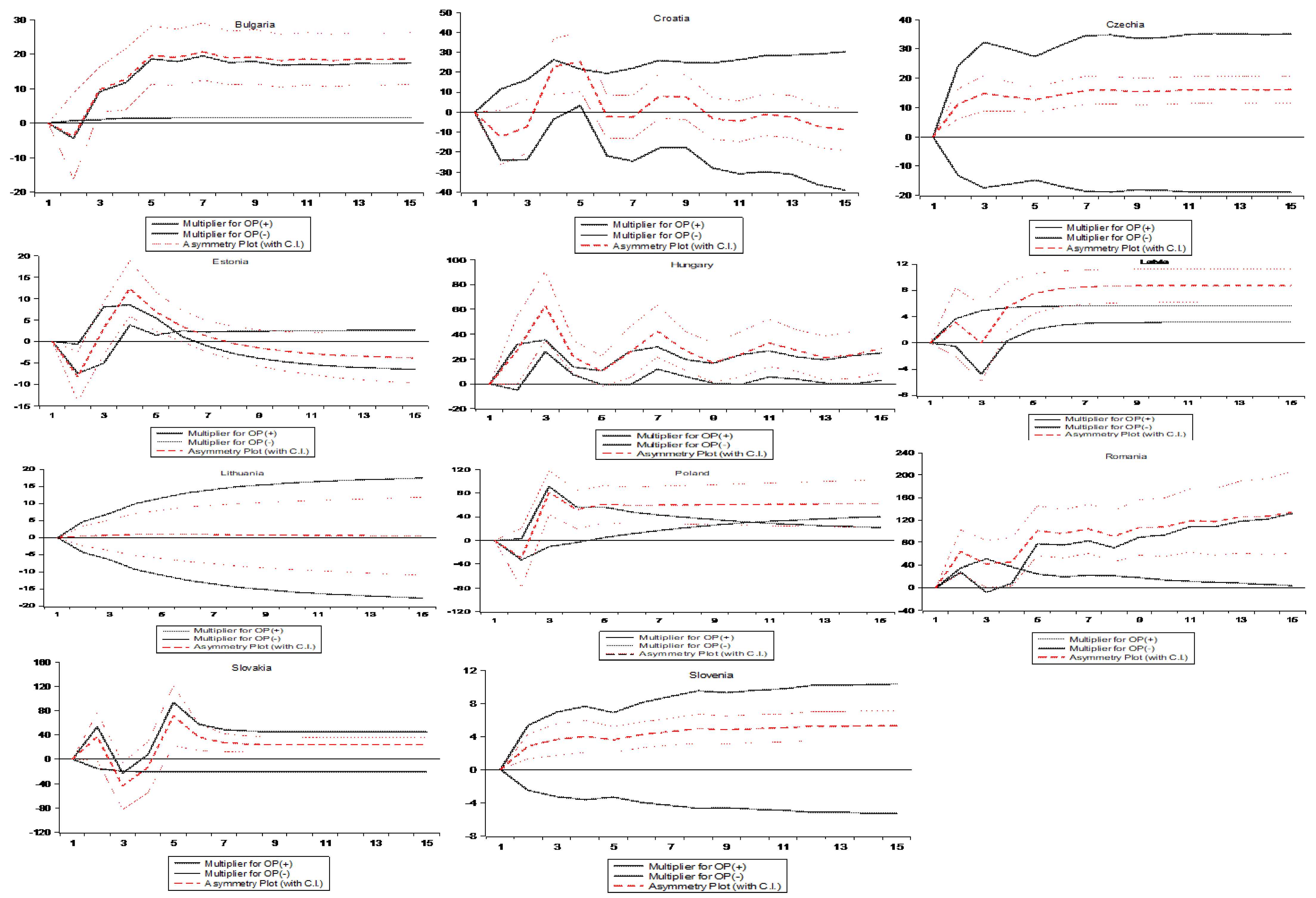
Figure 2.
Cumulative dynamic multiplier of natural gas price of the CESEE countries.
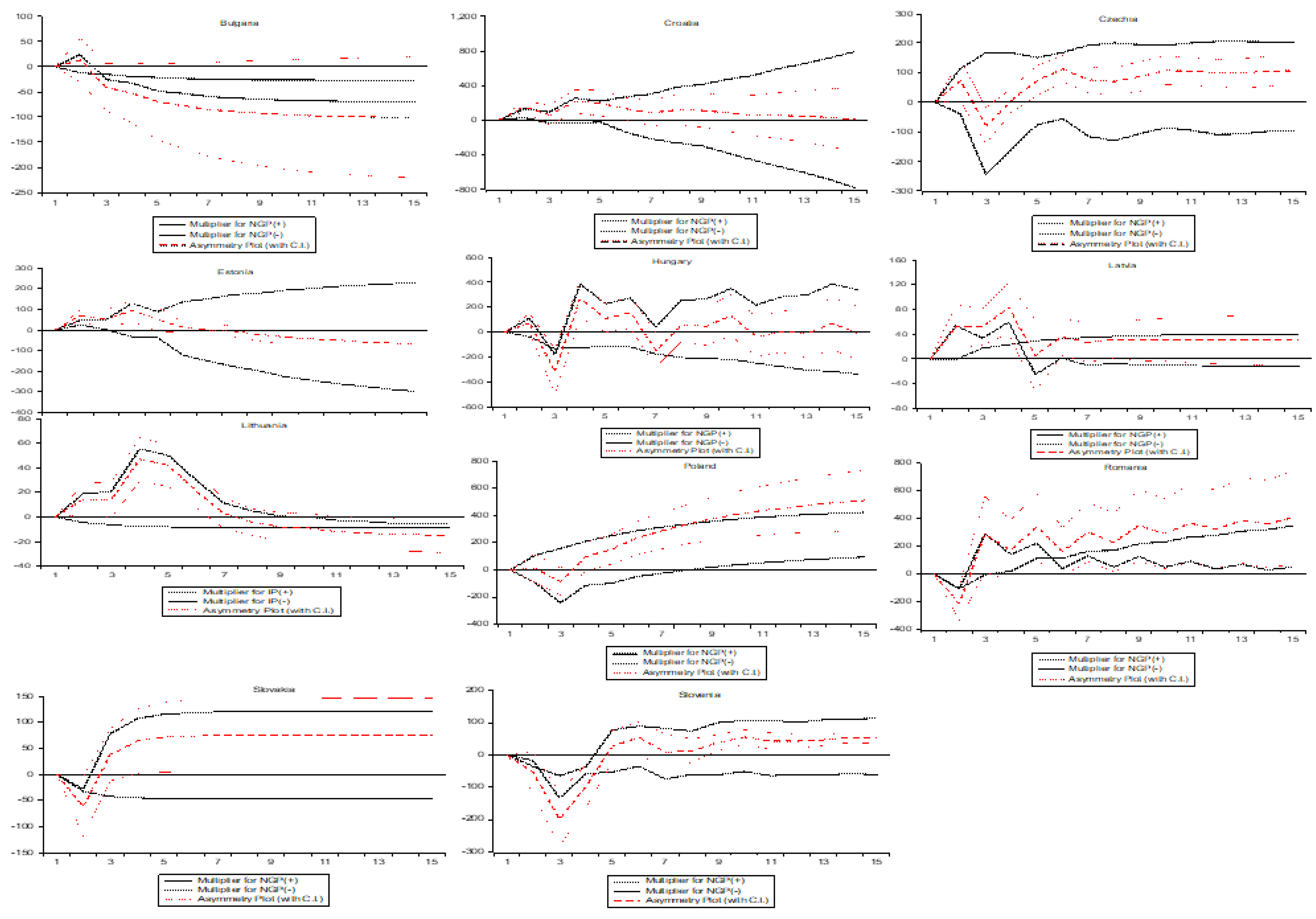
Figure 3.
Cumulative dynamic multiplier of industrial production of the CESEE countries.
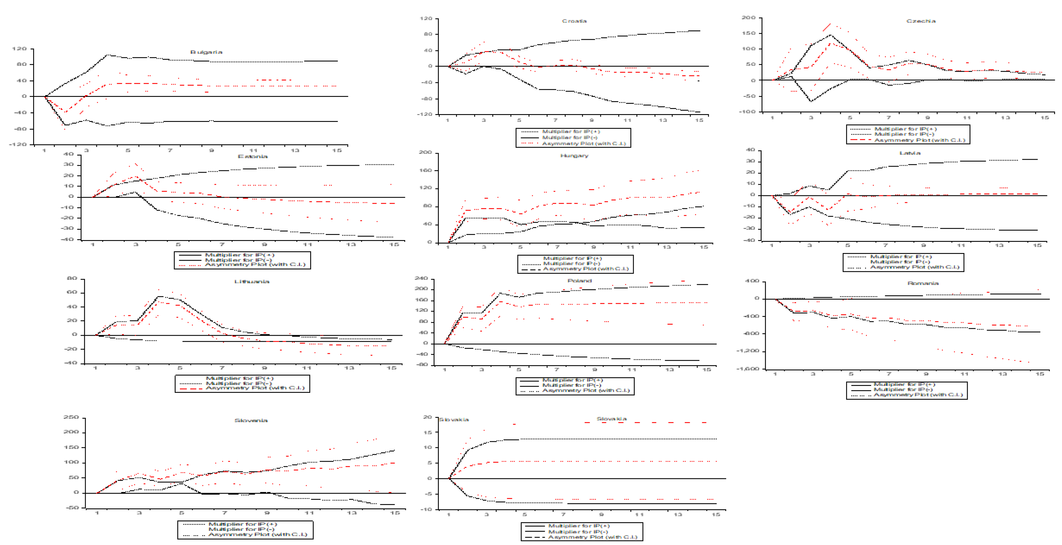
Figure 4.
Cumulative dynamic multiplier of wholesale prices of the CESEE countries.
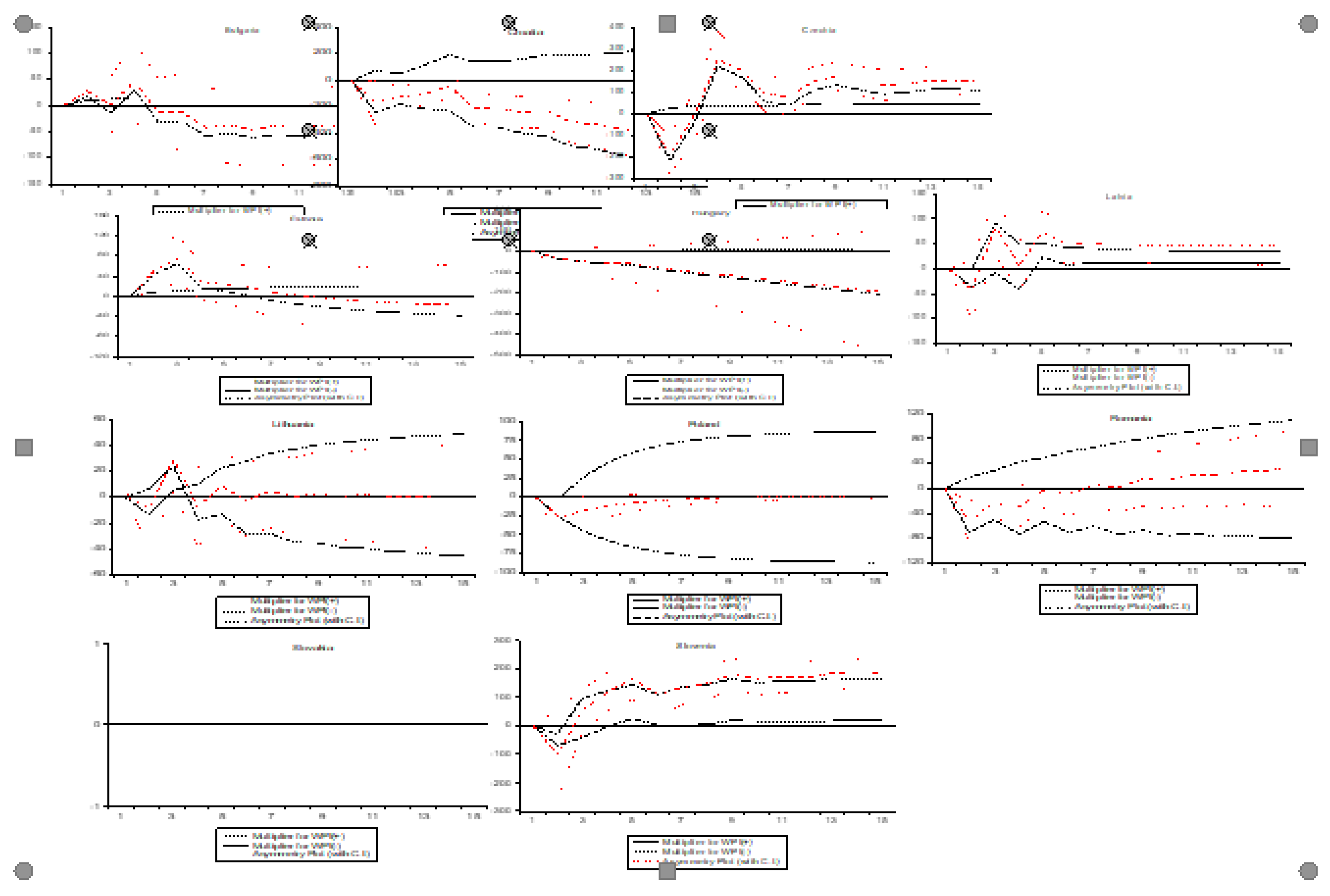
Figure 5.
Cumulative dynamic multiplier of exchange rate the CESEE countries.
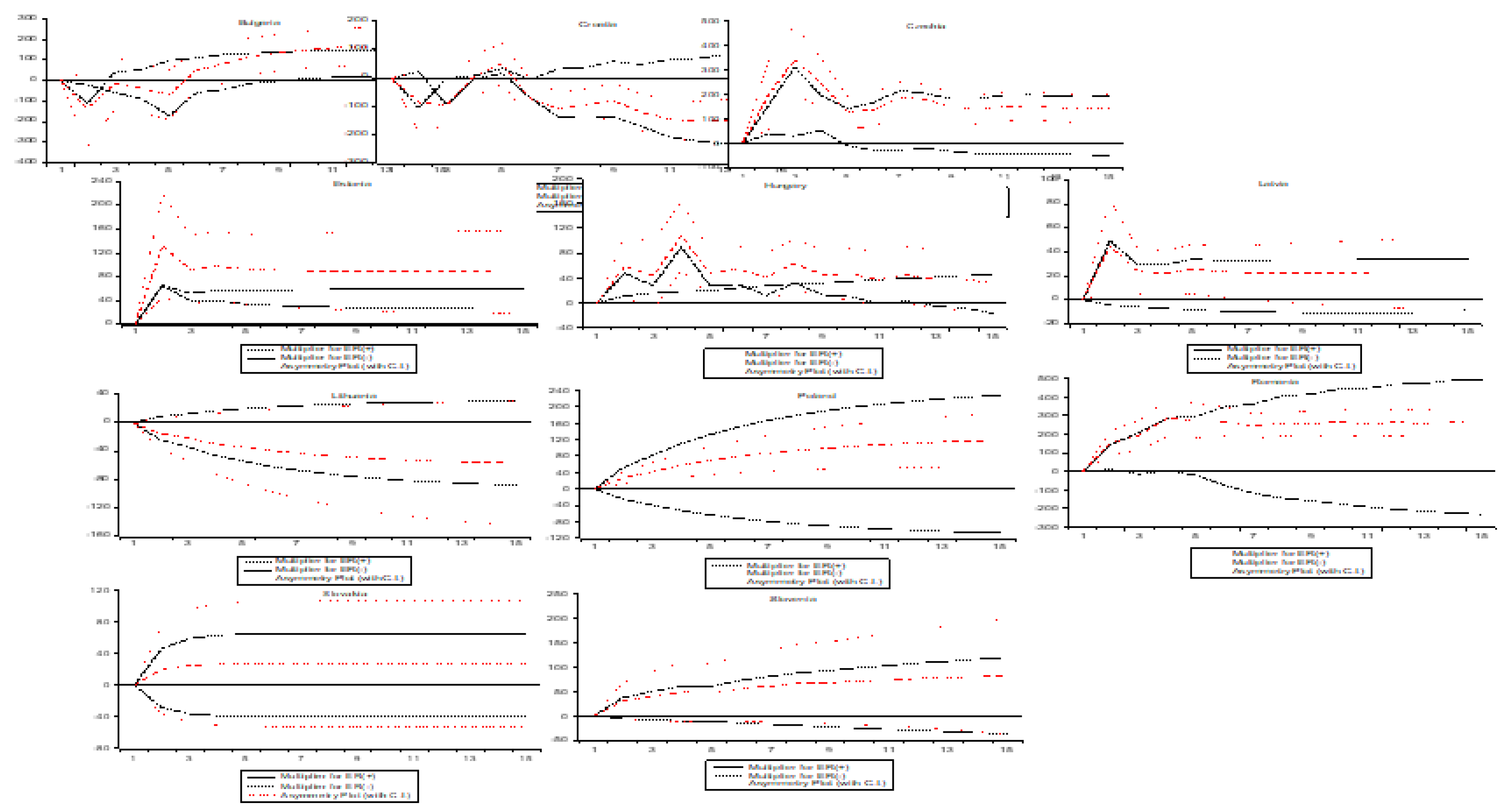
Table 1.
Review of the literature.
| Study | Methodology | Country | Findings |
| Bollino (2007) | Theoretical approach | US and China | |
| Varabei (2007) | VAR model, 1995Q1-2005Q1 | 10 net oil importing CEE countries | Mixed effect |
| Lutz and Meyer (2009) | Theoretical approach | Germany | Mixed effect |
| Kilian et al. (2009) | VAR model, 1975-2004 | 26 oil exporting and importing countries | Mixed effect |
| Rafiq et al. (2009) | VAR model,1993Q1-2006Q4 | Thailand | Negative effect |
| Korhonen and Ledyaeva (2010) | VAR model | 12 oil exporting and importing countries | Mixed effect |
| Bodenstein et al. (2012) | Global multicounty model, 2006Q1-2012Q1 | US | Positive effect |
| Tiwari et al. (2014) | Panel data model, 2005Q5- 2014Q1 | Gulf Cooperation Council (GCC) | Mixed effect |
| Allegret et al. (2015) | Panel smooth transition regression, 1980–2011 | 27 oil exporting countries | Positive effect |
| Chen et al. (2015) | Structural VAR, 1992-2012 | China and ASEAN countries | Positive effect |
| Bayar and Karamerikli (2015) | Hatemi-J cointegration test and Toda-Yamamoto causality test, 1997Q1-2015Q3 | Turkey | Negative effect |
| Huntington (2015) | Panel data model, 1984-2009 | 91 oil exporting and importing countries | Mixed effect |
| Rafiq et al. (2016) | Linear panel models, 1970-2010 | 28 oil exporting and importing countries | Mixed effect |
| Raheem (2017) | Non-linear ARDL, 1992Q1-2016Q6 | 6 oil exporting and importing countries | Mixed effect |
| Drachal (2018) | Granger causality test, 2000M1- 2015M12 | 5 CESEE countries | Mixed effect |
| Nasir et al. (2018) | TV-SVA model,1987Q2–2017Q2 | BRICS countries | Mixed effect |
| Taghizadeh-Hesary et al. (2019) | SEM model, 2000 Q1-2015Q4. | 21 oil exporting and importing countries | Mixed effect |
| Nasir et al. (2019) | SVARmodel,1980- 2016 | Gulf Cooperation Council (GCC) | Mixed effect |
| Baek and Kwon (2019) | NARDL model, 1992Q1-2017Q2 | Korea and ASEAN countries | Mixed effect |
| Ahad and Anwer (2020) | NARDL model, 1990Q1-2016Q4 | Pakistan | Negative effect |
| Alkhateeb and Mahmood (2020) | NARDL model, 1970-2018, 2001-2018, 1980-2018, 1994-2018 | Gulf Cooperation Council (GCC) countries | Mixed effect |
| Turan et al. (2020) | ARDL model, 1996Q1-2018Q1, 2004Q1-2017Q2, 1995Q1-2017Q2 | Czechia, Hungary and Poland | Mixed effect |
| Ahad and Anwer (2021) | NARDL model,1992Q1-2015Q4 | BRICS countries | Mixed effect |
| Abu Eleyan et al. (2022) | TVP-VAR model, 1990Q1- 2018Q4 | ASEAN countries | Mixed effect |
| Mirnezami et al. (2023) | GVAR model, 1980Q1-2020Q4 | 24 oil and gas exporting and importing countries | Mixed effect |
| Moshiri and Kheirandish (2024) | Panel VAR model,1980-2019 | 30 oil and gas exporting and importing countries | Mixed effect |
Source: Author’s compilation.
Table 2.
Estimation results of the asymmetric ARDL model.
| Variables. | Bulgaria | Croatia | Czechia | Estonia | Hungary | Latvia | Lithuania | Poland | Romania | Slovakia | Slovenia |
|---|---|---|---|---|---|---|---|---|---|---|---|
| Long run | |||||||||||
| -1.51*** | -0.37*** | -1.13*** | 0.06 | -0.23 | -0.68*** | -0.26 | -0.467*** | -0.200*** | -0.813*** | -0.507*** | |
| 42.43*** | 14.27 | 27.11*** | -24.14 | 32.96 | 7.79** | 40.93 | -36.53** | 90.38 | 73.99*** | -11.84** | |
| 18.63*** | -24.03*** | -40.63*** | -40.46 | -122.62 | -5.07*** | 32.87 | 9.76 | -133.89** | -1.81 | -16.91** | |
| 26.42*** | -393.77*** | -61.09 | 835.55 | 1095.20 | -30.59 | -536.33 | -8.71 | 219.27 | -104.40 | 181.01** | |
| 10.94 | -256.90*** | 16.78 | 745.94 | 1030.37 | -43.05** | -184.68 | -437.39*** | 1308.01** | 42.12 | 87.16 | |
| -17.71*** | 157.69*** | 0.46 | -427.94 | 90.59 | -16.56 | 75.49 | 1.42 | -362.04** | 127.22** | -0.40 | |
| -18.12*** | 666.78** | 512.87*** | -112.40 | -46.54 | -10.35 | -74.24 | -4.61** | -246.04** | 13.43 | 56.49 | |
| -0.21 | -123.81*** | 76.06*** | 163.14 | -76.18 | -20.92*** | -9.35 | -95.72*** | -96.24 | -91.64*** | -43.95** | |
| -19.46 | -65.08** | 80.26*** | -123.86 | 8.55 | -14.82** | 54.09 | -41.63 | 15.71 | -41.89 | 6.44 | |
| -18.32*** | 172.09 | -60.09*** | -351.46 | 38.79 | -7.41 | 8.86 | -85.32** | -284.21*** | -137.55*** | -2.83 | |
| -23.49 | 51.74 | -74.74** | -295.44 | 479.56 | -6.43 | -75.08 | -206.87*** | -468.21*** | 7.91 | -92.73 | |
| Short run | |||||||||||
| 14.93 | -16.11*** | 30.63*** | -6.40*** | 7.63 | -0.15 | -14.40** | -17.08 | 8.28 | 78.14*** | -6.01*** | |
| -25.74*** | -23.17*** | 25.63*** | -10.54*** | -16.91*** | -48.86*** | -57.86** | |||||
| -14.00** | -3.32 | -12.2** | -36.34** | -34.25 | |||||||
| -7.93** | -10.29 | 26.23 | 37.48 | ||||||||
| -5.27 | -9.01*** | 19.84** | 1.24 | 7.13 | -3.49*** | 8.56 | -6.63 | -26.79*** | -1.47 | 1.43 | |
| -40.53*** | -12.08*** | 25.10 | -10.64*** | -77.14*** | 8.65 | ||||||
| -25.29*** | 47.29*** | -6.58** | 10.42** | ||||||||
| 36.2*** | -4.15 | ||||||||||
| -106.22 | 8.96 | -89.35** | 12.43*** | -74.76** | 71.22*** | 31.26 | -204.54*** | -20.27 | 6.20 | -152.26 | |
| -428.43 | 77.00** | -119.14** | 53.96** | -423.70*** | 57.86*** | 137.50*** | 55.01 | -74.75*** | |||
| -485.73 | 81.19** | -368.43*** | 87.12*** | 102.63*** | -152.26** | ||||||
| -325.25 | 117.39** | -573.79*** | 135.64** | ||||||||
| 200.40*** | -96.33*** | 18.96 | -3.72 | 164.65** | -29.61*** | -82.64*** | -56.18 | -208.54 | 34.27 | -11.77 | |
| 71.39 | 102.34*** | 58.69*** | 134.11 | 15.47 | -224.8*** | -142.73 | 52.47 | ||||
| -109.92 | 25.39 | -240.28*** | -139.04*** | 50.14 | |||||||
| 59.88*** | |||||||||||
| 8.89 | 126.53*** | -387.39*** | 39.50*** | 20.98 | -39.52*** | 19.66 | 0.66 | -61.46*** | -17.44 | -54.77** | |
| 233.42*** | -38.79** | -117.52 | -28.23** | -22.45 | 68.63*** | -213.85** | -68.26** | ||||
| 180.38*** | 1.96 | 235.46*** | -17.76 | -45.45*** | 17.52 | ||||||
| 174.88*** | 126.25*** | 28.30 | 36.54** | ||||||||
| -246.71*** | 250.01*** | 339.45*** | -39.23** | 238.67 | -7.12 | -48.61** | -0.24 | -49.24*** | 10.93 | 28.68 | |
| 25.60 | 234.87*** | -314.89** | -16.35 | -30.90** | 1.32 | -51.23*** | |||||
| 131.74** | -387.75*** | -35.55** | 27.04 | 0.11 | -43.56*** | ||||||
| 1.73*** | |||||||||||
| -84.96*** | -15.76 | -5.16 | 3.93 | 27.25** | -14.39*** | -6.39 | 42.65 | -19.26 | 31.15 | -7.97 | |
| -25.94 | 55.36*** | 15.33** | 38.83** | 15.14*** | 141.51*** | 80.62*** | 26.06** | ||||
| 26.39** | -9.89 | 20.07 | 73.47** | 60.94** | 31.46*** | ||||||
| 9.98 | 34.55** | 58.73 | 51.44*** | ||||||||
| -2.77 | -7.15 | -0.33 | -8.02 | 5.30 | -0.88 | -5.80 | -76.92** | 112.32 | -34.08*** | -24.78** | |
| 3.19 | -14.74 | 0.84 | -33.80 | 10.69*** | -21.54** | -38.44*** | |||||
| -40.17** | -55.03** | -12.21 | -5.56 | 9.96*** | -33.18*** | -31.67*** | |||||
| -76.92*** | -18.19** | -39.85** | -24.33*** | ||||||||
| -20.08 | -64.33 | 67.90*** | 40.39 | 8.98 | -5.10 | 2.30 | 20.96 | -0.207 | -20.54 | -1.43 | |
| 13.08 | -87.47** | 44.21 | 138.32*** | 118.80 | |||||||
| -28.49 | 110.90** | 189.75 | |||||||||
| -124.28** | 91.36** | ||||||||||
| 137.85 | -115.10*** | -84.47** | -56.79 | 7.65 | -4.42 | -19.55 | -96.74*** | -75.02 | 6.44 | -47.08*** | |
| 55.99 | 37.30 | -98.68** | -41.03 | 28.09 | |||||||
| -16.85 | -87.22** | -34.59 | -128.70*** | 85.98*** | |||||||
| 172.78** | -113.13*** | -105.54*** | |||||||||
| ECM (-1) | -0.51*** | -0.37*** | -0.43*** | -0.06*** | -0.23*** | -0.68*** | -0.26*** | -0.46*** | -0.20*** | -0.81*** | -0.50*** |
| F-test | 9.56*** | 11.45*** | 7.43 | 8.43*** | 4.19*** | 9.00*** | 5.33 | 5.55*** | 7.05*** | 7.28*** | 8.58*** |
| t- test | -7.69*** | 3.81*** | -7.49 | -6.46*** | -7.21*** | -6.53*** | -8.33 | -5.51 | -9.36*** | -8.32*** | 3.61*** |
| Adju. R-sq. | 0.76 | 0.78 | 0.80 | 0.83 | 0.70 | 0.71 | 0.64 | 0.67 | 0.77 | 0.49 | 0.76 |
| Prob(F-statistics) | 0.000 | 0.000 | 0.000 | 0.000 | 0.000 | 0.000 | 0.000 | 0.000 | 0.000 | 0.000 | 0.000 |
| Wald Test | 36.85*** | 64.49*** | 80.10*** | 60.61*** | 61.441*** | 21.56*** | 8.04*** | 91.121*** | 173.38*** | 40.222*** | 60.237*** |
| CUSUM | Stable | Stable | Stable | Stable | Stable | Stable | Stable | Stable | Stable | Stable | Stable |
| CUSUMQ | Stable | Stable | Unstable | Stable | Unstable | Unstable | Stable | Stable | Stable | Stable | Unstable |
| LM | 0.456 | 0.326 | 0.143 | 0.383 | 0.172 | 0.171 | 0.512 | 0.689 | 0.879 | 0.128 | 0.941 |
| ND. | 0.890 | 0.254 | 0.265 | 0.237 | 0.699 | 0.499 | 0.689 | 0.364 | 0.991 | 0.457 | 0.870 |
| H | 0.504 | 0.729 | 0.181 | 0.626 | 0.824 | 0.934 | 7.903 | 0.915 | 1.528 | 1.254 | 1.850 |
| RESET | 2.263 | 1.132 | 3.294 | 5.145 | 3.630 | 4.658 | 1.687 | 1.987 | 9.075 | 4.155 | 10.256 |
Notes: TB – trade balance; OP- oil prices, NGP – natural gas price, WP- wholesale price, IP - industrial production, ER – exchange rate. F-test and t-test, Error-correction model ECM (-1), - Lagrange multiplier test (LM test), stability tests (Cusum and Cusumq), stable (S) and unstable (U), ND. - Normality test, H - Heteroscedasticity test, RESET – misspecification test. ***, ** and * indicate “statistical significance” at 1%, 5% and 10% levels, respectively. Source: Author’s compilation
Table 3.
Estimation results of the robustness check.
| Variable | Bulgaria | Croatia | Czechia | Estonia | Hungary | Latvia | Lithuania | Poland | Romania | Slovakia | Slovenia |
|---|---|---|---|---|---|---|---|---|---|---|---|
| Long run | |||||||||||
| -0.74*** | -0.27*** | -1.03*** | -0.39*** | -0.60*** | -0.70*** | -0.67*** | -0.56*** | -0.24*** | -0.81*** | -0.51** | |
| 47.17*** | -69.71*** | 20.89*** | 22.27** | -10.38 | 4.85 | 3.86 | -49.83 | 14.18 | 57.31*** | 17.76** | |
| -2.42 | -40.44** | 14.78** | 8.91 | 5.25 | -8.26*** | 1.67 | -30.32 | -99.44** | 17.80 | -5.16 | |
| 155.64 | 102.84 | -293.96*** | -35.28 | -75.88 | -87.47** | 15.71 | -797.07*** | -1034.8*** | -513.74 | -46.17 | |
| 104.42 | -310.91*** | -418.90*** | 30.39 | -445.22*** | 13.37 | 60.17 | -566.67 | -79.79 | -125.09 | 78.60 | |
| -143.84*** | -2.67 | -66.54*** | -61.45** | -20.86 | -11.30*** | 14.29 | 184.13 | -293.6*** | 102.12** | 71.85 | |
| 9.85 | 271.30 | 160.90*** | -73.63 | -15.86 | -34.03 | -37.28 | 181.30** | -52.32 | 9.98 | -8.59 | |
| -87.43*** | -195.02*** | 61.98** | -41.35 | -26.93** | -17.98*** | -28.14*** | 10.89** | 209.84** | -37.98 | -58.09** | |
| -94.30*** | -122.06*** | 70.20*** | -34.20** | 5.12 | -11.65** | -16.80 | 163.80** | 677.44 | 3.42 | 3.60 | |
| -126.81** | 339.71 | -64.78*** | 63.26** | 2.80 | 12.62 | 4.75 | -70.79 | -109.02 | 8.03 | 17.08 | |
| -158.47 | -58.27 | -216.26*** | -8.71 | -21.04 | -46.59*** | 35.82 | -242.86*** | -446.49*** | -119.16 | 5.56 | |
| Short run | |||||||||||
| 15.14 | -19.47*** | 27.67 | 0.09 | 12.96 | 3.39 | 2.62 | -70.49*** | -5.77 | 46.55** | -6.83 | |
| -13.18 | -5.02 | -45.41 | -27.16 | -10.27 | |||||||
| -41.30*** | 2.25 | -35.90 | -34.92** | -1.29 | |||||||
| -5.07 | -36.25 | -16.12*** | |||||||||
| -14.15** | -11.30*** | 15.33 | -0.87 | 16.82** | -5.78*** | 1.13 | -0.23 | -37.00* | 14.45 | 4.95 | |
| -10.87 | -10.9*** | -30.03*** | -41.79*** | -33.83* | |||||||
| 3.23 | -5.96** | 29.39*** | |||||||||
| 20.91*** | |||||||||||
| -87.09*** | 28.73 | 199.9 | -14.10 | -45.65 | 0.12 | 10.66 | 238.94 | 129.02 | -170.38 | -9.97 | |
| -171.42** | 362.4*** | 85.68*** | 582.36*** | 214.48 | 60.54 | ||||||
| -214.88** | -631.91*** | -105.13 | |||||||||
| -151.67 | |||||||||||
| 9.99 | -86.86*** | 434.5*** | -1.15 | -181.6** | -48.00 | -52.52 | -538.93*** | -547.39* | -691.61*** | 10.32 | |
| -164.9** | 29.8 | 155.3 | -41.54 | -191.69 | -105.18*** | ||||||
| -44.60 | |||||||||||
| 63.84*** | -0.74 | -339.83** | -5.84 | 57.48** | -7.96*** | -28.46*** | -0.99 | -16.68 | -8.09 | -40.35 | |
| 121.79*** | 20.43 | -6.84 | -252.87*** | 108.63** | -279.56*** | ||||||
| 108.71*** | 157.35*** | -41.43** | -134.39 | 40.00 | |||||||
| 116.32*** | 63.90* | ||||||||||
| -38.73 | 75.79 | 166.9*** | -22.2 | -9.54 | -23.82 | -27.41 | -147.96** | -51.51* | -238.09 | -4.39 | |
| -53.5 | -8.74 | -131.34 | 13.93 | ||||||||
| 38.32*** | 1.65 | 53.66** | |||||||||
| 3.29*** | |||||||||||
| -65.56*** | -38.38*** | 15.34 | 2.9 | -15.07 | -12.59*** | -2.06 | 67.22 | 69.21* | 48.30** | 8.11 | |
| 25.04*** | 62.34*** | 16.2*** | 48.4** | 14.14** | 106.53** | -16.29 | 62.76** | 49.80*** | |||
| 13.03*** | 42.48** | 3.71 | 150.88** | -26.53 | 40.37 | 31.95** | |||||
| 18.7** | 137.00** | -133.87** | 66.05*** | ||||||||
| -40.45** | -18.27 | -8.5 | 25.04** | -7.27 | -9.43 | -42.44 | 468.42* | 2.78 | -32.30 | ||
| 14.64 | 18.4** | -39.95** | -0.63 | -3.60 | -93.60*** | -18.57*** | |||||
| -31.39** | -10.95 | 1.97 | -22.22** | -96.21*** | |||||||
| -21.92 | -51.20*** | -10.5** | -27.57*** | -42.80 | |||||||
| 12.67 | -38.95 | 19.98 | 48.8 | 1.68 | 8.83** | -17.78 | 124.18** | 33.31 | -74.00 | 8.74 | |
| -20.15 | 92.00 | 57.1** | -31.17 | 115.10** | 22.09 | 168.04 | |||||
| -121.20** | 92.88** | -83.10*** | 68.07 | 91.48*** | |||||||
| -216.84*** | -45.55 | 88.0 | |||||||||
| 82.18 | -16.28 | -224.36*** | -12.07 | -32.62** | 24.30 | -136.51*** | -107.24*** | -96.78 | 2.84 | ||
| 127.90 | 46.66 | ||||||||||
| 178.43** | -95.72*** | ||||||||||
| 295.00*** | 95.93*** | ||||||||||
| ECM (-1) | -0.74*** | -0.27*** | -1.03*** | -0.39*** | -0.60*** | -0.70*** | -0.67*** | -0.57*** | -0.24*** | -0.81*** | -0.51*** |
| F-test | 9.077*** | 9.18*** | 8.34*** | 5.098*** | 6.88*** | 8.88*** | 4.13* | 6.94*** | 6.81*** | 7.82*** | 4.98*** |
| t- test | -6.39*** | 3.00** | -8.02*** | -3.10** | -7.52*** | -6.00*** | -5.71*** | -5.87*** | -394*** | -8.64*** | -2.49*** |
| Adju. R-sq. | 0.78 | 0.64 | 0.76 | 0.66 | 0.66 | 0.66 | 0.55 | 0.70 | 0.80 | 0.50 | 0.65 |
| Prob(F-statistics) | 0.000 | 0.000 | 0.000 | 0.000 | 0.000 | 0.000 | 0.000 | 0.000 | 0.000 | 0.000 | 0.000 |
| Wald Test | 5.83*** | 23.22*** | 5.60*** | 4.39*** | 10.43*** | 8.72*** | 3.65*** | 14.19*** | 32.14 | 6.59*** | 5.36 |
| CUSUM | Stable | Stable | Stable | Stable | Stable | Stable | Stable | Stable | Stable | Stable | Stable |
| CUSUMQ | Stable | Unstable | Unstable | Unstable | Unstable | Unstable | Unstable | Unstable | Stable | Unstable | Unstable |
| LM | 0.678 | 0.111 | 0.977 | 0.896 | 0.243 | 0.228 | 0.919 | 0.546 | 0.156 | 0.709 | 0.471 |
| ND. | 0.647 | 0.476 | 0.710 | 0.689 | 0.487 | 0.675 | 0.598 | 0.147 | 0.983 | 0.451 | 0.722 |
| H | 0.686 | 1.135 | 1.036 | 1.368 | 1.771 | 1.068 | 0.782 | 0.584 | 1.889 | 1.239 | 3.190 |
| RESET | 2.553 | 4.938 | 1.176 | 1.985 | 1.564 | 4.988 | 2.626 | 2.745 | 1.759 | 3.225 | 1.977 |
Notes: See Table 2. ***, ** and * indicate “statistical significance” at 1%, 5% and 10% levels, respectively. Source: Author’s compilation.
Disclaimer/Publisher’s Note: The statements, opinions and data contained in all publications are solely those of the individual author(s) and contributor(s) and not of MDPI and/or the editor(s). MDPI and/or the editor(s) disclaim responsibility for any injury to people or property resulting from any ideas, methods, instructions or products referred to in the content. |
© 2024 by the authors. Licensee MDPI, Basel, Switzerland. This article is an open access article distributed under the terms and conditions of the Creative Commons Attribution (CC BY) license (http://creativecommons.org/licenses/by/4.0/).
Copyright: This open access article is published under a Creative Commons CC BY 4.0 license, which permit the free download, distribution, and reuse, provided that the author and preprint are cited in any reuse.


