
Submitted:
02 October 2024
Posted:
03 October 2024
You are already at the latest version
Abstract
The present study examines the relationship between thermal and configurational entropy in two resistors in parallel and in series. The objective is to introduce entropy in electric circuits analysis by considering the impact of system geometry on energy conversion in the circuit. Thermal en-tropy is derived from thermodynamics, whereas configurational entropy is derived from network modelling. It is observed that the relationship between thermal entropy and configurational en-tropy varies depending on the configuration of the resistors. In parallel resistors, thermal entropy decreases with configurational entropy, while in series resistors, the opposite is true. The impli-cations of the maximum power transfer theorem and constructal law are discussed. The entropy generation for resistors at different temperatures was evaluated, and it was found that the con-sideration of resistor configurational entropy change was necessary for consistency. Furthermore, for the sake of generalization, a similar behavior was observed in time-dependent circuits, either for resistor-capacitor circuits or circuits involving degradation.
Keywords:
configurational entropy
; thermodynamic entropy
; constructal law
; electric circuit
; parallel and series equivalents
; maximum power transfer theorem
1. Introduction
Energy is inextricably linked to entropy, as its transformations are governed by the second law of thermodynamics. Although this statement applies to all forms of energy, the application of entropy is generally found in thermal energy conversion [1]. Its use in electrical circuit analysis is much less common [2] and a general agreement on its understanding has not been established yet. For instance, it is claimed that either entropy generation is maximal [3,4] or minimal [5,6]. Moreover, the state of the art on entropy in electrical circuits also describes the complexity of the circuit network configuration in terms of entropy, i.e., how the electrical elements are interrelated.
Considering that the theory of circuit analysis is well established, based on the conservation of charge and energy, and ultimately described by Kirchhoff’s circuit laws, we aim to evaluate if the use of entropy can clarify the intrinsic behavior of circuit analysis, for instance, in cases where the circuit can be at different temperatures, such as in the case of a battery. Thus, we will briefly describe the most valuable contributions of entropy from both a network point of view and thermodynamic point of view, in order to relate them in this contribution, and always keeping in mind that, as Jaynes explicitly stated, “We must warn at the outset that the major occupational disease of this field is a persistent failure to distinguish between the information entropy, which is a property of any probability distribution, and the experimental entropy of thermodynamics, which is instead a property of a thermodynamic state,[…] But in case the problem happens to be one of thermodynamics, there is a relationship between them” [7].
1.1. Network Entropy
Electrical networks have been investigated in terms of the drunkard’s walk problem, a well-studied situation in theory of probability [8,9,10,11] so that resistor networks can be interpreted in terms of probability. Nachmias developed a mathematical description of the physical network laws from voltage and current harmonic functions [11]. Perelson described thermodynamics in terms of networks and Kirchhoff laws [12], which is similar to the approach of this contribution, in which we apply thermodynamics to networks. Since a network is a connected graph endowed with positive edges such as resistances, there is an extensive literature on entropy in graphs theory [13,14]. Anand and Bianconi studied the entropy in networks [15], comparing Gibb’s, Shannon and Von Neumann entropies in networks describing microcanonical and canonical examples. Their results have been applied in several fields such as robotics [16], biophysics [17] or stock markets [18]. Finally, despite several references can be found for resistor networks, the presence of capacitors or inductors in the networks is much less common, being limited to the modelling of power lines [19], DC-DC converters [20] or with quantum effects [21], without playing an active role in the network entropy description.
1.2. Thermal Entropy in One Resistor
The entropy associated with energy conversion (thermodynamic entropy) is described by the relationship between current I (flow) and voltage V (gradient) in a resistor R described by Ohm’s law, V = I R. It is well established that when the current flows through the resistor, electrical energy is converted to heat and the thermodynamic entropy Stherm is generated in the resistor at a rate of
where TR is the resistor temperature [22] and Pdiss is the converted power into heat. In this basic configuration we have only one degree of freedom and Stherm describes how electrical energy is converted into thermal energy. It is worth noting that the entropy transferred to the environment at a temperature T is given by (1) plus the transferred entropy generation:
which is simply the Gouy-Stodola theorem [23]. In terms of entropy balance, the entropy change in the resistor , is due to entropy generation diS and exchanged entropy with the environment deS [22].
1.3. Literature Review of Thermal Entropy in Two Resistors
When two resistors are connected in parallel to a power source (Figure 1) a current divider is created.
The following derivation to find the electronic behaviour of the current divider from the minimisation of the entropy generation rate can be found in the literature [24,25]. The dissipated power Pdiss is given by:
where V is the voltage drop across the two resistors. The parallel configuration introduces the following constraint:
For linear relationship between fluxes and gradients (Ohm’s law):
And thus, the entropy generation rate is written as:
where T is assumed to be constant in an isothermal process with no temperature change at the resistors. For a steady state, it is claimed that if the entropy generation rate is minimized and equal to zero:
it leads to the expression of the current divider
Another approach to entropy in parallel resistor circuits is based on variational analysis. A review shows that maximum entropy production (MaxEP) and minimum entropy production principles (MinEP) can be applied [26] as long as the temperature is homogeneous [27]. Furthermore, Christen [25] pointed out the superiority of MaxEP as it is applicable far from the equilibrium while MinEP is restricted to near equilibrium, although no direct application to the electrical network is presented for MaxEP. Yet, a dynamic approach based on the theorem of minimum entropy production in linear systems with inertial effects showed that entropy can be split into excess entropy, related to dissipation and total entropy, including the inertial effects [28].
1.4. Degradation
Entropy is also present in systems undergoing degradation. Basaran pioneered its introduction in soldered joints [29,30] and developed the Unified Mechanics Theory as an attempt to combine mechanics and thermodynamics into a single discipline. Naderi et al. [31] applied to mechanical systems and, extending the application from mechanical systems to electrical systems our group has focused on electrical systems such as resistors, capacitors, LEDs or batteries along with energy degradation in terms of energy efficiency [32,33,34,35,36]. These studies only consider Sthem, and describe degradation to failure with an increase of Sthem up to a threshold [37].
1.5. Literature Gap and Paper Structure
When we reviewed the literature, some concerns were raised about the derivation (8-10) because the temperature is assumed to be the same in both resistors and therefore has no effect on the derivation. For the sake of illustration, we consider the counterexample where two resistors R1 and R2 are at different temperatures, T1 and T2. The entropy generation rate at R1 and R2 is respectively
Then, the total entropy generation rate is:
and minimising the entropy generation rate:
Hence
We note that the expression for the current divider is temperature dependent. Therefore, only in the case that T1= T2 we recover the expression obtained from Kirchhoff’s law. The discrepancy between (14) and Kirchhoff laws was tested experimentally with two variable resistors in order to have the same resistance at different temperatures (i.e., 1 kΩ at 25 ºC and 50 ºC), finding that the current profile obeys Kirchhoff’s current law (10) and minimum energy dissipation [38] but not the entropy minimisation described by (14).
Thus, it seems clear that a deeper analysis of the entropy of electrical circuits is worthy of further investigation for a number of reasons. Firstly, they are ubiquitous in modern technology. Secondly, constant temperature is a strong constraint that could have powerful applications in, for example, battery management where the role of entropy is ignored. Finally, the methodology can be straightforwardly generalised to other linear systems, as equivalent electrical circuits can be found in thermal management, biological applications [12] among others.
Within this framework, the objective of this manuscript is to evaluate the entropy of simple electronic circuits in order to elucidate the relevance of the network configuration expressed in terms of Sconfig and the energy conversion expressed in terms of Stherm.
The paper is organised as follows. First, we explain the methodology on how to calculate network entropies for circuits with resistors and capacitors, then we present the results entropy correlations for parallel and series configurations with voltage and current sources. We continue with two tree-shape networks and two sources circuits to clarify the influence of complexity in the thermal dissipation and finally we evaluate the impact of network configuration due to time dependent circuits in R-C configurations and degradation.
2. Materials and Methods
As mentioned in the introduction, we are concerned with two types of entropy, Sconfig related to network configuration and Stherm, related to energy conversion. Stherm is computed as described above in terms of voltage, current and temperature. Sconfig is calculated in terms of the probability of network configurations. We describe the analysis of the entropy calculation for two resistors in parallel, in the configuration shown in Figure 1. Applying Kirchhoff laws, we can write the relationship between currents and voltages in terms of a network matrix.
The probabilistic interpretation of this expression in terms of conductances can be found in [8], but for our purposes in relating it to thermal entropy we retain the resistive form. We aim to calculate the entropy of this matrix. As the matrix is diagonal, we can use the Shannon entropy using the expression:
This equation thus provides information about the configuration or complexity of the system, which in this case has two degrees of freedom. Landauer proposed this approach, but he did not develop it [38]. In this expression, p(x) represents the probability of current flowing through one resistor. Considering the two resistors together, and assuming a constant temperature T, the result is:
It can be seen that the probability of current flowing through one resistor or the other is simply given by the current divider solution given in (10). This gives us the configurational entropy of a circuit.
Another resistor configuration is two resistors in series (See Figure 2). In this case, the circuit considered is a voltage divider instead of a current divider, defined by:
We want to determine Sconfig using the same procedure that as for parallel resistors. The matrix is again diagonal:
Therefore,
In this particular case, Sconfig is the same for both parallel and series resistors. We extend this analysis to R-C networks, which are less common. Following our considerations on Sconfig, we notice that this circuit (Figure 3) has only one degree of freedom in the DC analysis and the entropy is zero.
If E is time-dependent, e.g., a sinusoidal source in steady state, then the capacitor impedance is frequency-dependent , which introduces a new degree of freedom. Accordingly, we can write Sconfig as
where ln (r eiθ) = ln r + iθ is the principal value of the logarithm. The use of complex Shannon entropy has already been studied [39,40].
To obtain Stherm for these circuits, we follow the description of the state of the art described in (12). For capacitive networks, Stherm can be evaluated either in the time domain or in the frequency domain, taking advantage of the invariance of energy and entropy under time transformations. For simplicity, we consider a single sinusoidal excitation signal characterised by its root mean square voltage (Vrms).
For completeness, we also investigate the time dependence in systems undergoing degradation. In this case, we consider Sconfig as a function of time, and Sthermal obtained from the time integration of the power. We consider three different types of degradation, described by a linear function,
a quadratic function
and an exponential function
which are commonly used in fatigue and breakdown studies. Each function describes material fatigue as an increase in Sconfig. In addition, we also introduce an entropy threshold with a Heaviside function, which describes structure breakdown, in case that it is reached. The multiplying constants in R2deg2 and R2deg3 are chosen to keep the degradation in the same range for t = 10 s. We substitute R2 for R2deg in entropy calculations.
3. Results
We present the results for resistor networks, evaluating the relationship of Sconfig and Stherm and relating both entropies. We conclude the analysis with two types of time-dependent circuits, R-C circuits and systems with degradation.
3.1. Entropy in Two Parallel Resistors
We evaluate Sconfig for different ratios of resistor pairs (Figure 4); the maximum entropy is found when the resistors are equal and decreases as their difference increases. Note that the graph is symmetrical with respect to the maximum found for R2/R1 = 1. Thus, from now on, without loss of generality, we will only plot curves for R2/R1 ≥ 1, as it is equivalent to having one resistor larger than the other.
Once Sconfig is characterised, we evaluate how energy is transferred through this system. The associated dissipation considering the E as a current source is given by
where Req = R1R2/(R1+R2). For a voltage source
For both sources, the generated thermodynamic entropy rate is
as in (1). If we assume a constant temperature T, as in electronic circuit analysis, for a fixed time, we obtain as illustrated in Figure 4. We use a normalised current source of 1 A, voltage source of 1 V and integration time of 1 s for calculations in all future calculations (in steady state ). We would like to point out that Stherm describes the conversion of electrical energy into thermal energy, whereas Sconfig describes the arrangement of the resistors. It is worth plotting the relationship between the two entropies for this circuit (illustrated in Figure 5). We consider Sconfig adimensional and Stherm with units JK-1; using a common unit would scale one axis.
The interest of this result lies in the fact that Stherm increases with Sconfig for voltage but decreases for current, i.e., the gradient (V) dissipates more energy as the complexity of the system increases, whereas the flow accommodates better as the complexity of the system increases. This result seems to be useful in other fields; for example, it might justify the constructal law [23,41]. We discuss this possibility in the discussions.
Having introduced the relationship between configurational and thermal entropy, we can consider the case of two resistors at different temperatures, which was the main motivation of the manuscript. The electrical properties of materials are temperature-dependent. We consider standard resistors whose resistance depends on temperature as:
where α is the temperature coefficient and for small temperature variations. The current divider becomes temperature-dependent at steady state:
The temperature coefficient can be either positive (for most of metals) or negative (for germanium and carbon for instance). In Figure 6, we plot the currents for the reference configuration (α = 0 and constant temperature), temperature-dependent resistors with α= 0.004 following (20), temperature-dependent resistors with α= -0.0005 and temperature-independent resistors (described by (14)). All examples are calculated with T1 = 300 K and T2 = 400 K. It can be seen that the curve for positive α is below the reference curve, as expected due to the increase in resistance with temperature whereas for negative α it is above. With regard to the case described by (14), we note that it is above the reference case, which is impossible, meaning that it is not possible to change the temperature of the material without changing its configurational properties. Therefore, in order to minimise the entropy generation, we have to consider the change in Sconfig due to thermal variation. This is a kind of Maxwell’s demon [42], where α = 0 means that we have a system (the resistors) that allows energy to be converted from electricity to heat without modifying the circuit, i.e., without assuming any change in the entropy of the system and violating the second law of thermodynamics.
As the resistance changes due to the temperature difference, Sconfig is modified accordingly:
the difference between the two cases is depicted in Figure 7. The overall magnitude does not change because we are plotting the normalised R2/R1, but the peak is shifted as:
Similar behaviour is found for Stherm (Figure 8), where we considered either a normalised current source of 1 A or a normalised voltage source of 1 V to estimate Stherm.
Finally, we evaluate Stherm with respect to Sconfig for the reference case and the temperature-dependent case (see Figure 9). The difference between the curves is related to the entropy of the resistor, both configurational, due to the resistor structural changes associated with resistance variation, and thermal, due to the different heat dissipations. We also point out that this behaviour is the same for both positive and negative α. and symmetrical for a voltage source as in Figure 5.
3.2. Entropy in Series Resistors
We carry out the same procedures as for a parallel configuration in a series configuration (see circuit in Figure 2). To find for a voltage source, we can write
And for a current source
The relationship between Sconfig and Stherm for series resistors is illustrated in Figure 10, as we have done for parallel resistors in Figure 5. For a voltage source, we observe an increase of thermal dissipation with complexity. The point of maximum Sconfig corresponds to R1 = R2. It is worth noting the relationship with the principle of maximum power transfer in a voltage divider, which occurs for R1 = R2. Maximum power transfer occurs when both entropies are at their maximum, i.e., when the complexity of the system is at its maximum and also the heat dissipation is at its maximum.
Now consider the maximum power in the case of a current source. We can transform the circuit in Figure 9 using the Norton equivalent to obtain a current source of magnitude I=V/R1. In this case,
which shows the validity of the maximum power transfer theorem for current sources. Note that (34) and (25) are different and only equal in the case where R1 = R2, the limit case. Note also that this case is different from the case depicted in Figure 5, where the current is I and here it is V/R1.
3.3. Tree Shape Networks
Previous results in Figure 5 suggested the possibility of constructual law justification. To further investigate this possibility, we analyse typical structures proposed in the constructal law literature such as river basins and capillary’s networks [23]. We considered two tree-shaped networks, with three and seven elements respectively and we computed Sconfig and Sthermal. The network structure and entropy results are given in
Figure 12 for three elements and in Figure 13 for seven elements. We considered a voltage source of 1 V and compared R3 with 1 Ω and 10 Ω in both cases. The arrows shown in
Figure 12d point to the maximum Sconfig. The physical interpretation is given in the discussions section.
3.4. Circuits with More Than One Source
Once we have evaluated circuits with a different number of resistors, we study now circuits with more than one power source. We add a voltage source V2 in series to R1 with E as the voltage source (See Figure 14a). We calculate the power dissipated in R1 and R2 by V1 and add the dissipated power by V2. The relevant question here is to analyse Sconfig. Note that if we remove the voltage sources (as it is usually done to calculate the Thévenin equivalent resistance), we have exactly the same circuit of two resistors in parallel. That is, despite the introduction of an additional power source, the configuration of the circuit does not change. Sconfig is therefore the same as for resistors in parallel. In Figure 14b we plot the Sconfig - Sthermal relationships for V2 = 0 (same case as in section 3.1), for V2 = 1 V and in series with R1, and for V2 = 1 V in series with R2 integrated for 1 s. The general shape of the curves is the same, and their differences are due to the different power dissipation in the three cases.
3.5. Time Dependent Entropy in a R-C System
We describe the results for a resistor in series with a capacitor (see the circuit in Figure 3). Following the same methodology described for resistors we evaluate the configurational and thermal entropies. Thus, we briefly describe the behaviour of the entropy in terms of the degrees of freedom of the circuit, R, C and ω, illustrated in Figure 15 as a function of frequency and Nyquist plot (Figure 16). We can see that the maximum configurational entropy is found at typical cut-off frequency and is equal to 1.132. Also, in the Nyquist plot, we find that the maximum entropy corresponds to the only real point in the plot. Both results are obtained from (21). Also, in the limit of low and high frequencies, Sconfig tends to 0, which is reasonable since the capacitor is either short-circuited or open circuit and thus, we have only one degree of freedom and entropy nulls. It should be remembered that at the cut-off frequency, the impedance modulus of the resistor and the capacitor are equal, which is consistent with the previous results of finding the maximum power transfer at the maximum configurational entropy.
Having presented the configurational entropy, we analyse the relationship between circuit configuration and energy conversion (Figure 17). First, we consider E a constant voltage source. The energy stored in the capacitor when fully charged is Integrating over the entire capacitor charge, the energy lost at the resistor during the charging process is , which is independent of R and the frequency, and thus, Sconfig is null.
Secondly, we consider E as a sinusoidal source. In this case, the power dissipated at the resistor depends on the root mean square voltage Vrms, where E is the amplitude of the sinusoidal.
And the generated entropy is:
The relationship between Sconfig and Stherm (integration of over time), depicted in Figure 17, illustrates a similar behaviour to that found for resistors, justifying the feasibility of applying the method to linear systems in general.
3.6. Time-Dependent Entropy for Degradation
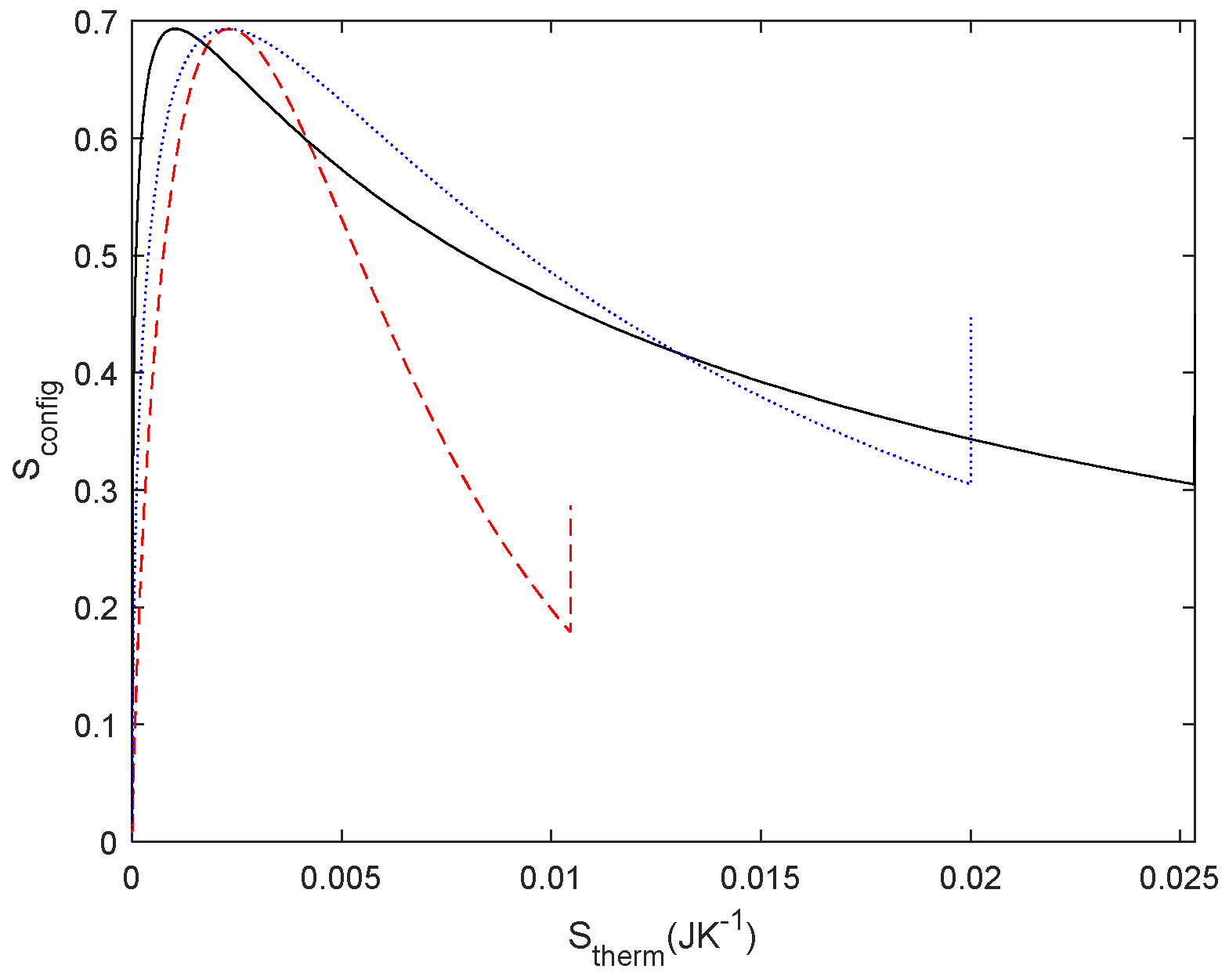
Following the degradation functions proposed in the Section 2, we study the effect of the degradation of a resistor in a parallel resistor network (Figure 18a) as a function of time in order to obtain Sconfig (t) (Figure 18b), Stherm (t) (Figure 18c) and their relationship (Figure 18d). The abrupt change in behaviour at t = 10 s is due to the Heaviside function. The different degradation mechanisms lead to different Sconfig – Stherm relationships, showing that the method is valuable for investigating systems that evolve with time. Moreover, it may be significant that the entropy generation rate thermal is independent of the degradation mechanism, as long as only Sconfig and thermal are involved in the degradation process due to R2, but it deserves further investigation.
thermal.
4. Discussion
So far, we have obtained valuable results that are worth discussing: the entropies relation, the effect on constructal law and the theorem of maximum power transfer, and the effect of time on entropy in R-C circuits and degradation.
We can begin with entropy itself. It is found in literature a discussion between Claude Shannon and John Von Neumann about entropy. C. Shannon said “My greatest concern was what to call it. I thought of calling it ‘information,’ but the word was overly used, so I decided to call it ‘uncertainty.’ When I discussed it with John von Neumann, he had a better idea. Von Neumann told me, ‘You should call it entropy, for two reasons. In the first place your uncertainty function has been used in statistical mechanics under that name, so it already has a name. In the second place, and more important, no one really knows what entropy really is, so in a debate you will always have the advantage.
”. Whether the story is true or not, it is certain that the concept of entropy still generates some debates on its interpretation and, as a physical magnitude and a mathematical property, it is worth devoting more research effort to it.
We use the quote to point out that they were probably both right. Entropy is a mathematical property that can be applied in different disciplines, but it has a different physical meaning in each problem. As mentioned above, Jaynes prevents us from confusing information entropy and thermodynamic entropy unless we are dealing with thermodynamic problems. So what we have tried to investigate in this paper is not whether they are the same thing, but how they are related, as there are two types of entropies describing different characteristics of the system: this is the purpose of relating Sconfig to Stherm. Stherm is clearly related to energy conversion, i.e., when the energy enters the circuit it is converted into heat. Sconfig is related to network structure, and is either decided by us, i.e., we decide whether to design a series or parallel circuit, or it evolve naturally over time due to degradation induced by energy dissipation. It is important to note that if the relationship R2/R1 ratio changes due to energy dissipation, we have a causal relationship between Sconfig and Stherm. Conversely, if we change the ratio arbitrarily or manually, there is a correlation, but not a causal relationship between Sconfig and Stherm. The same happens with temperature, and here we find the origin of the problem inferred from (14). We found that the change in entropy of the resistor (system) was not previously considered when its temperature changed. Taking this into account, the relationship Sconfig – Stherm helps to clarify the understanding that we can consider the entropy as a function of state of Sconfig and Stherm for the network system, but we also need to consider the entropy change in the universe to introduce the change in the network.
In order to investigate both entropies, as to our knowledge, entropies of a system are not usually correlated in complex systems, we investigate how energy is transformed in a linear system as a function of the network configuration. On the one hand, Sconfig was derived from a probability of the electrical circuit, and on the other hand, Stherm is inferred from thermodynamic relations. Understanding entropy derived from a probability allows us to deal with causal and not-causal systems. Obviously, Stherm is causal because it is governed by the laws of thermodynamics. But Sconfig is not causal, the network change is decided by the design of the electric circuit. In probability, if the system is not causal, the probability spaces are likely to be independent in many cases, and thus, the probabilities can be computed as independent. In our opinion, this approach allows an interdisciplinary approach to complex problems, as it allows to deal with different properties of the system to be treated with the same magnitude. For instance, the studied Sconfig and Sthermal are independent as long as Sconfig is not modified by the same energy. This explanation is consistent with the constructal law, as we proposed in the results section, which states that “for a finite size flow to persist in time (to survive) it must evolve in such a way that it provides easier and easier access to the currents that flow through it” [23] and to our knowledge, it has not been illustrated using this approach, which can help to clarify its understanding. For a better understanding of it, we considered the typical examples of this law, such as tree-shaped structures, that can be found either in rivers or blood capillaries. To gain a deeper insight into this result, we obtained the entropies correlation for a tree-shaped structures with three and seven elements (See
Figure 12 for three elements and in Figure 13 for seven elements). In these networks, the symmetry of the resistor configuration is broken and thus, Sconfig (R2/R1) is not symmetric anymore. It is important to note that the maximum of Sconfig corresponds to an extreme of the Stherm. As indicated by Bejan, the design of the structure organizes to fit the flows. From our results, and in other words, the organisation obeys a causal relationship between the energy involved in the process and the final network structure. From Bejan’s definition, we had understood that design configured the energy Sconfig – Stherm but it seems to be more convenient to plot Stherm – Sconfig. For instance, replotting Figure 18 (d) with the axis exchanged, it is easy to write a function Sconfig = f(Stherm) as illustrated in Figure 19 so that constructal law satisfies the condition
And the correlation between both entropies leads to a maximum in which the constructal law is satisfied. This approach therefore opens up the possibility of exploring a law for the dual (gradients), which has not been considered before, since gradients behave similarly to flows and also of exploring causal and non-causal interdisciplinary problems.
Continuing with the constructal law applied to resistors, we can also interpret that (17) depends on the geometry if we consider that the resistance is given by R=ρ l/A, where ρ is the resistivity, l is the length and A is the area of the resistor. This agrees with the relationship between geometry design and energy dissipation given in the law.
Another interesting result concerns the theorem of maximum power transfer. This theorem is traditionally derived from a minimisation process of the energy transferred. In Figure 10, we found that the minimum point corresponds to the theorem. It is not surprising that this theorem depends simultaneously on the network and thermal entropies, since its classical derivation minimises the power for the network. However, using our approach Sconfig = f(Stherm), we can have a better understanding of the power transfer not only at the extremal point but also as a function of the network configuration, allowing further predictions of circuit performance.
Regarding the increase in complexity with more resistors or power sources, we can point out that changing the power sources affects the energy conversion but not the network configuration, and thus, while Stherm changes, Sconfig remains the same. On the contrary, increasing the number of resistors in the network introduces an entropy term for each resistor, thus changing Scon This is an interesting issue that we can discuss using the 3-resistors circuit illustrated in
Figure 12a. From an electrical point of view, we can connect the resistors in parallel and in series to find the equivalent resistor. The dissipated power will be the same for R1, R2 and R3, R1+R2//R3 or Req = (R1+R2//R3) where // means connected in parallel. However, the entropies associated with each case, assuming all resistors with R = 1 Ω, are 0.9634, 0.6365 and 0 respectively. Obviously, the entropy decreases as the circuit simplifies.
Time-dependent results are also interesting. On the one hand the degradation studies and on the other hand, the complex entropy in R-C systems. Degradation is a causal constraint of network modification due to energy dissipation, which can be described by Sthermal. We proposed three arbitrary time-dependent curves. We previously investigated the physical degradation of resistors [32] and capacitors [33], having established the interest of . In this contribution, we have confirmed the interest not only of this entropy but also of Sconfig, which had already been pointed out in [32] as a possible explanation of the fatigue and breakdown of the resistor. An interesting result, which could be worthy of further research, is that the relationship between Sconfig and is invariant to the degradation mechanism, as long as they are the only entropies involved in the process. However, Sconfig and Sthermal are dependent on the degradation mechanism. Both results can be useful for degradation characterisation, in order to complement the approaches given in [32,37].
The presence of imaginary entropy in R-C configuration is related to the time-dependent behaviour of the capacitance. However, it is striking that when the real part is maximum, and the imaginary part is zero, the entropy is maximum, which also corresponds to the same impedance modulus of the resistance and the capacitance at the point of maximum power transfer ratio. This behaviour could be further investigated in terms of active and reactive power.
5. Conclusions
In conclusion, the thermodynamic analysis of a simple electric circuit has yielded valuable conclusions, as we have clarified relationships between entropies. Firstly, we have related two different entropies that describe two different characteristics of the system. In particular, the relationship between configurational entropy and thermal entropy in different linear electric circuits provides a clear illustration of how energy transformation is related to the structure of the system on which it is transformed. Secondly, the relationship between current flow and geometric design is highlighted as an explanation for the constructal law, which describes how a system must change to accommodate an entropy change. Thirdly, the change in configurational entropy due to a temperature difference is demonstrated to justify the thermal dissipation of the electric circuit. Fourthly, it is shown that the maximum power transfer theorem satisfies an entropy maximum, both for thermal and configurational entropies. Finally, the methodology was extended to R-C systems, resulting in a dependence similar to that observed in resistors. It is anticipated that these results, derived from simple examples, can be generalized to more complex systems.
Author Contributions
Conceptualization, AC.; methodology, AC; software, AC; validation, AC; formal analysis, AC and VJO; investigation, AC; data curation, AC.; writing—original draft preparation, AC.; writing—review and editing, VJO and HM.; funding acquisition, HM. All authors have read and agreed to the published version of the manuscript.
Funding
This research was funded by the Spanish Ministerio de Ciencia, Innovación y Universidades (MICINN)-Agencia Estatal de Investigación (AEI) by project PID2022-138631OB-I00. Grant and PID2022-139479OB-C21 funded by MICIU/AEI/ 10.13039/501100011033 and by “ERDF/EU”.
Data Availability Statement
Dataset available on request from the authors
Conflicts of Interest
The authors declare no conflicts of interest. The funders had no role in the design of the study; in the collection, analyses, or interpretation of data; in the writing of the manuscript; or in the decision to publish the results.
References
- Bejan, A. Thermodynamics today. Energy 2018, 160, 1208–1219. [Google Scholar] [CrossRef]
- Harsha, N.R.S.; Prakash, A.; Kothari, D.P. The foundations of electric circuit theory; 2016; ISBN 9780750312660.
- Županović, P.; Juretić, D.; Botrić, S. Kirchhoff’s loop law and the maximum entropy production principle. Phys. Rev. E - Stat. Nonlinear, Soft Matter Phys. 2004. [Google Scholar] [CrossRef]
- Martyushev, L.M.; Seleznev, V.D. Maximum entropy production principle in physics, chemistry and biology. Phys. Rep. 2006, 426, 1–45. [Google Scholar] [CrossRef]
- Feynman, R.P.; Leighton, R.B.; Sands, M.L. The Feynman lectures on physics; Basic Books,: New York:, 2010; ISBN 9780465023820. [Google Scholar]
- Miranda, E.N.; Nikolskaia, S. Producción de entropía en circuitos eléctricos sencillos entropy production by simple electrical circuits. 2004.
- Jaynes, E.T. (Edwin T.. Probability theory: the logic of science; Bretthorst, G.L., Ed.; Cambridge University Press: Cambridge, 2003; ISBN 0521592712. [Google Scholar]
- Doyle, P.G.; Snell, J.L. Random Walks and Electric Networks. By Peter G. Doyle and J. Laurie Snell; The Mathematical Association of America, Inc. 1984. [Google Scholar]
- Roy, R. Ohm’s Law, Kirchoff’s Law and the Drunkard’s Walk 2. The Drunkard’s Walk. Resonance 1997, 2, 33–38. [Google Scholar] [CrossRef]
- Roy, R. Ohm’s law, Kirchoff ’s law and the Drunkard’s walk: 1. Related electrical networks. Resonance 1997, 2, 36–47. [Google Scholar] [CrossRef]
- Nachmias, A. Random Walks and Electric Networks. In Lecture Notes in Mathematics; 2020; Vol. 2243, pp. 11–31.
- Perelson, A.S. Network thermodynamics. An overview. Biophys. J. 1975, 15, 667–685. [Google Scholar] [CrossRef]
- Li, X.; Wei, M. Graph Entropy: Recent Results and Perspectives. Math. Found. Appl. Graph Entropy 2016, 133–182. [Google Scholar]
- Dehmer, M.; Mowshowitz, A. A history of graph entropy measures. Inf. Sci. (Ny). 2011, 181, 57–78. [Google Scholar] [CrossRef]
- Anand, K.; Bianconi, G. Entropy measures for networks: Toward an information theory of complex topologies. Phys. Rev. E - Stat. Nonlinear, Soft Matter Phys. 2009, 80. [Google Scholar] [CrossRef]
- Caravelli, F. Trajectories entropy in dynamical graphs with memory. Front. Robot. AI 2016, 3, 179782. [Google Scholar] [CrossRef]
- Liu, C.; Ma, Y.; Zhao, J.; Nussinov, R.; Zhang, Y.C.; Cheng, F.; Zhang, Z.K. Computational network biology: Data, models, and applications. Phys. Rep. 2020, 846, 1–66. [Google Scholar] [CrossRef]
- Zhu, J.; Wei, D. Analysis of stock market based on visibility graph and structure entropy. Phys. A Stat. Mech. its Appl. 2021, 576, 126036. [Google Scholar] [CrossRef]
- Gupta, S.; Yadav, V.K.; Singh, M. Optimal Allocation of Capacitors in Radial Distribution Networks Using Shannon’s Entropy. IEEE Trans. Power Deliv. 2022, 37, 2245–2255. [Google Scholar] [CrossRef]
- Cheng, L.; Bi, C.; Kang, Q.; He, J.; Ma, X.; Zhao, L. Study on Entropy Characteristics of Buck-Boost Converter with Switched Capacitor Network. 2021 IEEE IAS Ind. Commer. Power Syst. Asia, I CPS Asia 2021. [CrossRef]
- Freitas, N.; Delvenne, J.C.; Esposito, M. Stochastic and Quantum Thermodynamics of Driven RLC Networks. Phys. Rev. X 2020, 10, 31005. [Google Scholar] [CrossRef]
- Lebon, G.; Jou, D.; Casas-Vázquez, J. Understanding non-equilibrium thermodynamics: Foundations, applications, frontiers; Springer-Verlag: Germany, 2008; ISBN 9783540742517. [Google Scholar]
- Bejan, A. Advanced Engineering Thermodynamics; Wiley: New Jersey, USA, 2006. [Google Scholar]
- Herrmann, F. Simple examples of the theorem of minimum entropy production. Eur. J. Phys. 1986, 7, 130–131. [Google Scholar] [CrossRef]
- Christen, T. Application of the maximum entropy production principle to electrical systems. J. Phys. D. Appl. Phys. 2006, 39, 4497–4503. [Google Scholar] [CrossRef]
- Sree Harsha, N.R. A review of the variational methods for solving DC circuits. Eur. J. Phys. 2019, 40. [Google Scholar] [CrossRef]
- Bruers, S.; Maes, C.; Netočný, K. On the validity of entropy production principles for linear electrical circuits. J. Stat. Phys. 2007, 129, 725–740. [Google Scholar] [CrossRef]
- Rebhan, E. Generalizations of the theorem of minimum entropy production to linear systems involving inertia. Phys. Rev. A 1985, 32, 581–589. [Google Scholar] [CrossRef]
- Basaran, C.; Yan, C. Damage Mechanics of Solder Joints. J. Electron. Packag. 1998, 120, 379–384. [Google Scholar] [CrossRef]
- Basaran, C.; Nie, S. A thermodynamics based damage mechanics model for particulate composites. Int. J. Solids Struct. 2007, 44, 1099–1114. [Google Scholar] [CrossRef]
- Naderi, M.; Amiri, M.; Khonsari, M.M. On the thermodynamic entropy of fatigue fracture. Proc. R. Soc. A Math. Phys. Eng. Sci. 2010, 466, 423–438. [Google Scholar] [CrossRef]
- Cuadras, A.; Crisóstomo, J.; Ovejas, V.J.V.J.; Quilez, M. Irreversible entropy model for damage diagnosis in resistors. J. Appl. Phys. 2015, 118, 2016. [Google Scholar] [CrossRef]
- Cuadras, A.; Romero, R.; Ovejas, V.J.V.J. Entropy characterisation of overstressed capacitors for lifetime prediction. J. Power Sources 2016, 336, 272–278. [Google Scholar] [CrossRef]
- Cuadras, A.; Yao, J.; Quilez, M. Determination of LEDs degradation with entropy generation rate. J. Appl. Phys. 2017, 122. [Google Scholar] [CrossRef]
- Rico, A.; Ovejas, V.J.; Cuadras, A. Analysis of energy and entropy balance in a residential building. J. Clean. Prod. 2021, 333, 130145. [Google Scholar] [CrossRef]
- Cuadras, A.; Miró, P.; Ovejas, V.J.; Estrany, F. Entropy generation model to estimate battery ageing. J. Energy Storage 2020, 32, 101740. [Google Scholar] [CrossRef]
- Basaran, C. Introduction to Unified Mechanics Theory with Applications; Springer Nature Switzerland, 2021. 2021.
- Landauer, R. Stability and entropy production in electrical circuits. J. Stat. Phys. 1975, 13, 1–16. [Google Scholar] [CrossRef]
- Nalewajski, R.F. Complex entropy and resultant information measures. J. Math. Chem. 2016, 54, 1777–1782. [Google Scholar] [CrossRef]
- Qian, G.; Iu, H.H.C.; Wang, S. Complex Shannon Entropy Based Learning Algorithm and Its Applications. IEEE Trans. Veh. Technol. 2021, 70, 9673–9684. [Google Scholar] [CrossRef]
- Reis, A.H. Constructal theory: From engineering to physics, and how flow systems develop shape and structure. Appl. Mech. Rev. 2006, 59, 269–282. [Google Scholar] [CrossRef]
- Zemansky, M.W.; Dittman, R.H. Heat and Thermodynamics; McGraw-Hill: USA, 1990. [Google Scholar]
Figure 1.
Current divider with two resistors in parallel. E describes a power source, either of voltage or current.
Figure 1.
Current divider with two resistors in parallel. E describes a power source, either of voltage or current.
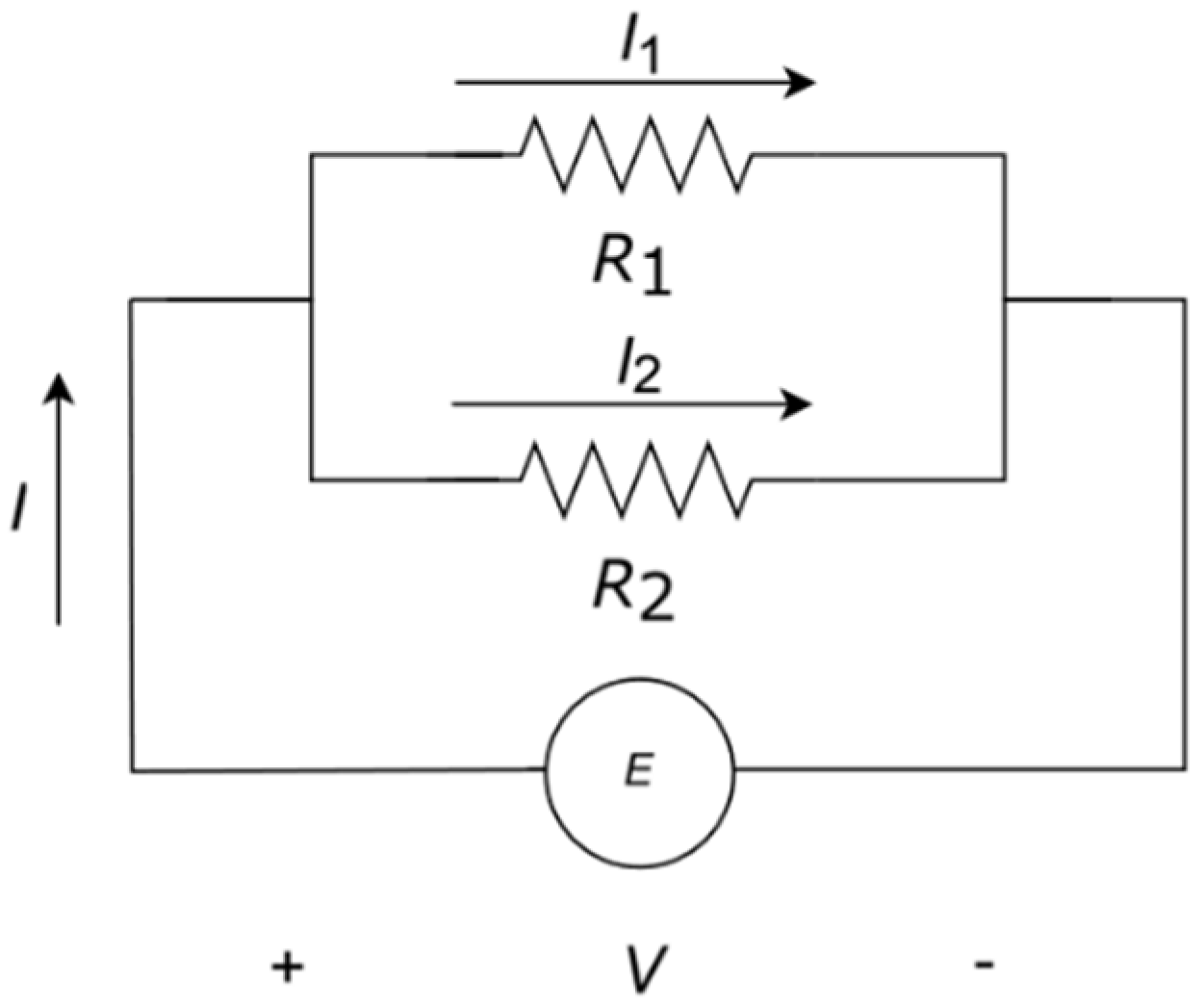
Figure 2.
Voltage divider with two resistors in series. E stands either for a voltage or current source.
Figure 2.
Voltage divider with two resistors in series. E stands either for a voltage or current source.
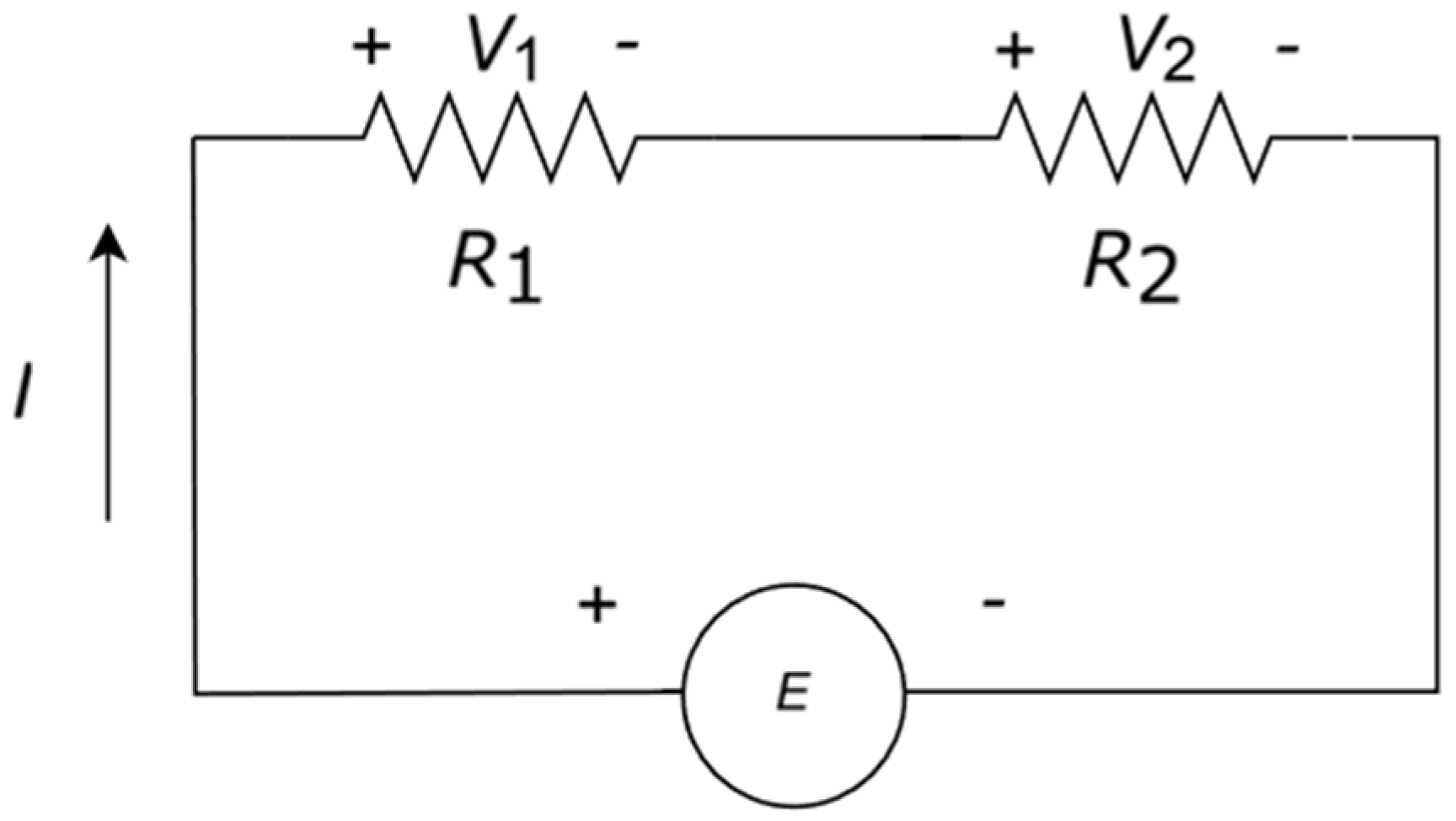
Figure 3.
Equivalent series resistance and capacitor with a power source E.
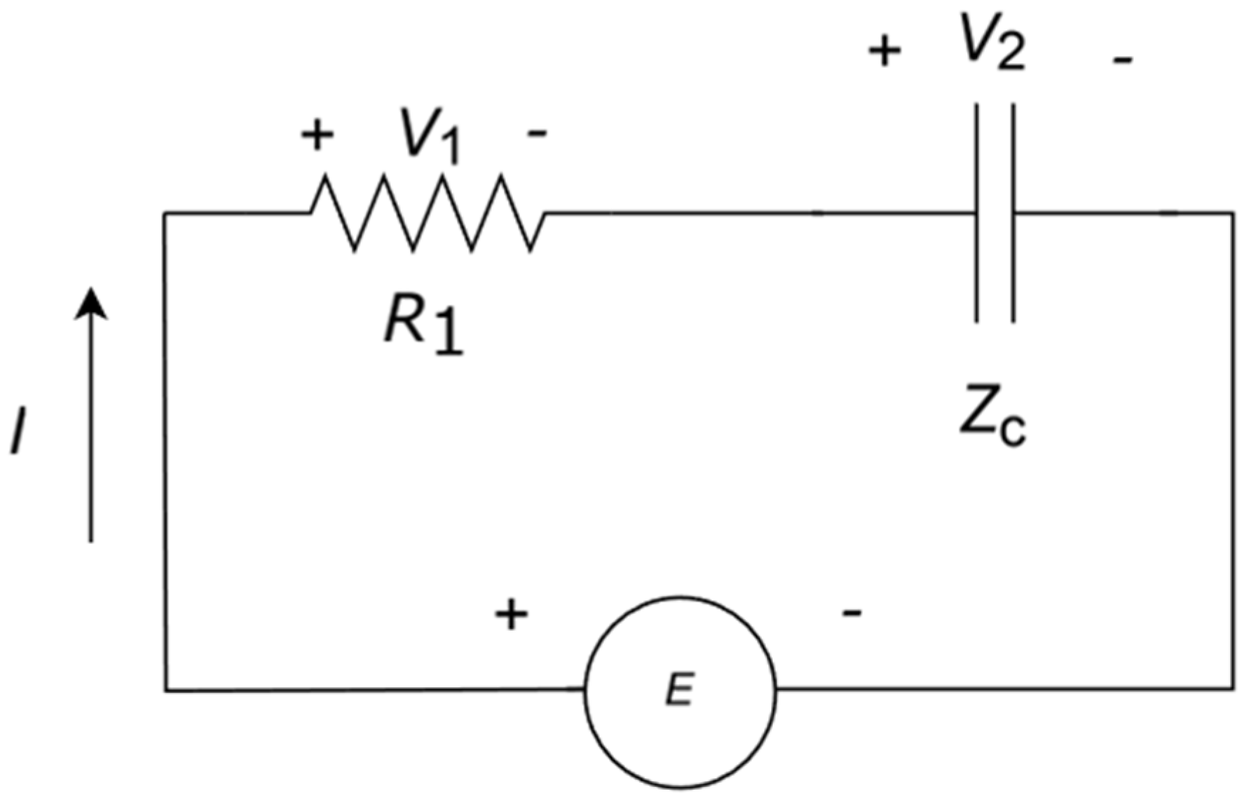
Figure 4.
Configurational entropy (left) and thermal entropy (right) as a function of the normalized resistor ratio for a current source of 1 A and integration time of 1 s. Sconfig maximum is 0.68 for equal resistors and evolve to 0 when the difference between resistors increases. Stherm increases with R2.
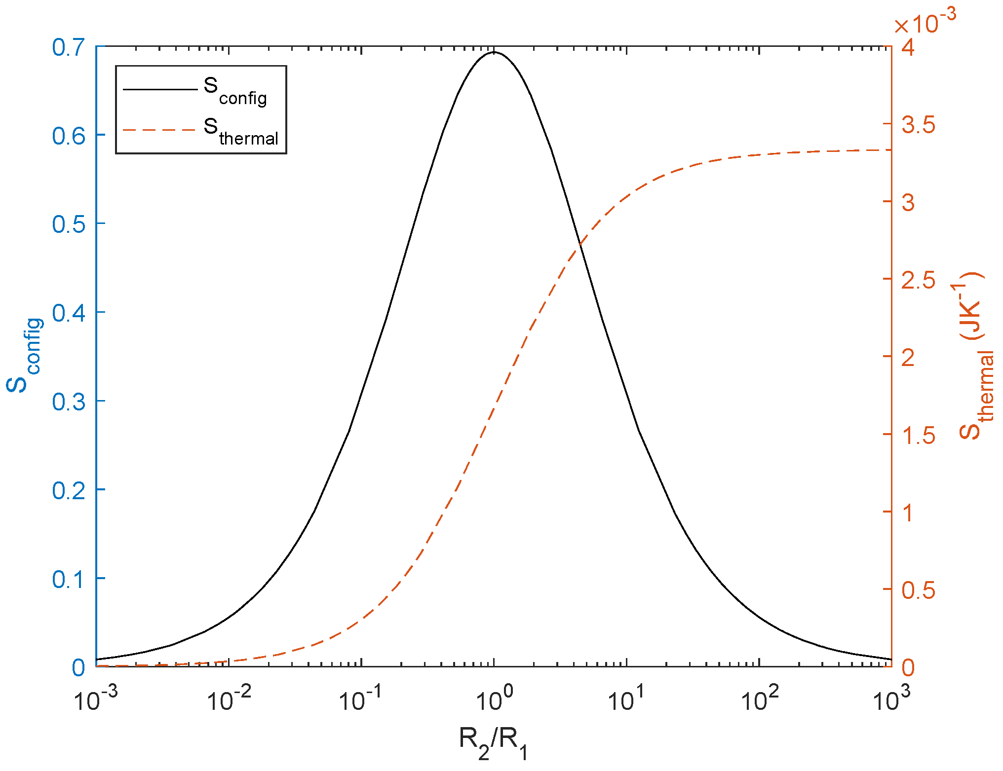
Figure 5.
Thermodynamic entropy vs. Configurational entropy from a normalized current source (1 A, in black) and normalized voltage source (1 V, in red) and integrated for 1 s.
Figure 5.
Thermodynamic entropy vs. Configurational entropy from a normalized current source (1 A, in black) and normalized voltage source (1 V, in red) and integrated for 1 s.
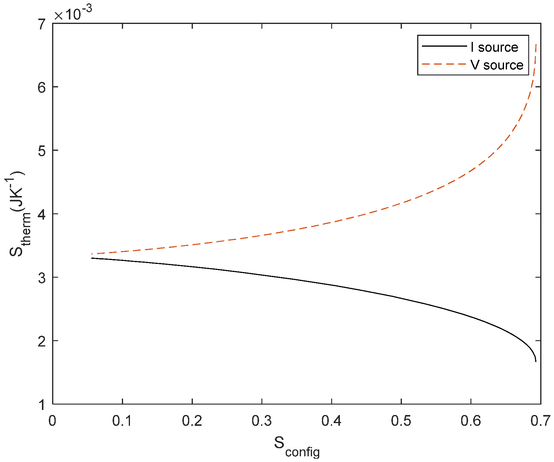
Figure 6.
Current through R2 for reference case (black), temperature-dependent resistor with α = 0.0040 (red), temperature-dependent resistor with α = -0.0005 (green) and temperature-independent resistors (blue). All cases considered T1 = 300 K and T2 = 400 K.
Figure 6.
Current through R2 for reference case (black), temperature-dependent resistor with α = 0.0040 (red), temperature-dependent resistor with α = -0.0005 (green) and temperature-independent resistors (blue). All cases considered T1 = 300 K and T2 = 400 K.
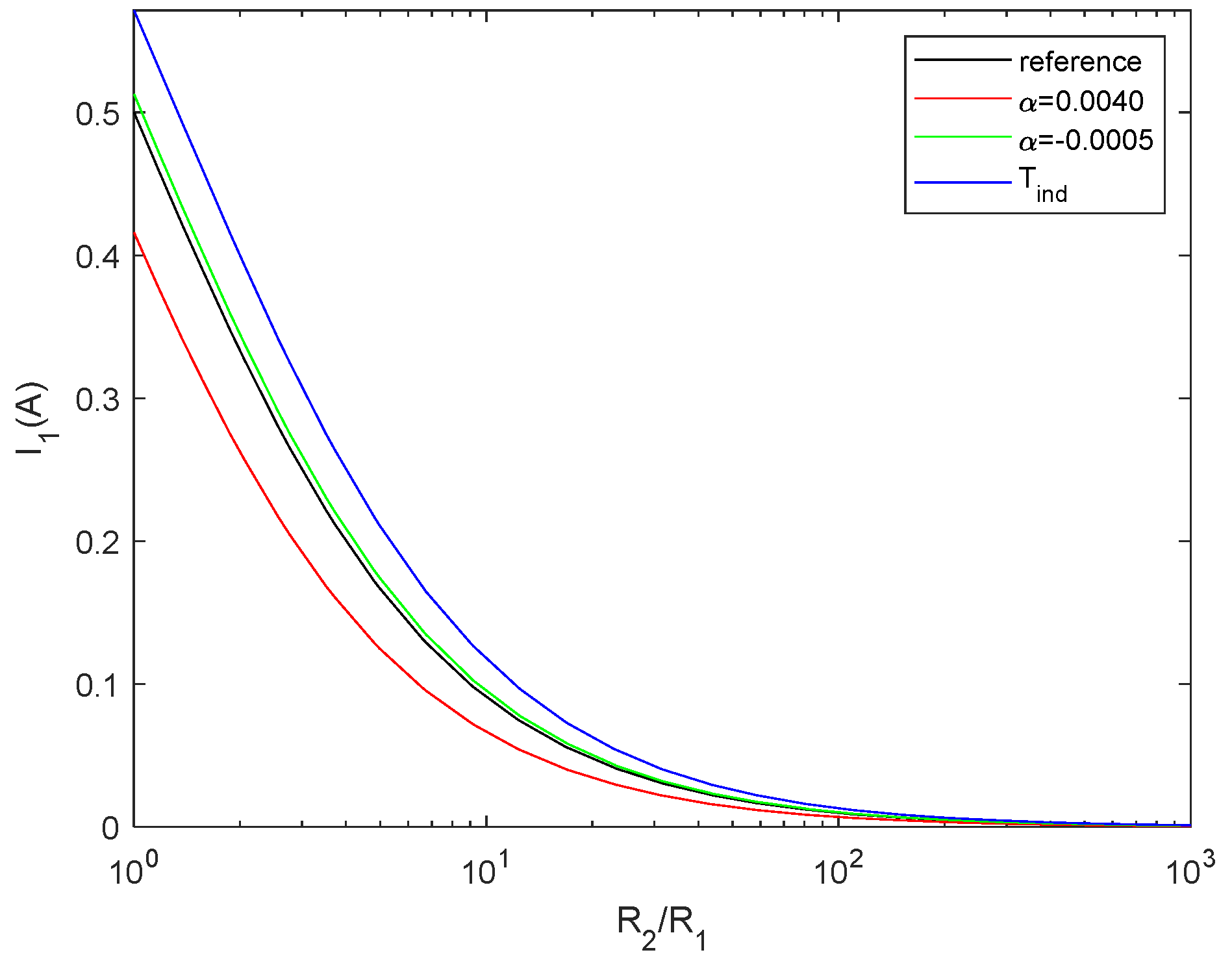
Figure 7.
Sconfig change due to resistance variation on temperature with α = 0.0040 (red) with respect to the reference configuration (black).
Figure 7.
Sconfig change due to resistance variation on temperature with α = 0.0040 (red) with respect to the reference configuration (black).
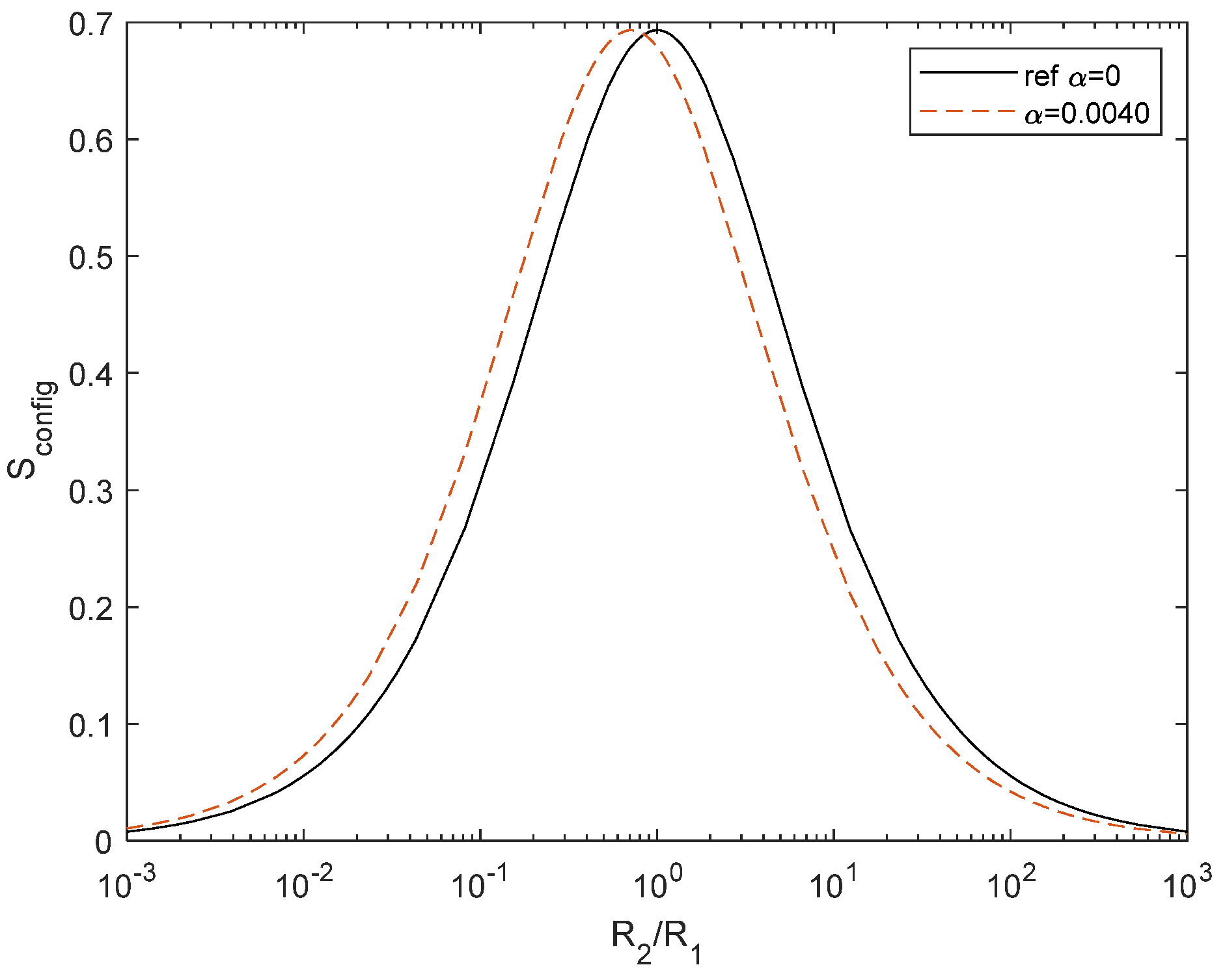
Figure 8.
Stherm for reference case (black) and for temperature-dependent resistor with α = 0.0040 (in red).
Figure 8.
Stherm for reference case (black) and for temperature-dependent resistor with α = 0.0040 (in red).
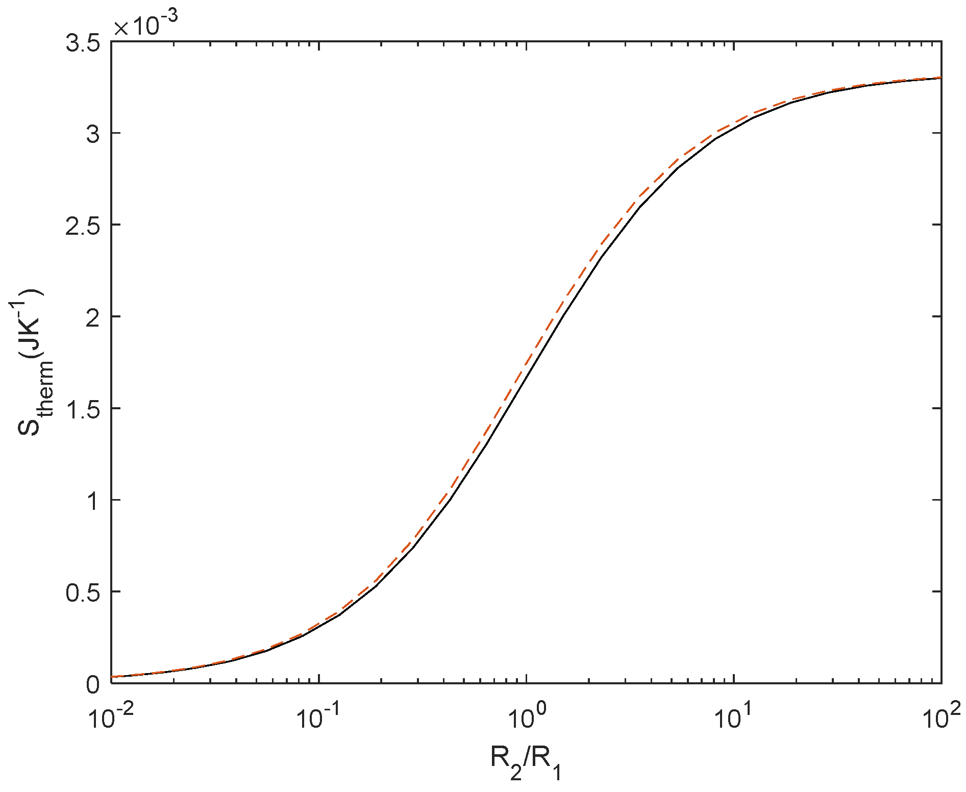
Figure 9.
Stherm as a function of Sconfig for reference configuration (black) and thermal-dependent resistor (red) with α = 0.0040 (red), α =-0.0005 (green) for a current source of 1 A. The difference between curves is related to the entropy change of the resistor.
Figure 9.
Stherm as a function of Sconfig for reference configuration (black) and thermal-dependent resistor (red) with α = 0.0040 (red), α =-0.0005 (green) for a current source of 1 A. The difference between curves is related to the entropy change of the resistor.
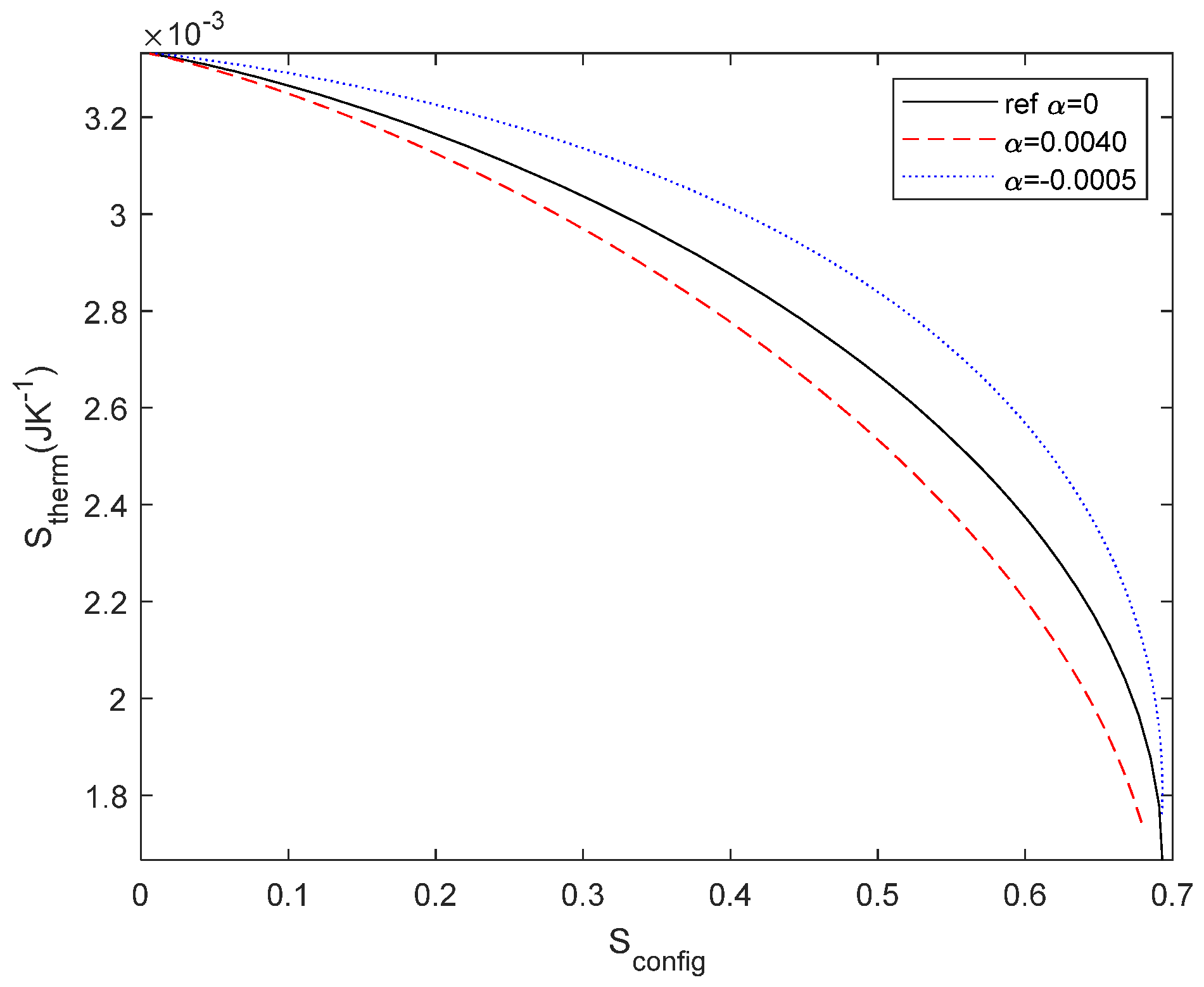
Figure 10.
Stherm as a function of Sconfig for current source (black) and voltage source (red) for series resistors. The red point of maximum Sconfig and maximum Stherm corresponds to R1 = R2 as described by the maximum power transfer theorem and pointed out with the arrow.
Figure 10.
Stherm as a function of Sconfig for current source (black) and voltage source (red) for series resistors. The red point of maximum Sconfig and maximum Stherm corresponds to R1 = R2 as described by the maximum power transfer theorem and pointed out with the arrow.
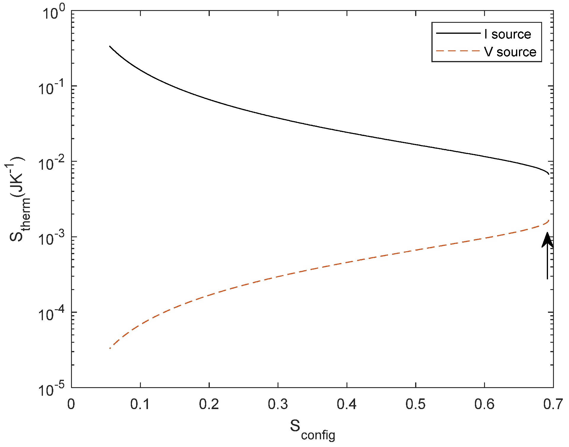
Figure 11.
Stherm as a function of Sconfig for reference configuration (black) and thermal-dependent resistor (red) with α = 0.0040 for a voltage source. The difference between both curves is related to the entropy change of the resistor.
Figure 11.
Stherm as a function of Sconfig for reference configuration (black) and thermal-dependent resistor (red) with α = 0.0040 for a voltage source. The difference between both curves is related to the entropy change of the resistor.
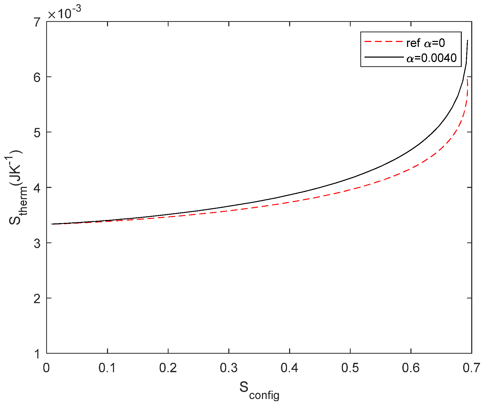
Figure 12.
(a) Tree shape network with three elements (b) Sconfig for 3 resistor circuit. R2 is variable and R3 = 1 Ω (black line) and R3=10 Ω (dashed red line). All other resistors are fixed to 1 Ω. (c) Stherm for the circuit with R3 = 1 Ω (black line) and R3=10 Ω (dashed red line) E = 1 V and (d) Sconfig and Stherm relationship with R3 = 1 Ω (black line) and R3=10 Ω (dashed red line), R2 as a variable and E = 1 V. R symmetry is lost when R3 and R1 are different. The arrows point at the maximum Sconfig.
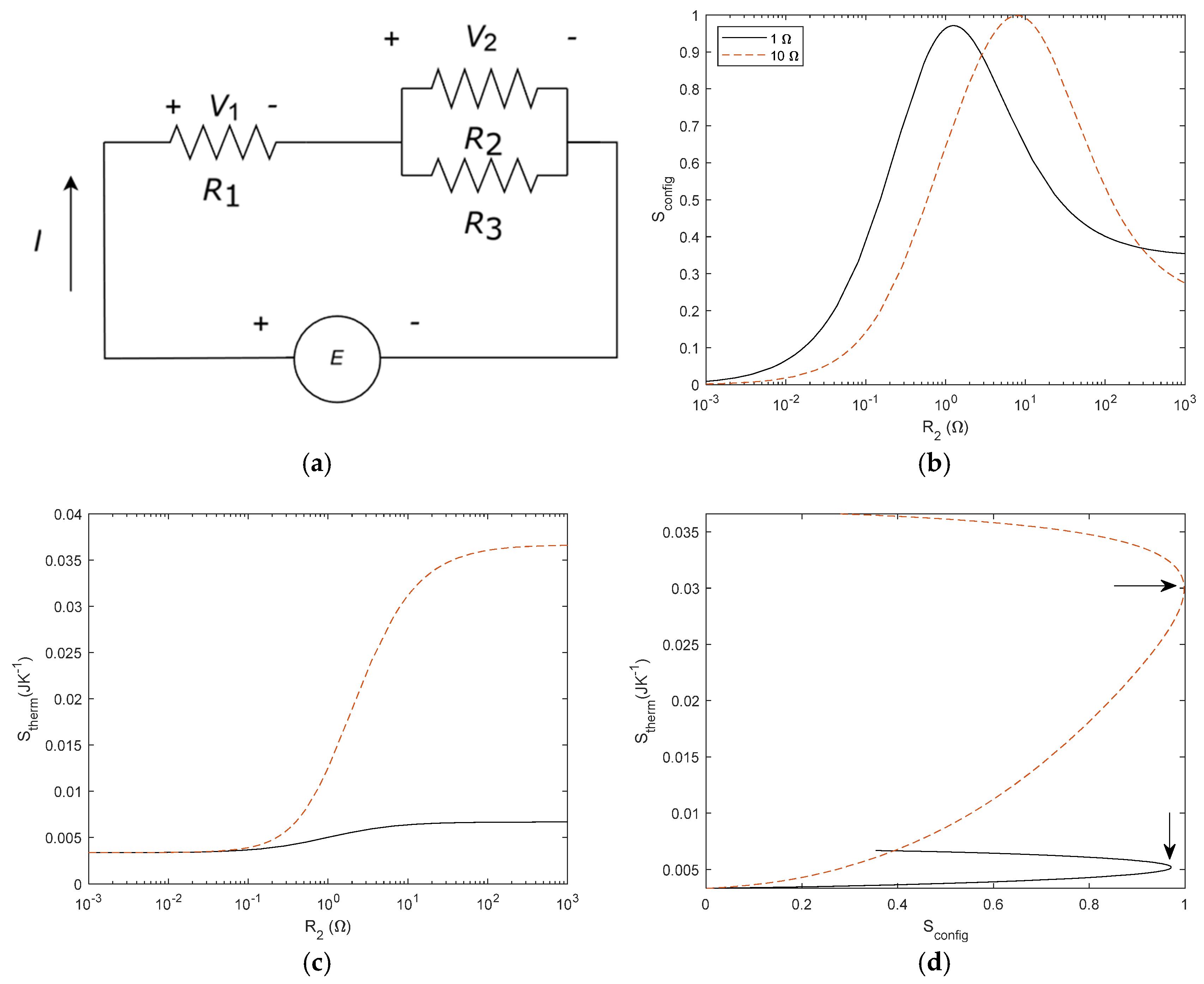
Figure 13.
(a) Tree shape network with seven elements (b) Sconfig for 7 resistor circuit. R2 is variable and R3 = 1 Ω (black line) and R3=10 Ω (dashed red line). All other resistors are fixed to 1 Ω. (c) Stherm for the circuit with R3 = 1 Ω (black line) and R3=10 Ω (dashed red line) E = 1 V and (d) Sconfig and Stherm relationship with R3 = 1 Ω (black line) and R3=10 Ω (dashed red line), R2 as a variable and E = 1 V. Symmetry is lost when R3 and R1 are different.
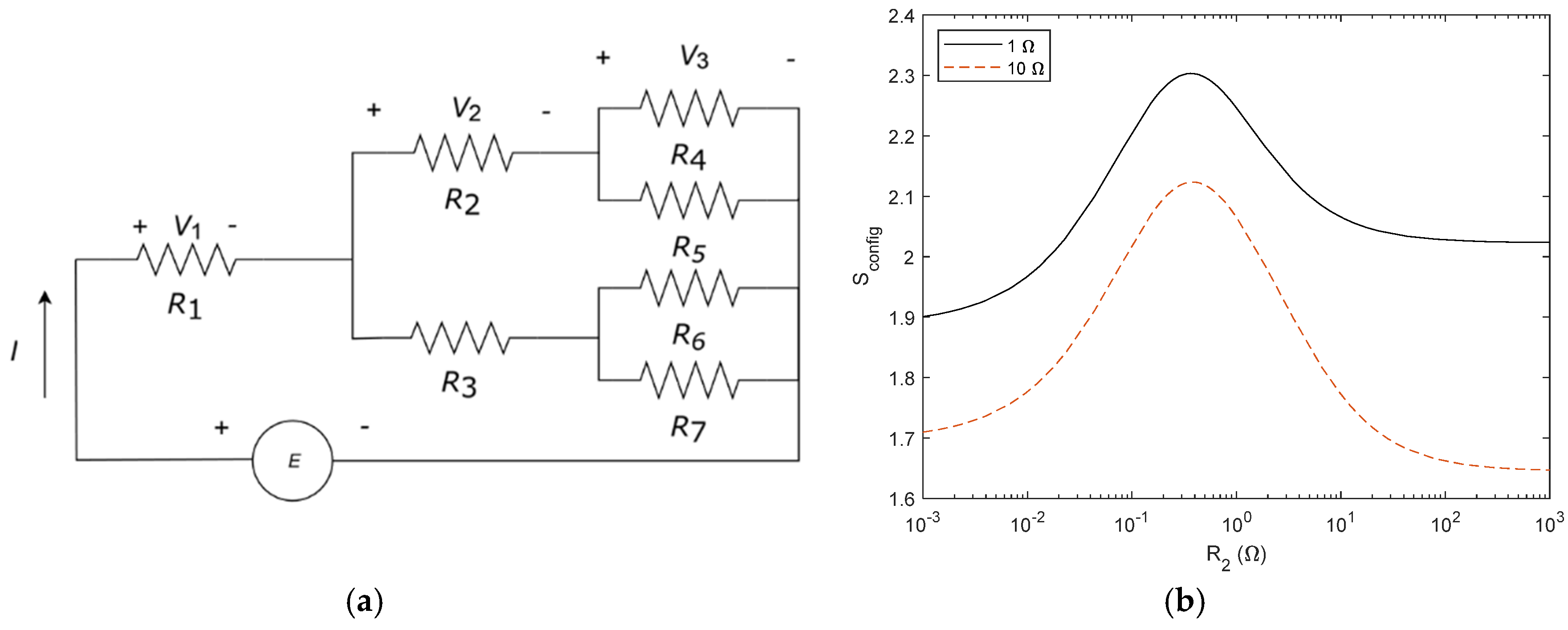
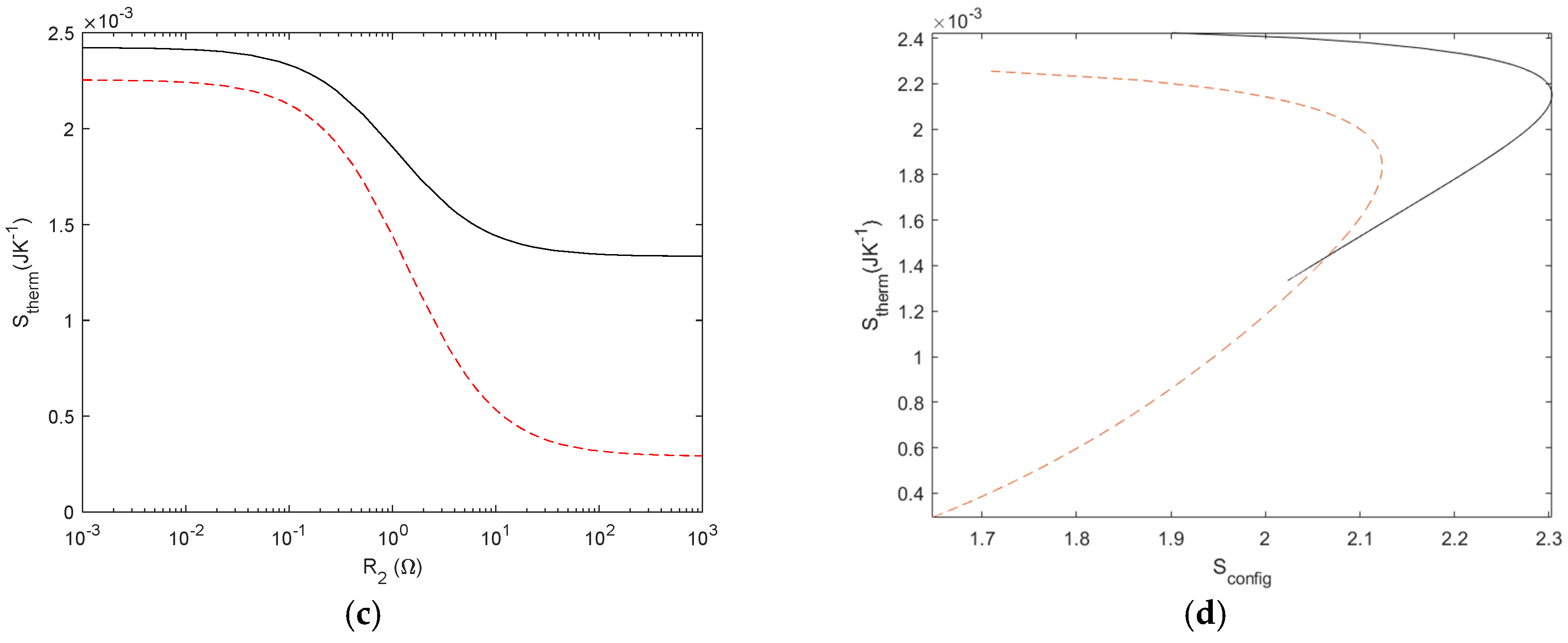
Figure 14.
Circuit with two voltage sources. In the figure, V2 is in series with R1. We simulated the cases V2 in series with R1 and in series with R2. Sconfig-Sthermal relationship for the reference circuit (V2 = 0) and two sources with V2 in series to R1 (red) and V2 in series to R1, as R2 is the swept variable.
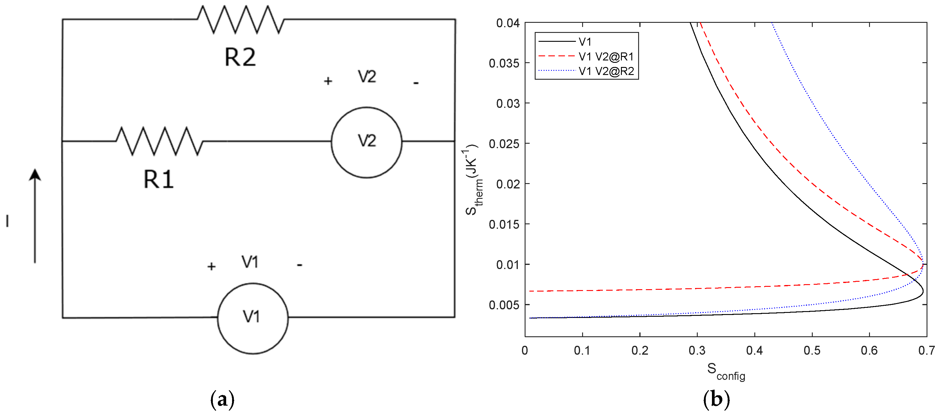
Figure 15.
– Modulus of Sconfig as a function of frequency for C = 1 F, R = 1 Ω (Black) and R= 10 Ω (red).
Figure 15.
– Modulus of Sconfig as a function of frequency for C = 1 F, R = 1 Ω (Black) and R= 10 Ω (red).
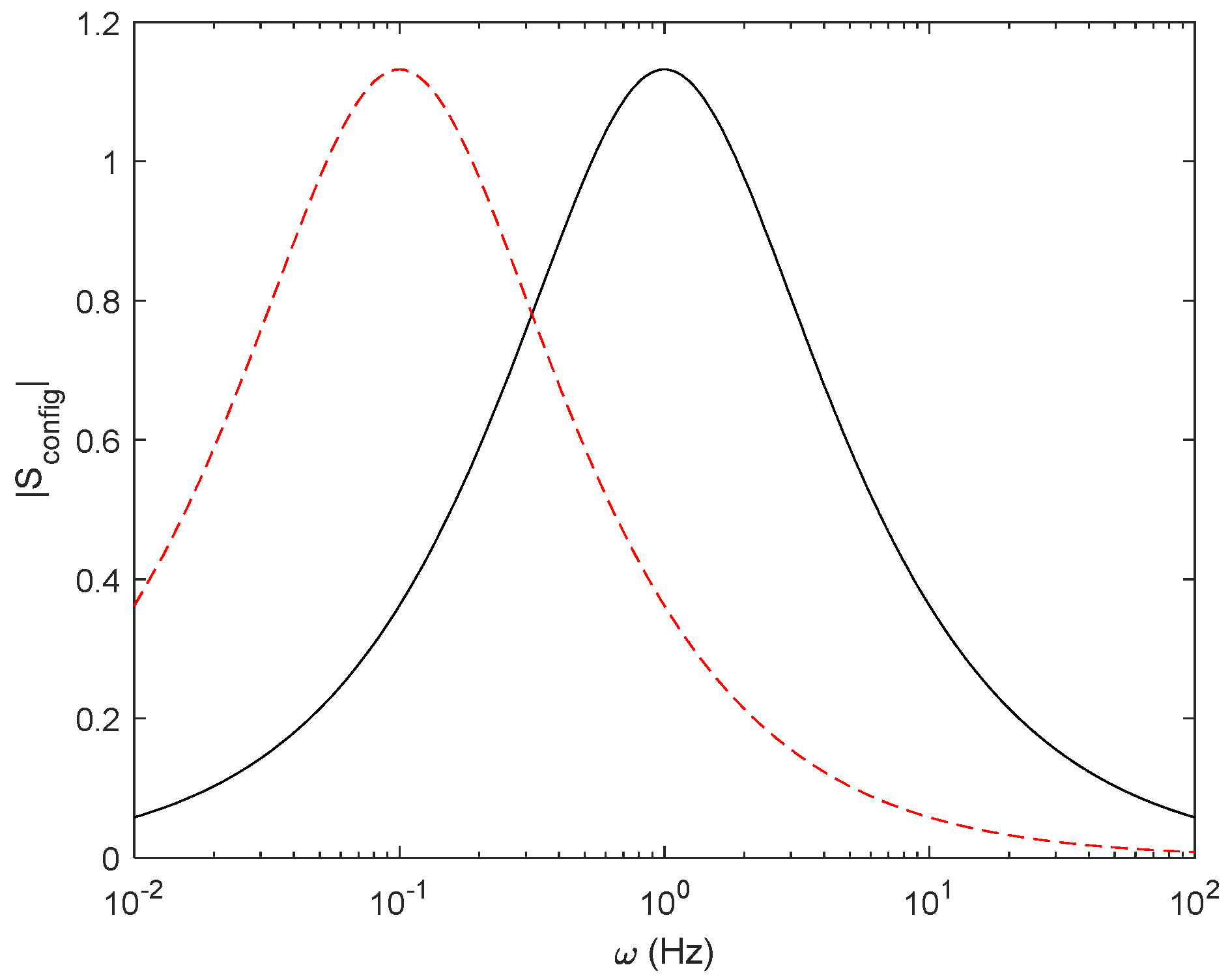
Figure 16.
Nyquist plot for Sconfig for R = 1 Ω, C = 1 F and 1 mHz < ω < 1 kHz.
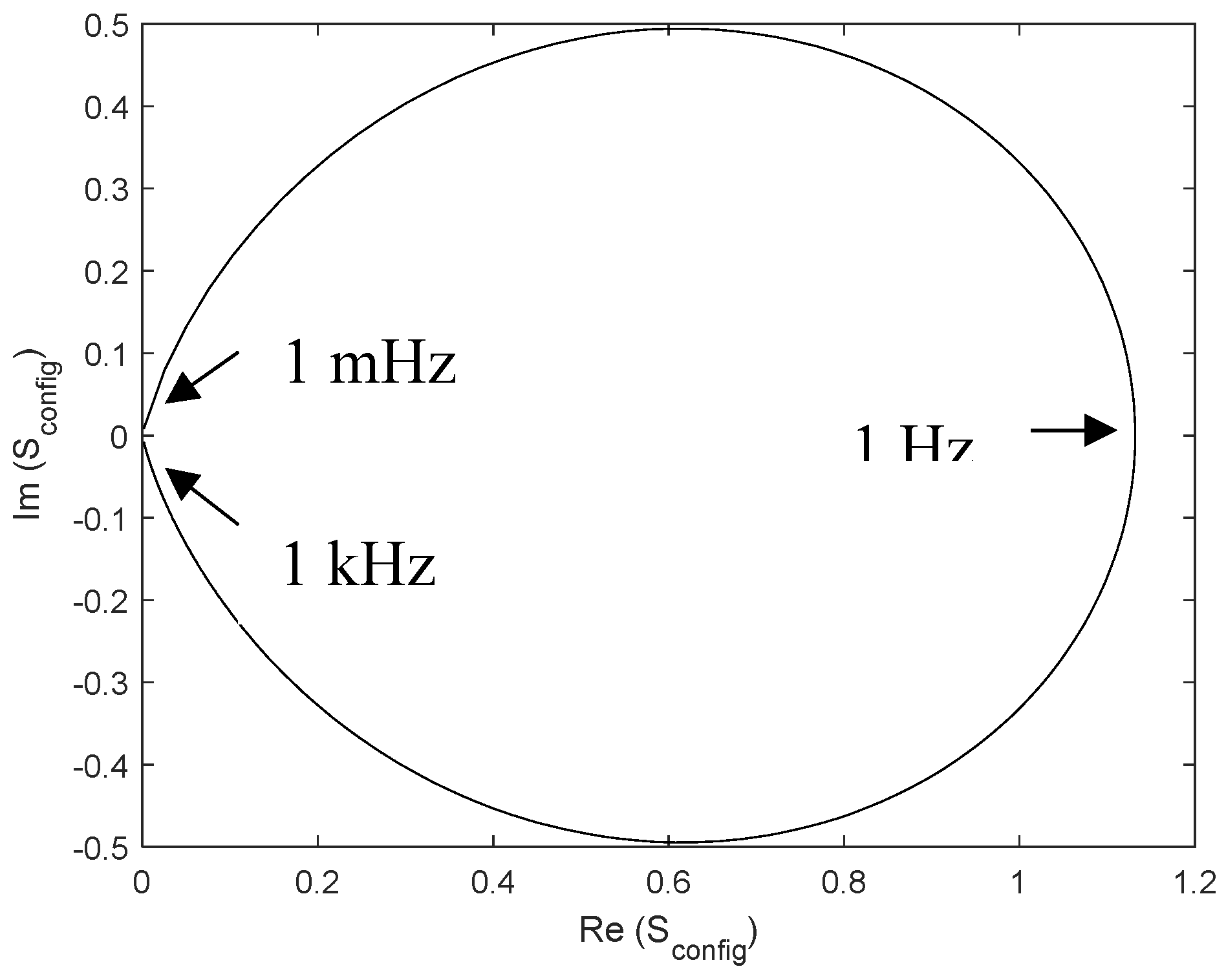
Figure 17.
– Relationship between Sconfig and Stherm for an R-C system (R = 1 Ω, C = 1 F and T = 300 K). A similar behaviour to resistor circuits is found, showing the generality of the method for linear systems.
Figure 17.
– Relationship between Sconfig and Stherm for an R-C system (R = 1 Ω, C = 1 F and T = 300 K). A similar behaviour to resistor circuits is found, showing the generality of the method for linear systems.
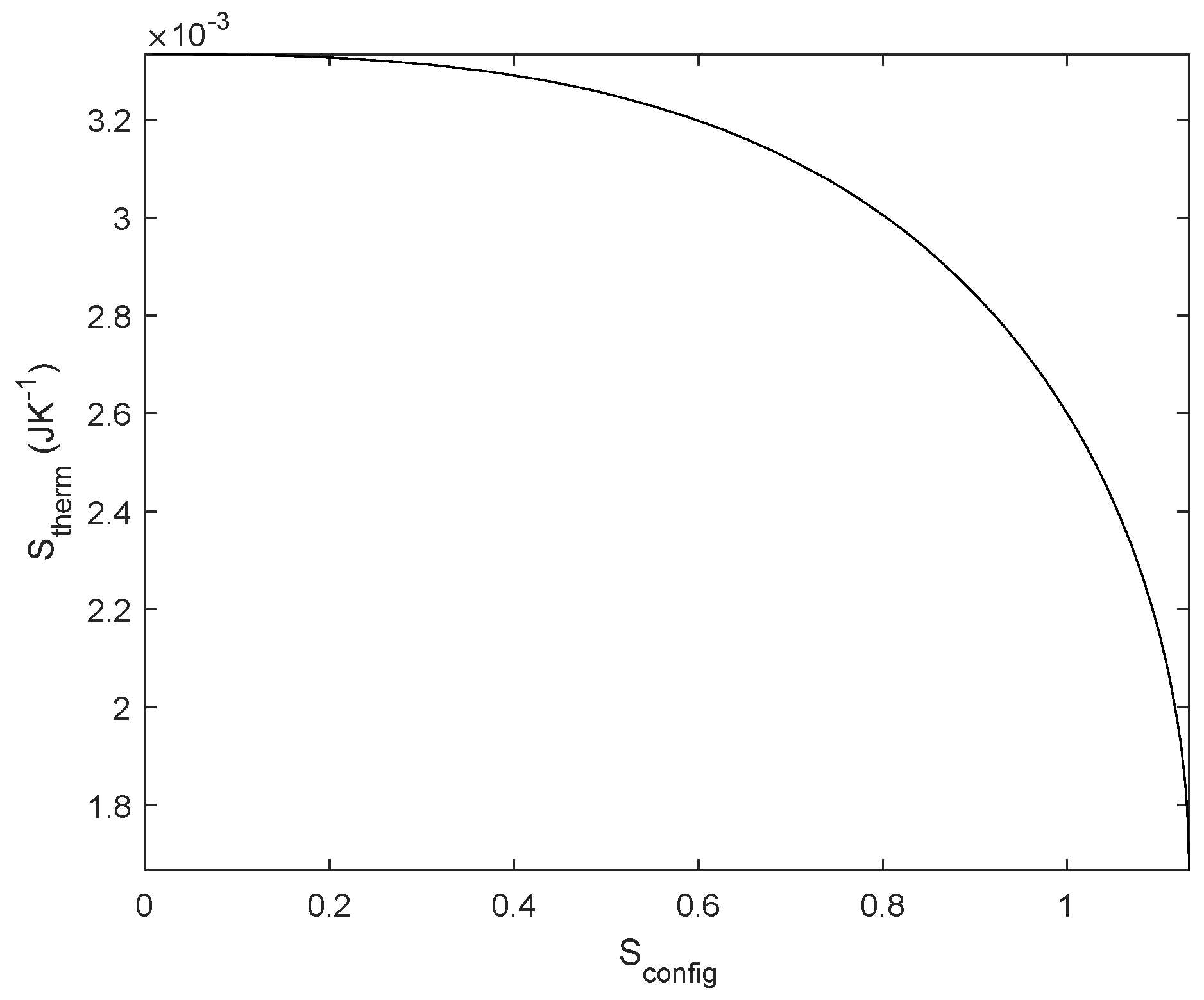
Figure 18.
Time dependent profiles for degradation in a parallel R1//R2 circuit with R1 = 1 Ω, T=300 K and I = 1 A. (a) time evolution of resistor degradation according to Equations (22)–(24) (b) Time dependent evolution of Sconfig (c) Time dependent evolution of Sthermal (d) relationship between Sconfig- Sthermal and (e) relationship between Sconfig and
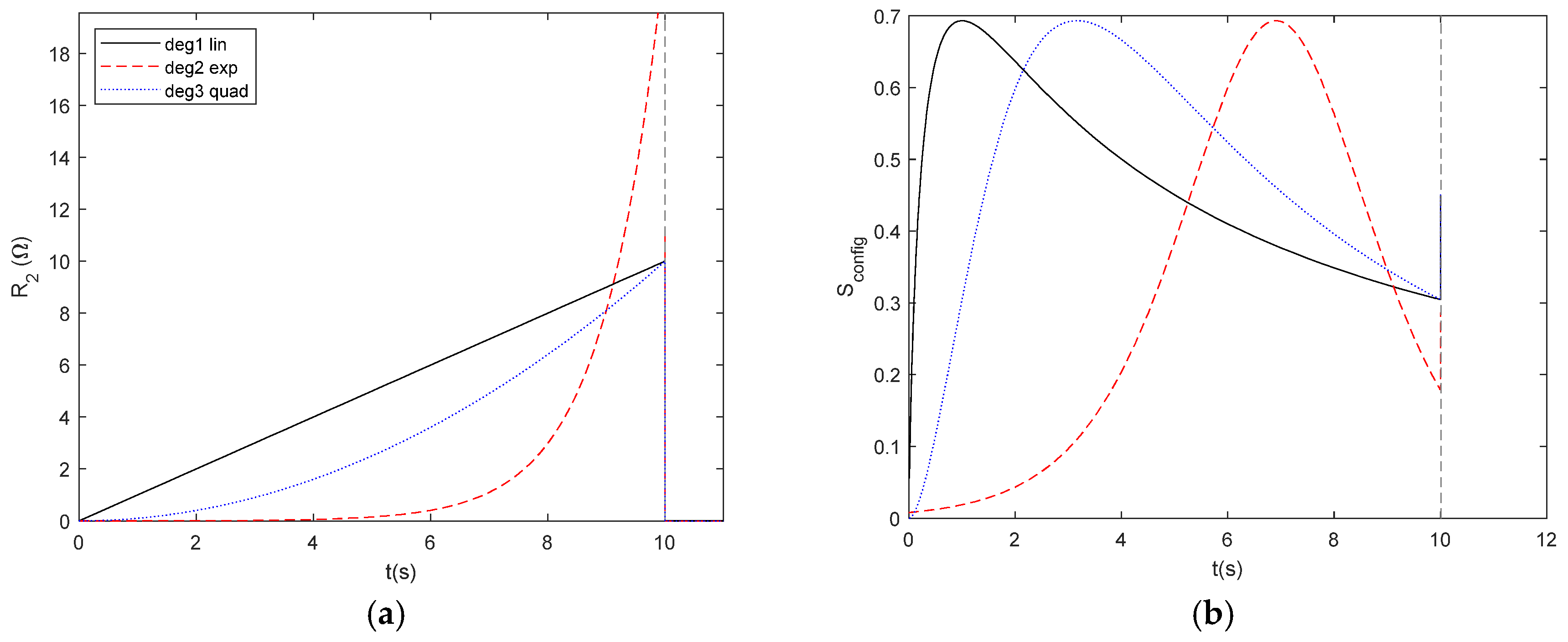
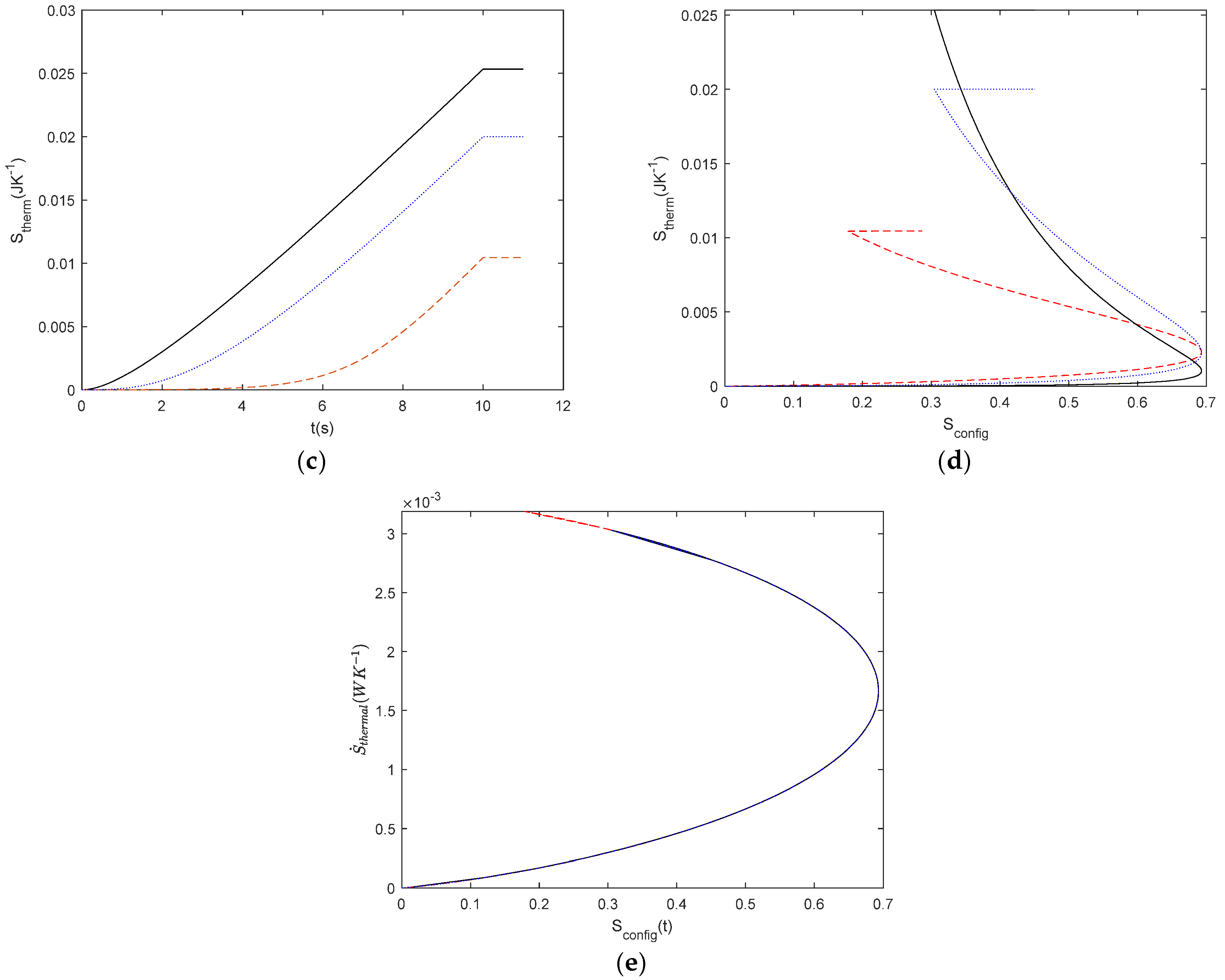
Figure 19.
– Relationship between Stherm – Sconfig. It is same data of Figure 18 (d) with the axis exchanged.
Figure 19.
– Relationship between Stherm – Sconfig. It is same data of Figure 18 (d) with the axis exchanged.
Disclaimer/Publisher’s Note: The statements, opinions and data contained in all publications are solely those of the individual author(s) and contributor(s) and not of MDPI and/or the editor(s). MDPI and/or the editor(s) disclaim responsibility for any injury to people or property resulting from any ideas, methods, instructions or products referred to in the content. |
© 2024 by the authors. Licensee MDPI, Basel, Switzerland. This article is an open access article distributed under the terms and conditions of the Creative Commons Attribution (CC BY) license (http://creativecommons.org/licenses/by/4.0/).
Copyright: This open access article is published under a Creative Commons CC BY 4.0 license, which permit the free download, distribution, and reuse, provided that the author and preprint are cited in any reuse.


