
Submitted:
02 January 2024
Posted:
03 January 2024
You are already at the latest version
Abstract
Generalized distributions have been studied a lot recently because of their flexibility and relia-bility in modeling lifetime data. The two-parameter exponentially-modified logistic distribution is a new flexible modified distribution that was introduced recently. It is regarded as a strong competitor for widely used classical symmetrical and non-symmetrical distributions such as normal, logistic, lognormal, and log-logistic. In this study, the unknown parameters of the dis-tribution are estimated using the maximum likelihood method. The Grey Wolf Optimization al-gorithm, which is a new meta-heuristic algorithm, is applied in order to solve the nonlinear like-lihood equations of the study model. The performance of the Grey Wolf Optimization method is compared to that of the other meta-heuristic algorithms used in this study, which include the Whale Optimization Algorithm, the Sine Cosine Algorithm, and the Particle Swarm Optimiza-tion Algorithm. The efficiencies of maximum likelihood estimates for all algorithms are com-pared via an extensive Monte-Carlo simulation study. The likelihood estimates for the location α and scale β parameters of the exponentially-modified logistic distribution developed with the Grey Wolf Optimization algorithm are the most efficient among others, according to simulation findings. Four real datasets are analyzed to show the flexibility of this distribution.
Keywords:
maximum likelihood
; exponentially‐modified logistic distribution
; Grey Wolf optimization
; swarm intelligence
; Monte Carlo simulation
1. Introduction
The two-parameter exponentially-modified logistic distribution is one of the new distributions that have been generalized recently. It is a distribution with more flexibility than other similar distributions for fitting data in many scientific fields, such as biological and psychological evolution, energy resource prediction, and technological and economic diffusion. Practically, it can be considered a better alternative than symmetrical distributions such as the logistic and normal distributions, as well as many other non-symmetrical statistical distributions in different application cases, especially when a little skewness exists. This can be viewed as this distribution’s main contribution. The generalization of this distribution has emerged from the importance of logistic and exponential distributions, which have both been combined to form a new, more reliable distribution called the two-parameter exponentially-modified logistic distribution. Reyes et al. first presented this distribution in 2018 [1]. The logistic distribution is recognized to be similar to the normal distribution; they are both members of the location-scale family, but the difference is that the logistic distribution has heavier tails [2]. The importance of logistic distribution is that it has the ability to be used in many scientific areas like physical science, finance, and many applications in reliability and survival analysis, besides the major utility of its distribution function in logistic regression, logit models, and neural networks [3]. More properties and details about logistic distribution are available in [4,5]. On the other hand, the exponential distribution, which is concerned with the measurement of time needed until the occurrence of a specific event [3], previously was the basis of reliability and life expectancy evaluation for many lifetime data distributions, but in further research in reliability theory, it was revealed that modeling by the exponential distribution is only useful for the first approximation and can’t be enough for a lot of problems in many cases. More details about the exponential distribution can be found in [6]. In the last two decades, in order to give better-fitting solutions and increase fit effectiveness for model functions that have no closed-form and require a numerical method in lifetime data analysis, many generalizations and modified extensions of the exponential distribution have been suggested to become more flexible and capable for modeling real-world data, especially when the characteristics of classical distributions are limited and, practically, they cannot provide a good fit in many situations [3,7,8,9,10]. Various exponentiated distributions have been generalized; for instance, in 1998, the exponentiated exponential (EE) distribution was first introduced by Gupta & Kundu [11] and is considered the first extension of the exponential distribution family. The exponentiated Weibull (EW) distribution was discovered in 2006 by Pal et al. [12], the exponentiated Gamma (EG) distribution was generalized in 2007 by Nadarajah & Gupta [13], another extension was proposed in 2011 by Nadarajah & Haghighi [14], the exponentiated log-logistic (ELL) distribution with two parameters was discovered in 2019 by Chaudhary [15], and many other well-known distributions recently have been extended and modified by the exponential distribution family. In general, there are many different statistical methodologies for estimating the parameters of any distribution, such as the maximum likelihood (ML) method, the Method of Moments (MOM), the Least Squares (LS) method, the Bayes method, and so forth. ML is the most widely used methodology among all statistical methods because of its high performance and well-known asymptotic properties for parameter estimators such as bias, consistency, efficiency, and so forth in comparison with any other method [16]. The basic principle of the ML methodology is to find the estimator values for the parameters of concern that maximize the likelihood function of the model, but in most cases, an explicit solution is rarely available because of the presence of nonlinear functions. Therefore, iterative algorithms to maximize the likelihood function are needed [17].
The primary goal of this research is to choose the best algorithm for calculating the maximum likelihood estimation of the location α and scale β parameters of the exponentially-modified logistic distribution and to show the applicability of this distribution in many areas. However, for the two-parameter exponentially-modified logistic distribution, explicit solutions to the likelihood equations were not found, and this is the main problem highlighted by this study. To solve this problem, ML estimates are found through the use of iterative numerical techniques based on traditional or non-traditional algorithms. In general, the Newton method is a common type of traditional iterative technique that is commonly used to solve the equation system generated by partial derivatives of the likelihood function to find estimated values of the parameter of interest for statistical distributions, but its major drawback is that it uses a gradient-based search algorithm to find the best parameter values based on the inverse of the hessian matrix, making it only applicable to functions that can be differentiated at least twice. At the same time, to stay in the same category and avoid such limitations, another type of traditional iterative techniques based on direct search algorithms without any need for the gradient information of the likelihood function can be used, such as the Nelder Mead (NM) algorithm. However, all traditional numerical algorithms start from a randomly selected initial guess and move towards the optimum solution iteratively, with no guarantee that the final solution is globally optimal. Besides that, the gradient-based methods can’t be used for discontinuous functions. Moreover, the final solution may get stuck at local optimum points, and the global optimum may never be reached [18]. To avoid such drawbacks, the use of non-traditional algorithms like meta-heuristic algorithms is preferable and recommended for solving complex problems, especially when traditional algorithms fail. At the same time, meta-heuristic algorithms guarantee global convergence with more simplicity, flexibility, and a derivation-free mechanism [19]. A variety of meta-heuristic algorithms have been applied in the ML method for estimating the parameters of many statistical distributions and models, such as in [20,21,22,23,24]. Among the heuristic algorithms, Particle Swarm Optimization (PSO), a well-known algorithm used in many fields [25], and new algorithms distinguished by their simplicity, flexibility, ease of implementation, and lower number of required parameters, such as the Grey Wolf Optimization (GWO) [26], the Whale Optimization Algorithm (WOA) [27], have proven to be dependable in solving real optimization problems where the objective function is nonlinear. In particular, many studies, including [28,29,30,31], considered the PSO algorithm for estimating the distribution parameters. In [32], GWO is applied for the estimation of three parameters of a new statistical distribution named the Marshall Olkin Topp Leon exponential distribution. Wang et al. [33] applied three meta-heuristic algorithms, including the GWO, PSO, and cuckoo search algorithms (CSA), and four numerical methods. The outcomes of the experimental work show that the GWO gives the most accurate and efficient results for estimating the parameters of the Weibull distribution, which is the best distribution in comparison with another distribution fitting wind energy data. Wadi [34] estimated the parameters of five statistical distributions, including Rayleigh, Weibull, Gamma, Burr Type XII, and generalized extreme value distributions, by using the ML method based on two heuristic algorithms: GWO and WOA. The results showed that the Gamma distribution based on GWO and WOA outperformed other distributions in modeling wind speed data and that GWO was more robust and faster than WOA. Furthermore, Wadi and Elmasry [35] added three more metaheuristic optimization algorithms to GWO and WOA, namely the Grasshopper Optimization Algorithm (GOA), Moth-Flame Optimization (MFO), and Salp Swarm Algorithm (SSA), which are used for estimating the parameters of the same distributions as Rayleigh and Weibull as well as other distributions such as inverse Gaussian, Burr Type XII, and Generalized Pareto to describe different wind speed data. According to the performance criteria, the Weibull distribution based on GWO, WOA, and MFO has the best goodness of fit. Al-Mhairat and Al-Quraan [36] estimated distribution parameters for Weibull, Rayleigh, and Gamma distributions by using the ML method based on three heuristic algorithms, which are PSO, GWO, and WOA, by implementing wind speed data. According to the performance indicators, such as root mean square error (RMSE) and coefficient of determination (R2), the gamma distribution based on the PSO algorithm achieved the best results, but if the mean absolute error (MAE) indicator is considered, then the method based on the GWO algorithm provides the best results. The sine-cosine algorithm (SCA) [37] is another simple, flexible, and easy-to-implement heuristic algorithm with a small number of required parameters. It is used for solving many optimization problems in various scientific areas, such as [38,39,40]. However, it has never previously been used to estimate the parameters of a statistical distribution. It can therefore be applied to the ML method to see whether or not implementing it to estimate location and scale parameters for the two-parameter exponentially-modified logistic distribution will produce better outcomes due to the features mentioned above. This paper’s contribution is to employ and examine these four meta-heuristic optimization algorithms by applying the ML method to obtain the estimator’s values for the location and scale parameters of the two-parameter exponentially-modified logistic distribution based on the GWO, WOA, SCA, and PSO algorithms, then comparing and evaluating their performances by conducting an extensive Monte-Carlo simulation study. To best of our knowledge, this is the first study to obtain the ML estimators for the location α and scale β parameters of the two-parameter exponentially-modified logistic distribution by using various meta-heuristic algorithms.
The following is how the rest of the article is organized: In Section 2, the two-parameter exponentially-modified logistic distribution and its properties are presented. In Section 3, the ML estimation methodology for GWO and the other numerical techniques based on other meta-heuristic algorithms used in this study are introduced. In Section 4, the efficiencies of the parameter estimators are compared via a comprehensive Monte-Carlo simulation study. Four applications of real datasets are implemented in Section 5. In the final section, the study ends with some conclusions.
2. Materials and Methods
2.1. Two-Parameter Exponentially-Modified Logistic Distribution
The generalization of this distribution is made by the combination of a logistic distribution with parameters for location α and scale β and the same scale parameter for the exponential distribution. As a result, the two-parameter exponentially modified logistic distribution is produced, with the left tail influenced by exponential distribution and the right tail distributed by logistic distribution. For the sake of simplicity, in the remaining portion of the study, this distribution will be denoted by "EMLOG" distribution.
If X is a random variable with a parameterized location α and scale β that follows an EMLOG distribution, X∼ EMLOG (α, β), then the probability density function (pdf) of X is:
X’s cumulative distribution function (cdf) seems to be as follows:
See the EMLOG distribution in Figure 1, where the plots of the EMLOG distribution are illustrated for certain values of α and β. The general formula for the EMLOG distribution’s kth moment (μk) expression (for k = 1,2,3, ⋯) is:
where Bn and Γ(.) refer to Bernoulli numbers and the Gamma function, respectively. The mean, variance, skewness (γ1), and kurtosis (γ2) values of the random variable X are computed using formula (3), see [1].
2.2. Maximum Likelihood Estimation
The ML estimation for the parameters of interest are the values in the parameter space that maximize the likelihood function; in most cases, for calculation simplicity, the likelihood function’s logarithm is used. In this study, the log-likelihood (ln L) function is given below for estimating the unknown parameters α and β for the EMLOG distribution.
where zi=(xi-α)/β. In order to estimate the likelihood parameters for the ln L function for the EMLOG distribution, the partial derivatives with respect to the parameters of interest are taken and equated to zero. The likelihood equations are given as shown below.
and
As we can see from Equations (9) and (10), they have nonlinear functions, and an explicit solution for the likelihood equations cannot be obtained. Therefore, iterative algorithms are needed to solve these equations and obtain ML estimates for the location and scale. In this study, GWO, WOA, SCA, and PSO are some effective and powerful meta-heuristic algorithms considered as numerical techniques for estimating the likelihood estimators for the EMLOG distribution, and they are briefly introduced in the next few subsections.
2.2.1. Grey Wolf Optimization (GWO)
The GWO is a new intelligent method that is obtained from swarms based on meta-heuristic techniques that were modeled by the grey wolf leadership hierarchy in the process of trapping and hunting prey in nature. Mirjalili et al. made the first proposal in 2014 [26]. GWO has become a widely known critical device in swarm intelligence for optimization in almost all areas, such as engineering, physics, and many other applications in various scientific fields [41]. GWO is a straightforward population-based probabilistic algorithm motivated by the hunting and socialization of grey wolves. According to the swarm intelligence categorization, it is classified as the only algorithm for solving continuous real-life optimization problems that relies on a leadership hierarchy [42]. For the hunting process, the groups of grey wolves are categorized into four types to compose hierarchical commands. These types are called alpha (α), beta (β), delta (δ), and omega (ω), in that order. Figure 2 shows this hierarchy.
At the first level of the hierarchy, type alpha (α) represents the dominant gray wolf that makes decisions and gives orders to the other wolves in the pack. Type beta (β) represents the gray wolf that helps the alpha (α) type in making decisions and observing the movements of other wolves at the next level of the hierarchal chain. A group of alpha types will be replaced by beta types when a group of alphas dies or becomes older. Types delta (δ) and omega (ω) are the third and fourth types of gray wolves, respectively. For sure, the delta (δ) wolf type dominates the omega (ω) wolf type, and both of them represent the lowest level in the hierarchy; they are allowed to eat after the alpha (α) and beta (β) types have finished eating [43,44]. Figure 3 depicts a flow diagram of the GWO.
The GWO algorithm consists of three main phases, which are: 1) searching; 2) encircling; and 3) hunting the prey. They are summarized as follows:
For the first iteration, randomly assign the positions of the N number of wolves as well as the GWO parameters for the mathematical modeling as follows:
- Control parameter (a), which is an important parameter that declines linearly for each iteration in the range [0,2] used in this algorithm. This parameter can indeed be determined using the formula:where the iteration in progress (current) and the entire number of iterations are denoted by t and Tmax, respectively.
- The coefficient vectors, A and C, can be found using the following formulas:where r1 and r2 are arbitrary vectors ranging from [0,1].
- Calculate the fitness value of each wolf type according to the fitness function, which is the same as the objective function represented by the ln L function in this study, and this fitness value refers to each wolf’s site in the pack. The highest value of the fitness function is considered the best position and assigned to the wolf of type alpha (α). The second and third highest fitness values are assigned to beta (β) and delta (δ) types of wolves, respectively. Steps 1 and 2 represent the searching phase of GWO.
- Update the position of each wolf in the pack surrounding the prey by calculating the distance between the current location (denoted by D) and the next location (denoted by) using the equations below.where is the current position vector at iteration t and Xp(t) is the best solution’s position vector (optimal) when iterating to the tth time. This step represents the phase of encircling behavior.
- Calculate the average value of the first three best solutions that refer to alpha (α), beta (β), and delta (δ) types of wolves because they have the best positions in the population. Besides that, they have the best knowledge of the prey’s potential location, which forces and obliges all the other wolves, including omega (ω), to change their current positions toward the best position, which has been determined by the following equations:whereand
The fitness value of the new position is calculated, and according to that, the wolves’ alpha (α), beta (β), and delta (δ) types are updated. This step represents the hunting phase. The attack happens with respect to the changing value of the coefficient vector A, which depends on the parameter (a) and decreases from 2 to 0 for each iteration step while the algorithm is working. Therefore, A is a value generated randomly within the interval [-2a, 2a]. If |A| < 1, the wolves are ready to attack the prey. Otherwise, the wolves are forced to diverge to explore a better location.
- 4.
- Finally, go back to step 3 to continue iteration until the convergence is satisfied by reaching the stopping criterion and the needed number of maximum iterations to overall acquire the most appropriate (optimal) solution. The solution values are called the GWO estimates of the parameters.
2.2.2. Whale Optimization Algorithm (WOA)
The WOA is also a unique swarm-based intelligent meta-heuristic methodology, recommended in 2016 by Mirjalili as well as Lewis for continuous optimization problems [27]. The inspiration for this algorithm has come from mimicking the hunting behavior of a specific type of whale (called a humpback) that applies a hunting strategy called the bubble-net feeding technique by creating bubbles along a circle around the prey, then slowly shrinking, encircling, and approaching the prey in a spiral shape through random search concerning each search agent’s location until finally, the hunt is complete [47,48,49].
WOA algorithm steps: [49]
The algorithm has three main phases that are: 1) encircling; 2) attacking by using the bubble net method, which includes shrinking encircling besides the mechanisms for spiral position updating; and 3) searching to catch prey. The steps are listed below.
- Initialize the position of the whale population randomly in the search space for the first iteration.
- Initiate the WOA parameters (a), A, and C, which are similar to GWO parameters previously calculated by Equations (11), (12), and (13), respectively, as well as other parameters such as parameter (b), which is a fixed value used to define the shape of the logarithmic spiral, and (l), a number drawn at random from the interval [–1,1]. Finally, the probability parameter (P) is set to 0.5 to give an equal chance of simulating both the shrinking surrounding and spiral approach movements of whales.
- Evaluate each whale’s fitness value in relation to the fitness function, which is considered the same as the objective function represented by the objective function ln L in this study. The best whale position in the initialized population is found and saved.
- If P < 0.5 and |A| < 1, the ongoing whale’s location is updated using the same Equations (14) and (15) as in GWO. Otherwise, if |A| > 1, one of the whales is chosen at random, and its position is updated using the following formulas:where Xrand is the position vector of any whale chosen at random from the current whale population.
- If P > 0.5, the current whale’s location is updated by the following formulas:where D’ refers to the path length between both the ith whale and the best solution (prey) currently available.
- Verify that no whale’s updated position exceeds the search space, then go back to step 4 to continue iterating until the number of repetitions required for convergence is achieved. The solution values are called the WOA parameter estimates.
2.2.3. Sine Cosine Algorithm
The SCA is a population-based meta-heuristic technique proposed by Mirjalili in 2016, which is motivated by the mathematical trigonometric sine and cosine functions [37]. It’s been utilized to overcome a wide range of optimization issues in several areas by initializing, within the search space, a collection of a population of solutions that are iteratively assessed in relation to the objective function under the control of a set of developed optimization parameters. After that, the algorithm keeps the better solution and continuously updates it until convergence is satisfied by reaching the maximum number of iterations. This updated best position represents the best solution [50,51].
The main two phases of the SCA algorithm are 1) exploration (diversification), considered a global lookup search, and 2) exploitation (intensification), considered a local lookup search. The steps of these phases are summarized as follows:
- Initialize the position of N numbers of the population solutions randomly within the search space for the first iteration as well as the random parameters r1, r2, r3, and r4 of this algorithm, which are incorporated to strike a balance between exploration and exploitation capabilities and thus to avoid settling for local optimums. The parameter r1 helps in determining whether an updated solution position or the movement direction of the next position is towards the best solution in the search space (r1 < 1) or outwards from it (r1 > 1). The r1 parameter falls linearly from a constant (a) to 0, as seen in the equation:
The parameter r2 is set within the interval, which helps in determining how large the extended movement of the solution towards or away from the intended target will be. The r3 parameter is a random weight score to emphasize (r3 > 1) or underemphasize (r3 < 1) the significant effect of the intended target on distance calculation. The final random parameter, which is a random value defined in [0,1], can be considered a switch to choose between the trigonometric functions of sine and cosine elements.
- 2.
- Evaluate the fitness value of each solution using using the fitness effect represented by the objective function in this study. Each fitness value refers to the position of each solution. The best (highest) value in the population is found and saved.
- 3.
- Update the main parameters, which are r1 by using Equation (23), and r2, r3, and r4 randomly.
- 4.
- Update the positions of all solution agents by utilizing the given equation:where denotes the position of the current solution in the ith dimension at the tth iteration and denotes the position of the target destination point in the dimension.
- 5.
- Loop back to step 2 to continue iterating until the maximum number of iterations is reached. The solution values are called the SCA parameter estimates.
2.2.3. Particle Swarm Optimization
The PSO is considered one of the best-known population-based meta-heuristic algorithms dependent on swarm intelligence. It was proposed by Eberhart and Kennedy in 1995 [25]. PSO is a simulation of the continuous movements of particles in a swarm in a specific search area that mimics the movement behavior of bird flocks in nature using certain formulas until finally reaching the optimal solution [54]. It can be used to solve various constrained or unconstrained optimization problems, multi-objective optimization, non-linear programming, probabilistic programming, and combinatorial optimization issues [55].
- Initialize randomly the position and velocity of N number of population solutions (particles) for the first iteration as well as the algorithm parameters, which are c1, c2 representing acceleration coefficients, r1, r2 representing random numbers uniformly distributed among 0 and 1, and ω indicating the inertia weight parameter.
- Evaluate the fitness value of each solution (particle) by the fitness function ln L in this study. Each fitness value refers to the position of each solution. The best (highest) value of each particle in the population is found, compared with its previous historical movement, and then saved as a personal best solution (pbest) value. At the same time, the best value for fitness of each and every particle is found, compared with the previous historical global best, and saved as a (gbest) value.
- Update each solution’s position and velocity using the following equations:where represents particle i’s velocity at iteration t, is the location of particle i during iteration t, is the best position of a particle at iteration, and is the most optimal (best) location of the group at iteration t.
- Loop back to step 2 again until the convergence is satisfied. The solution values are called the PSO parameter estimates.
3. Results
In this section, an extensive Monte-Carlo simulation study is carried out to compare the efficiencies of ML estimators of the model parameters for varying sample sizes, utilizing new meta-heuristic algorithms such as GWO, WOA, SCA, and the well-known PSO algorithm. All computations for the simulation study are made by Matlab R2021a software. Simulation algorithms for GWO, WOA, and SCA are coded according to Section 3, and the "particleswarm" function in the global optimization toolbox uses default initial conditions to obtain PSO estimates. Each Monte Carlo simulation run is replicated 1,000 times. The location α and scale β parameters are considered to be (α = 0, 1, 2, 3) and (β= 1, 2), respectively, for different values of sample size (n), which is taken as n = 30, 50, 100, 150, and 200. The search space (SS) for both α and β parameters is selected to be [–20,20]. Thus, 8×5×1000 = 40000 different samples are generated. The resulting estimates for location and scale parameters in the simulations are denoted by and , respectively. To analyze and evaluate the estimators’ performance, the simulated mean, bias, variance, mean square error (MSE), and deficiency (Def) values given by the Equations (27)–(31) below are used.
where, θ = (α, β) ∈ R×R+. The resulting simulated values of mean, bias, MSE, and Def for and are given in Table 1, Table 2, Table 3 and Table 4. The simulated values show that the GWO provides the best results in comparison with the other algorithms. Based on the simulated bias results, we conclude that the GWO algorithm’s estimator values for both parameters α and β provide the smallest bias values for almost all sample sizes when the true value of β = 1. Otherwise, when β = 2, the smallest bias values in most cases belong to the PSO algorithm. Concerning WOA, it shows the lowest bias values (which are the same as GWO values) in some cases and higher values in others, which indicates that it’s not a stable method for the EMLOG model. Anyway, in all cases, SCA demonstrates the worst performance with the largest bias values. Concerning MSE values, it’s very clear that MSE values for GWO estimators outperform other methods for all n values. Also, it can be noticed from the Table 1, Table 2, Table 3 and Table 4 that the MSE values of α and β for WOA estimators give almost the same values as GWO estimators in particular cases, but they do not show the best performance for all samples. These cases are classified into two categories: Firstly, when β = 1, as the following: for 1) α = 0, and n = 30, 100 2) α = 1, and n = 150. 2) α = 2, n = 30, 100, 150, 200. 3) α = 3 and n = 50. Secondly, when β = 2, as follows: 1) for α = 1, and n = 50, 100, 200. 2) α = 2 with n = 30, 50, 100, and 150. 3) For all n values, and α must be 0 either 3. In these two categories, the WOA is considered the same as the GWO for computing and estimating both the location α and scale β parameters that provide very high performance, which is why it is so close to the GWO with respect to MSE values. Except for these two categories, the PSO is considered the second-best method after the GWO with respect to MSE values for estimating only the location parameter α. Also, it’s clear that for all n values, SCA gives the lowest performance with the largest MSE values for both α and β parameters. In terms of the Def criterion, the strongest performance with the lowest deficiency for all n values is demonstrated by GWO. In light of that, it can be said that the ML estimator values of and β parameters using GWO give the most efficient values among the others. When the two categories mentioned before are considered, we see that the WOA is as efficient as the GWO method concerning deficiency values. Otherwise, out of these two categories, the PSO will be the second-best method after the GWO for estimating both α and β parameters. The weakest performance with the highest deficiency values is provided by SCA in all cases. Based on these findings, we can conclude that the GWO yields the best results when calculating ML estimators for unknown EMLOG distribution parameters (α, β). Therefore, GWO is more recommended and preferable than any other meta-heuristic algorithm used in this study. This is consistent with the findings in the literature [33,34,35,36], which allows us to draw the conclusion that the GWO algorithm is a powerful meta-heuristic algorithm even when used with various performance criteria or statistical distribution types. The simulation results also indicate that the SCA algorithm is unsuitable for estimating the location and scale parameters of this distribution due to the high values of its deficiency criterion.
4. Applications
Four real datasets are modeled using the EMLOG distribution in this section to demonstrate the utility of this model in practice for the applications. The first two datasets, which are used in various engineering areas, show a highly symmetrical shape, and the modeling performance of the EMLOG distribution for these two datasets is compared with the other well-known and commonly used distributions in the statistical literature, such as Gamma, log-normal, log-logistic, and others. In the last two datasets, which have a skewed shape and are used in medical and banking fields, the EMLOG distribution’s performance is compared to that of the normal and logistic distributions, which are symmetrical and belong to the location-scale family, to examine the flexibility and better goodness of fit of the EMLOG distribution among these two distributions. The modeling performance of the EMLOG distribution has been compared using well-known different criteria, including log-likelihood values, the Akaike Information Criterion (AIC), the corrected AIC (AICc), the consistent AIC (CAIC), the Bayesian Information Criterion (BIC), and the Hannan-Quinn Information Criterion (HQIC). For extra information on these criteria and their implementation, see [58,59,60]. The mathematical expression of these criteria is given by
where ln L is the maximized likelihood function, the number of observations is n, and P is just the total number of model parameters. The model of probability is considered the best-fit model when it has lower values for these mentioned criteria in comparison with other probability distributions [61].
4.1. Dataset 1: Tensile Tensile Strength of 69 Carbon Fibers
This dataset contains the tensile strength (in GPa) of 69 carbon fibers evaluated under stress at 20 mm gauge lengths. This dataset was originally used for the first time in 1982 by Bader and Priest [62]. The data are given as: 1.312, 1.314, 1.479, 1.552, 1.700, 1.803, 1.861, 1.865, 1.944, 1.958, 1.966, 1.997, 2.006, 2.021, 2.027, 2.055, 2.063, 2.098, 2.140, 2.179, 2.224, 2.240, 2.253, 2.270, 2.272, 2.274, 2.301, 2.301, 2.359, 2.382, 2.382, 2.426, 2.434, 2.435, 2.478, 2.490, 2.511, 2.514, 2.535, 2.554, 2.566, 2.570, 2.586, 2.629, 2.633, 2.642, 2.648, 2.684, 2.697, 2.726, 2.770, 2.773, 2.800, 2.809, 2.818, 2.821, 2.848, 2.880, 2.954, 3.012, 3.067, 3.084, 3.090, 3.096, 3.128, 3.233, 3.433, 3.585, 3.858. Descriptive statistics, including the values of sample size (n), minimum (min), first quartile (1st Qu.), mean, mode, median, third quartile (3rd Qu.), maximum (max), variance (S2), skewness (γ1), and kurtosis (γ2) coefficients, respectively, are given by Table 5, which demonstrates a high degree of symmetry for the data.
Various well-known distributions such as Gamma, log-normal, Log-Logistic, Rayleigh, Weibull, and exponential are used for modeling this data; see [63]. A comparison between EMLOG distribution modeling performance and the mentioned commonly used distributions according to the lnL, AIC, AICc, CAIC, BIC, and HQIC criteria is given in Table 6.
The results in Table 6 show that the EMLOG distribution performance gives a better fit than its rivals in terms of the considered criteria.
4.2. Dataset 2: Strengths of Glass Fibers.
The Strength of Glass Fibers dataset was introduced for the first time by Smith and Naylor [64]. It’s made up of 63 observations about the strengths of glass fibers and is widely used in the statistical literature. The data are as follows: 0.55, 0.93, 1.25, 1.36, 1.49, 1.52, 1.58, 1.61, 1.64, 1.68, 1.73, 1.81, 2.00, 0.74, 1.04, 1.27, 1.39, 1.49, 1.53, 1.59, 1.61, 1.66, 1.68, 1.76, 1.82, 2.01, 0.77, 1.11, 1.28, 1.42, 1.5, 1.54, 1.6, 1.62, 1.66, 1.69, 1.76, 1.84, 2.24, 0.81, 1.13, 1.29, 1.48, 1.5, 1.55, 1.61, 1.62, 1.66, 1.7, 1.77, 1.84, 0.84, 1.24, 1.3, 1.48, 1.51, 1.55, 1.61, 1.63, 1.67, 1.7, 1.78, 1.89. Table 7 shows the descriptive statistics for this dataset, which present a high symmetrical degree for the data. The resulting values of fitting this data to the EMLOG distribution model in comparison with Gamma, lognormal, log-logistic, Rayleigh, and Exponential distributions in terms of the criteria that were chosen are obtained in Table 8.
The results show that the EMLOG model outperforms any competitor distribution in terms of modeling performance.
4.3. Dataset 3: Bladder Cancer Patients.
This dataset is a biologically uncensored univariate dataset that reflects the remission periods (in months) of 128 bladder cancer patients who were randomly selected by Lee and Wang in 2003 [65]. This dataset is frequently cited in the literature; for more information, see [66,67,68,69,70,71,72]. The data are given as: 0.08, 2.09, 3.48, 4.87, 6.94, 8.66, 13.11, 23.63, 0.20, 2.23, 3.52, 4.98, 6.97, 9.02, 13.29, 0.40, 2.26, 3.57, 5.06, 7.09, 9.22, 13.80, 25.74, 0.50, 2.46, 3.64, 5.09, 7.26, 9.47, 14.24, 25.82, 0.51, 2.54, 3.70, 5.17, 7.28, 9.74, 14.76, 26.31, 0.81, 2.62, 3.82, 5.32, 7.32, 10.06, 14.77, 32.15, 2.64, 3.88, 5.32, 7.39, 10.34, 14.83, 34.26, 0.90, 2.69, 4.18, 5.34, 7.59, 10.66, 15.96, 36.66, 1.05, 2.69, 4.23, 5.41, 7.62, 10.75, 16.62, 43.01, 1.19, 2.75, 4.26, 5.41, 7.63, 17.12, 46.12, 1.26, 2.83, 4.33, 5.49, 7.66, 11.25, 17.14, 79.05, 1.35, 2.87, 5.62, 7.87, 11.64, 17.36, 1.40, 3.02, 4.34, 5.71, 7.93, 11.79, 18.10, 1.46, 4.40, 5.85, 8.26, 11.98, 19.13, 1.76, 3.25, 4.50, 6.25, 8.37, 12.02, 2.02, 3.31, 4.51, 6.54, 8.53, 12.03, 20.28, 2.02, 3.36, 6.76, 12.07, 21.73, 2.07, 3.36, 6.93, 8.65, 12.63, 22.69. The positive skewness of this dataset in terms of fundamental descriptive statistics values is given in Table 9 below.
The EMLOG distribution’s modeling performance is compared to that of the normal and logistic distributions. The results given in Table 10 show that the EMLOG distribution has a better fit in comparison with the normal and logistic distributions in terms of the considered criteria.
4.4. Dataset 4: Waiting Times (in Minutes) of 100 Bank Customers.
This dataset contains 100 observations that indicate the waiting periods (in minutes) before service for 100 bank customers, as examined and described by Ghitany et al. [73]. The data are given as:
0.8, 0.8, 1.3, 1.5, 1.8, 1.9, 1.9, 2.1, 2.6, 2.7, 2.9, 3.1, 3.2, 3.3, 3.5, 3.6, 4.0, 4.1, 4.2, 4.2, 4.3, 4.3, 4.4, 4.4, 4.6, 4.7, 4.7, 4.8, 4.9, 4.9, 5.0, 5.3, 5.5, 5.7, 5.7, 6.1, 6.2, 6.2, 6.2, 6.3, 6.7, 6.9, 7.1, 7.1, 7.1, 7.1, 7.4, 7.6, 7.7, 8.0, 8.2, 8.6, 8.6, 8.6, 8.8, 8.8, 8.9, 8.9, 9.5, 9.6, 9.7, 9.8, 10.7, 10.9, 11.0, 11.0, 11.1, 11.2, 11.2, 11.5, 11.9, 12.4, 12.5, 12.9, 13.0, 13.1, 13.3, 13.6, 13.7, 13.9, 14.1, 15.4, 15.4, 17.3, 17.3, 18.1, 18.2, 18.4, 18.9, 19.0, 19.9, 20.6, 21.3, 21.4, 21.9, 23.0, 27.0, 31.6, 33.1, 38.5.
Descriptive statistics for this dataset are given in Table 11. From Table 12, we can see that the EMLOG distribution seems to provide a better fit than normal and logistic distributions according to the considered criteria.
It can be noticed that in the first and second datasets, which have a symmetrical shape, the EMLOG model outperforms unsymmetrical models such as the Gamma, lognormal, log-logistic, Rayleigh, Weibull, and exponential distributions, whereas in the third and fourth datasets, which have a skewed shape, the EMLOG model provides a better fit than symmetrical models like the normal and logistic distributions. All this can lead us to say that the EMLOG model can give a better fit than many popular distributions like Gamma, Weibull and others when the data is symmetrical. On the other hand, the EMLOG model can give a better fit than normal and logistic distributions in many cases when the data is skewed. This shows the extent of the distinction of this model and its suitability for many practical cases and applications.
5. Discussion and Conclusions
The EMLOG distribution is a new distribution obtained by combining a logistic distribution with an exponential distribution. This distribution can be used as an alternative to logistic and normal distributions with a superior fit in many situations, and it can outperform many prominent distributions such as Gamma, Weibull, and others. Because EMLOG distribution is more flexible than its alternative distributions, it has been used in recent years in sectors such as technology, energy, marketing, biology, psychology, and so on. Therefore, parameter estimation for this distribution is very important. In this study, ML estimates of the EMLOG distribution’s location α and scale β parameters are investigated, which cannot be obtained explicitly because of the complication of finding a solution for their nonlinear likelihood equations. In such cases, numerical methods are needed. The ML estimation method based on meta-heuristic algorithms such as GWO, WOA, SCA, and PSO is considered a wise alternative and more convenient than any other traditional methods. A Monte Carlo simulation study was conducted to compare the performance of GWO estimator values in comparison to other meta-heuristic techniques with respect to bias, MSE, and Def criteria. According to the simulation results, the ML estimates of GWO show the best performance in comparison with the WOA, SCA, and PSO methods.
Author Contributions
Conceptualization, P.K.; methodology, P.K. and A.F.; software, A.F.; validation, P.K. and A.F.; formal analysis, P.K. and A.F.; investigation, P.K. and A.F.; resources, P.K. and A.F.; data curation, P.K. and A.F.; writing—original draft preparation, P.K. and A.F.; writing—review and editing, P.K. and A.F.; visualization, P.K. and A.F.; supervision, P.K.; project administration P.K. and A.F. All authors have read and agreed to the published version of the manuscript.
Funding
This research received no external funding.
Data Availability Statement
Not applicable.
Acknowledgments
We respect the editor’s and referees’ thoughtful, constructive feedback, which worked to enhance the article.
Conflicts of Interest
The authors declare no conflicts of interest.
References
- Reyes J, Venegas O, Gómez H W (2018) Exponentially-modified logistic distribution with application to mining and nutrition data. Appl. Math. Inf. Sci. 12(6):1109-1116. [CrossRef]
- Hinde J (2011) Logistic Normal Distribution, in International Encyclopedia of Statistical Science (pp. 754-755). Springer Berlin Heidelberg. [CrossRef]
- Kissell R L, Poserina J (2017) Advanced Math and Statistics. In Optimal Sports Math, Statistics, and Fantasy, 1st edn. Elsevier, pp 103-135. [CrossRef]
- Gupta S S, Balakrishnan N (1992) Logistic order statistics and their properties. Handbook of the Logistic Distribution, 123.
- Gupta S S, & Gnanadesikan M (1966) Estimation of the parameters of the logistic distribution. Biometrika, 53(3-4): 565-570. [CrossRef]
- Gupta A K, Zeng W B, Yanhong Wu (2010) Exponential Distribution, in Probability and Statistical Models. Birkhäuser, Boston, MA pp 23-43. [CrossRef]
- Rasekhi M, Alizadeh M, Altun E, Hamedani G G, Afify A Z, Ahmad M (2017) THE MODIFIED Exponential Distribution With Applications. Pakistan Journal of Statistics, 33(5): 383-398.
- Aldahlan M A, Afify A Z (2020) The odd exponentiated half-logistic exponential distribution: estimation methods and application to engineering data. Mathematics, 8(10):1684. [CrossRef]
- Gómez Y M, Bolfarine H, Gómez H W (2014) A new extension of the exponential distribution. Revista Colombiana de Estadística, 37(1):25-34. [CrossRef]
- Hussein M, Elsayed H, Cordeiro G M (2022) A New Family of Continuous Distributions: Properties and Estimation. Symmetry, 14(2):276. [CrossRef]
- Gupta R D, Kundu D (2001) Exponentiated exponential family: an alternative to gamma and Weibull distributions. Biometrical Journal: Journal of Mathematical Methods in Biosciences, 43(1):117-130. [CrossRef]
- Pal M, Ali M M, Woo J (2006) Exponentiated weibull distribution. Statistica, 66(2):139-147. [CrossRef]
- Nadarajah S, Gupta A K (2007) The exponentiated gamma distribution with application to drought data. Calcutta Statistical Association Bulletin, 59(1-2):29-54. [CrossRef]
- Nadarajah S, Haghighi F (2011) An extension of the exponential distribution. Statistics, 45(6):543-558. [CrossRef]
- Chaudhary A K(1019) Frequentist Parameter Estimation of Two-Parameter Exponentiated Log-logistic Distribution BB. NCC Journal, 4(1):1-8. [CrossRef]
- Yuan K H, Schuster C, 18 Overview of Statistical Estimation Methods. The Oxford handbook of quantitative methods, 361. [CrossRef]
- Bartolucci F, Scrucca L (2010) Point Estimation Methods with Applications to Item Response Theory Models. [CrossRef]
- Pratihar D K (2012) Traditional vs non-traditional optimization tools. In: Basu K (ed) Computational Optimization and Applications, Narosa Publishing House Pvt. Ltd, New Delhi, pp 25-33.
- Sreenivas P, Kumar S V (2015) A review on non-traditional optimization algorithm for simultaneous scheduling problems. Journal of Mechanical and Civil Engineering, 12(2):50-53. [CrossRef]
- Hole, A. R., & Yoo, H. I. (2017). The use of heuristic optimization algorithms to facilitate maximum simulated likelihood estimation of random parameter logit models. Journal of the Royal Statistical Society. Series C (Applied Statistics), 997-1013. [CrossRef]
- Özsoy, V. S., Ünsal, M. G., & Örkcü, H. H. (2020). Use of the heuristic optimization in the parameter estimation of generalized gamma distribution: comparison of GA, DE, PSO and SA methods. Computational Statistics, 35(4), 1895-1925. [CrossRef]
- Alrashidi, M., Rahman, S., & Pipattanasomporn, M. (2020). Metaheuristic optimization algorithms to estimate statistical distribution parameters for characterizing wind speeds. Renewable Energy, 149, 664-681. [CrossRef]
- Guedes, K. S., de Andrade, C. F., Rocha, P. A., Mangueira, R. D. S., & de Moura, E. P. (2020). Performance analysis of metaheuristic optimization algorithms in estimating the parameters of several wind speed distributions. Applied energy, 268, 114952. [CrossRef]
- YONAR, A., & PEHLİVAN, N. Y. (2021). Parameter estimation based on maximum likelihood estimation method for Weibull distribution using dragonfly algorithm. Mugla Journal of Science and Technology, 7(2), 84-90. [CrossRef]
- Kennedy J, Eberhart R (1995) Particle swarm optimization. in Proceedings of ICNN’95-international conference on neural networks. 4:1942-1948. IEEE. [CrossRef]
- Mirjalili S, Mirjalili S M, Lewis A (2014) Grey wolf optimizer. Advances in engineering software, 69:46-61. [CrossRef]
- Mirjalili S, Lewis A (2016) The whale optimization algorithm. Advances in engineering software, 95:51-67. [CrossRef]
- Wang, F. K., & Huang, P. R. (2014). Implementing particle swarm optimization algorithm to estimate the mixture of two Weibull parameters with censored data. Journal of Statistical Computation and Simulation, 84(9), 1975-1989. [CrossRef]
- Okafor, E. G., EZUGWU, E., Jemitola, P. O., SUN, Y., & Lu, Z. (2018). Weibull parameter estimation using particle swarm optimization algorithm. International Journal of Engineering and Technology, 7, 3-32.
- Sancar, N., & Inan, D. (2021). A new alternative estimation method for Liu-type logistic estimator via particle swarm optimization: an application to data of collapse of Turkish commercial banks during the Asian financial crisis. Journal of Applied Statistics, 48(13-15), 2499-2514. [CrossRef]
- Mahmood, S. W., & Algamal, Z. Y. (2021). Reliability Estimation of Three Parameters Gamma Distribution via Particle Swarm Optimization. Thailand Statistician, 19(2), 308-316.
- Abdullah, Z. M., Hussain, N. K., Fawzi, F. A., Abdal-Hammed, M. K., & Khaleel, M. A. (2022). Estimating parameters of Marshall Olkin Topp Leon exponential distribution via grey wolf optimization and conjugate gradient with application. International Journal of Nonlinear Analysis and Applications, 13(1), 3491-3503. [CrossRef]
- Wang, J., Huang, X., Li, Q., & Ma, X. (2018). Comparison of seven methods for determining the optimal statistical distribution parameters: A case study of wind energy assessment in the large-scale wind farms of China. Energy, 164, 432-448. [CrossRef]
- Mohammed, W. A. D. I. (2021). Five different distributions and metaheuristics to model wind speed distribution. Journal of Thermal Engineering, 7(Supp 14), 1898-1920. [CrossRef]
- Wadi, M., & Elmasry, W. (2023). A comparative assessment of five different distributions based on five different optimization methods for modeling wind speed distribution. Gazi University Journal of Science. [CrossRef]
- Al-Mhairat, B., & Al-Quraan, A. (2022). Assessment of wind energy resources in jordan using different optimization techniques. Processes, 10(1), 105. [CrossRef]
- Mirjalili S (2016) SCA: a sine cosine algorithm for solving optimization problems. Knowledge-based systems, 96: 120-133. [CrossRef]
- Turgut, M. S., Sağban, H. M., Turgut, O. E., & Özmen, Ö. T. (2021). Whale optimization and sine–cosine optimization algorithms with cellular topology for parameter identification of chaotic systems and Schottky barrier diode models. Soft Computing, 25(2), 1365-1409. [CrossRef]
- Altintasi, C. (2021). Sine Cosine Algorithm Approaches for Directly Estimation of Power System Harmonics & Interharmonics Parameters. IEEE Access, 9, 73169-73181. [CrossRef]
- Montoya, O. D., Gil-González, W., & Grisales-Noreña, L. F. (2020, October). Sine-cosine algorithm for parameters’ estimation in solar cells using datasheet information. In Journal of Physics: Conference Series (Vol. 1671, No. 1, p. 012008). IOP Publishing. [CrossRef]
- Faris H, Aljarah I, Al-Betar M A, Mirjalili S (2018) Grey wolf optimizer: a review of recent variants and applications. Neural computing and applications, 30(2):413-435. [CrossRef]
- Gupta S, Deep K (2019) A novel random walk grey wolf optimizer. Swarm and evolutionary computation, 44:101-112. [CrossRef]
- Joshi H, Arora S (2017) Enhanced grey wolf optimization algorithm for global optimization. Fundamenta Informaticae, 153(3):235-264. [CrossRef]
- Kraiem H, Aymen F, Yahya L, Triviño A, Alharthi M, Ghoneim S S (2021) A comparison between particle swarm and grey wolf optimization algorithms for improving the battery autonomy in a photovoltaic system. Applied Sciences, 11(16):7732. [CrossRef]
- KARAKOYUN M, Onur I, İhtisam A (2019) Grey Wolf Optimizer (GWO) Algorithm to Solve the Partitional Clustering Problem. International Journal of Intelligent Systems and Applications in Engineering, 7(4): 201-206. [CrossRef]
- Salam M A, Ali M (2020) Optimizing Extreme Learning Machine using GWO Algorithm for Sentiment Analysis. International Journal of Computer Applications, 975:8887. [CrossRef]
- Rana N, Latiff M S A, Abdulhamid S M, Chiroma H (2020), Whale optimization algorithm: a systematic review of contemporary applications, modifications and developments. Neural Computing and Applications, 32(20):16245-16277. [CrossRef]
- Hu H, Bai Y, Xu T (2016) A whale optimization algorithm with inertia weight. WSEAS Trans. Comput, 15:319-326.
- Yan Z, Wang S, Liu B, Li X (2018) Application of whale optimization algorithm in optimal allocation of water resources. in E3S Web of Conferences (Vol. 53, p. 04019). EDP Sciences. [CrossRef]
- Abualigah L, Diabat A (2021) Advances in sine cosine algorithm: a comprehensive survey. 54(4):2567-2608. [CrossRef]
- Suid M H, Ahmad M A, Ismail M R T R, Ghazali M R, Irawan A, Tumari M Z, (2018) An improved sine cosine algorithm for solving optimization problems. In 2018 IEEE Conference on Systems, Process and Control (ICSPC): 209-213.IEEE. [CrossRef]
- Rizk-Allah, R M, Mageed H A, El-Sehiemy R A, Aleem S H E A, El Shahat A (2017) A new sine cosine optimization algorithm for solving combined non-convex economic and emission power dispatch problems. Int J Energy Convers, 5(6):180-192. [CrossRef]
- Gabis A B, Meraihi Y, Mirjalili S, Ramdane-Cherif A (2021) A comprehensive survey of sine cosine algorithm: variants and applications. Artificial Intelligence Review, 54(7):5469-5540. [CrossRef]
- Júnior S F A X, Xavier É F M, da Silva Jale J, de Oliveira T A, Sabino A L C (2020). An application of Particle Swarm Optimization (PSO) algorithm with daily precipitation data in Campina Grande, Paraíba, Brazil. Research, Society and Development, 9(8): e444985841-e444985841. [CrossRef]
- El-Shorbagy M A, Hassanien A E (2018) Particle swarm optimization from theory to applications. International Journal of Rough Sets and Data Analysis (IJRSDA), 5(2):1-24. [CrossRef]
- Ren C, An N, Wang J, Li L, Hu B, Shang D (2014) Optimal parameters selection for BP neural network based on particle swarm optimization: A case study of wind speed forecasting. Knowledge-based systems, 56:226-239. [CrossRef]
- Ab Talib M H, Mat Darus I Z (2017) Intelligent fuzzy logic with firefly algorithm and particle swarm optimization for semi-active suspension system using magneto-rheological damper. Journal of Vibration and Control, 23(3): 501-514. [CrossRef]
- Anderson D R, Burnham K P, White G C (1998) Comparison of Akaike information criterion and consistent Akaike information criterion for model selection and statistical inference from capture-recapture studies. Journal of Applied Statistics, 25(2):263-282. [CrossRef]
- Neath A A, Cavanaugh J E (2012) The Bayesian information criterion: background, derivation, and applications. Wiley Interdisciplinary Reviews: Computational Statistics, 4(2):199-203. [CrossRef]
- Ayalew S, Babu M C, Rao L M (2012) Comparison of new approach criteria for estimating the order of autoregressive process. IOSR Journall of Mathematics, 1(3):10-20. [CrossRef]
- Ijaz M, Mashwani W K, Belhaouari S B (2020) A novel family of lifetime distribution with applications to real and simulated data. Plos one, 15(10):e0238746. [CrossRef]
- Bader M G, Priest A M (1982) Statistical aspects of fibre and bundle strength in hybrid composites. Progress in science and engineering of composites, 1129-1136.
- Alakuş K, Erilli N A (2019) Point and Confidence Interval Estimation of the Parameter and Survival Function for Lindley Distribution Under Censored and Uncensored Data. Türkiye Klinikleri Biyoistatistik, 11(3):198-212. [CrossRef]
- Smith R L, Naylor J (1987) A comparison of maximum likelihood and Bayesian estimators for the three-parameter Weibull distribution. Journal of the Royal Statistical Society: Series C (Applied Statistics), 36(3):358-369. [CrossRef]
- Lee E T, Wang J (2003) Statistical methods for survival data analysis.
- Sen S, Afify A Z, Al-Mofleh H, Ahsanullah, M (2019) The quasi xgamma-geometric distribution with application in medicine. Filomat, 33(16):5291-5330. [CrossRef]
- Kumar C S, Nair S R (2021) A generalization to the log-inverse Weibull distribution and its applications in cancer research. Journal of Statistical Distributions and Applications, 8(1):1-30. [CrossRef]
- Korkmaz M C, Yousof H M, Rasekhi M, Hamedani G G (2018) The odd Lindley Burr XII model: Bayesian analysis, classical inference and characterizations. Journal of Data Science, 16(2):327-353. [CrossRef]
- Irshad M R, Chesneau C, Nitin S L, Shibu D S, Maya R (2021) The Generalized DUS Transformed Log-Normal Distribution and Its Applications to Cancer and Heart Transplant Datasets. Mathematics, 9(23):3113. [CrossRef]
- Bhati D, Malik M, Jose K K (2016) A new 3-parameter extension of generalized lindley distribution. arXiv preprint arXiv:1601.01045. [CrossRef]
- Cordeiro G M, Afify A Z, Yousof H M, Pescim R R, Aryal G R (2017) The exponentiated Weibull-H family of distributions: Theory and Applications. Mediterranean Journal of Mathematics, 14(4):1-22. [CrossRef]
- Shukla K K (2019) A comparative study of one parameter lifetime distributions. Biometrics & Biostatistics International Journal, 8(4):111-123. [CrossRef]
- Ghitany M E, Atieh B, Nadarajah S (2008) Lindley distribution and its application. Mathematics and computers in simulation, 78(4):493-506. [CrossRef]
Figure 1.
EMLOG pdf for different parameter values for different scale values.
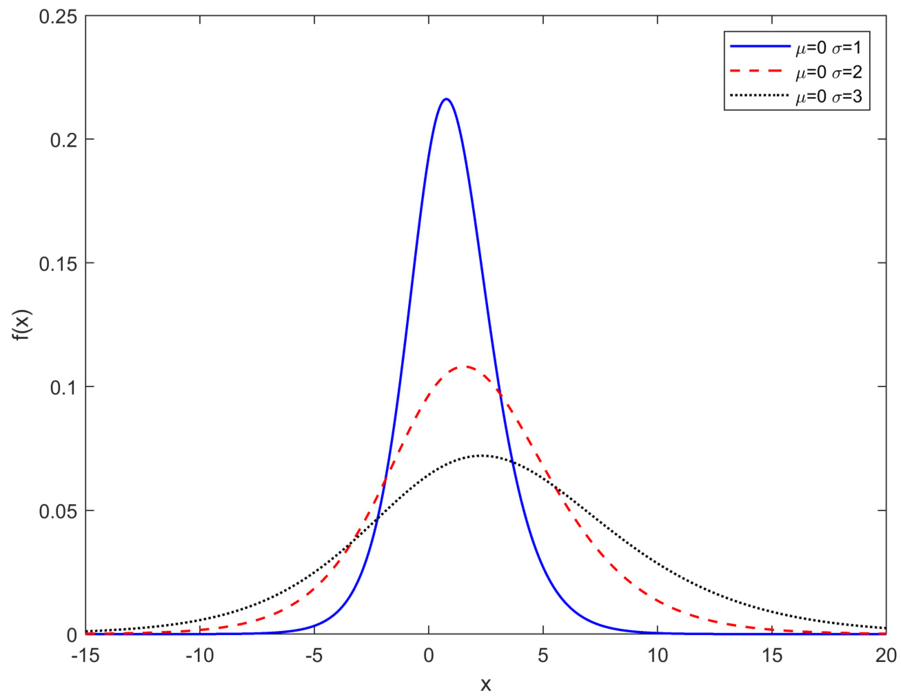
Figure 2.
Hierarchy of gray wolf population.
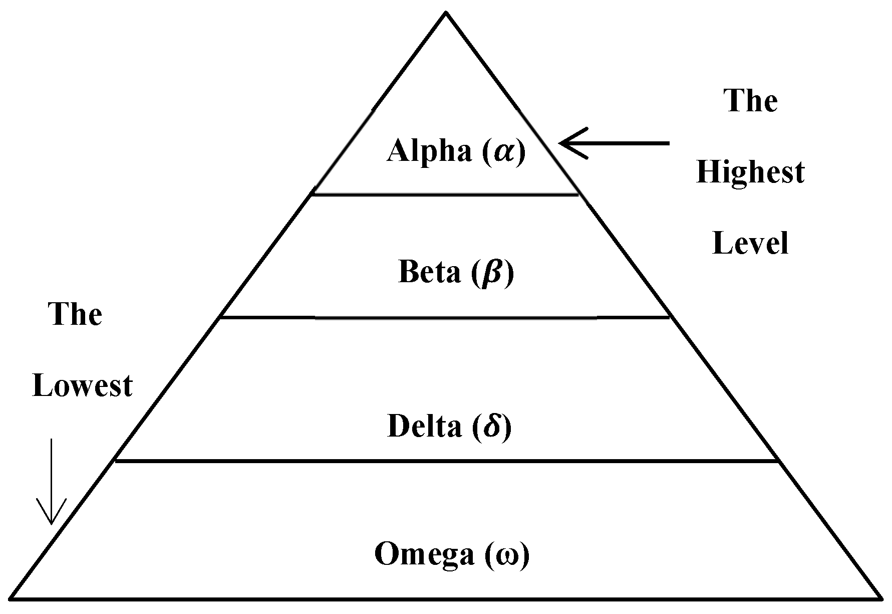
Figure 3.
Flow diagram of the GWO.
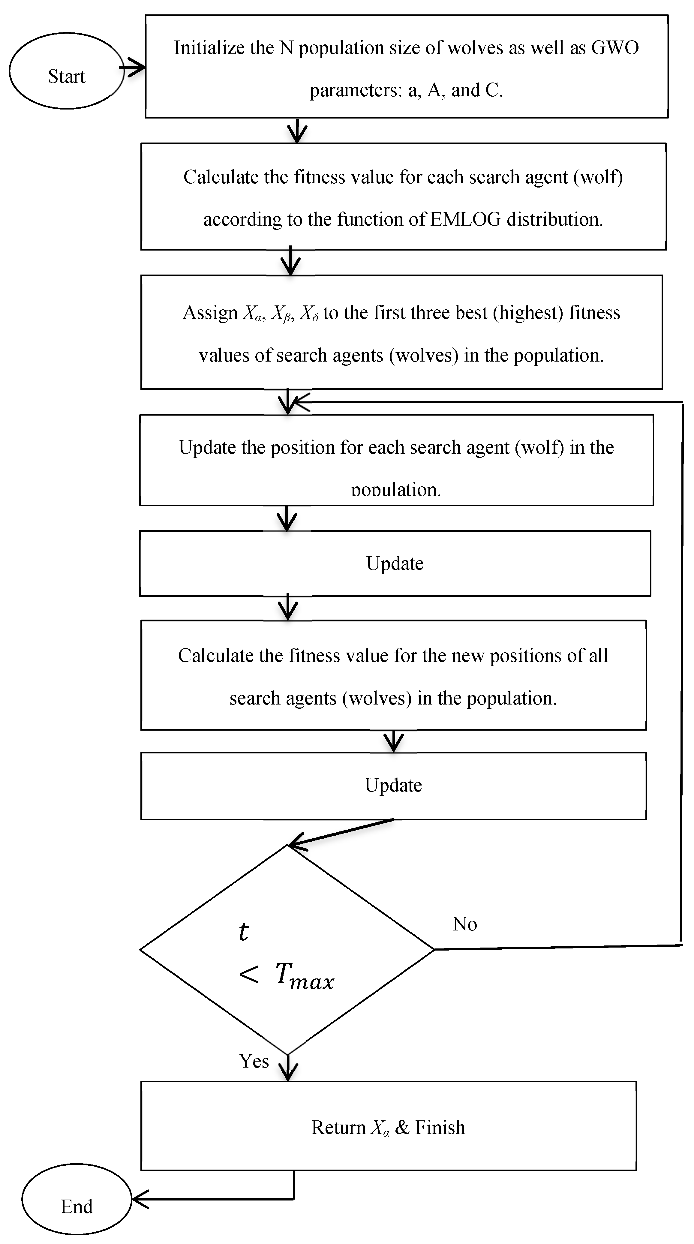

Table 1.
Simulated Mean, Bias, Variance, MSE, and Def values for the ML estimators and .
|
Method |
Mean | Variance | Bias | MSE | Mean | Variance | Bias | MSE | Def | |||||||||
| 30 | GWO | 0.0153 | 0.1463 | 0.0153 | 0.1465 | 0.9909 | 0.0219 | -0.0091 | 0.022 | 0.1685 | ||||||||
| WOA | 0.0155 | 0.1463 | 0.0155 | 0.1465 | 0.9908 | 0.0219 | -0.0092 | 0.022 | 0.1685 | |||||||||
| SCA | 0.9941 | 18.7710 | 0.9941 | 19.7592 | 0.9435 | 0.0633 | -0.0565 | 0.0665 | 19.8257 | |||||||||
| PSO | -0.0541 | 0.2880 | -0.0541 | 0.2909 | 1.0376 | 0.0820 | 0.0376 | 0.0834 | 0.3743 | |||||||||
| 50 | GWO | 0.0198 | 0.0832 | 0.0198 | 0.0836 | 0.9817 | 0.0127 | -0.0183 | 0.0130 | 0.0966 | ||||||||
| WOA | 0.0393 | 0.4822 | 0.0393 | 0.4837 | 0.9811 | 0.0133 | -0.0189 | 0.0137 | 0.4974 | |||||||||
| SCA | 0.7148 | 13.6000 | 0.7148 | 14.1109 | 0.9482 | 0.0433 | -0.0518 | 0.0460 | 14.1569 | |||||||||
| PSO | -0.0639 | 0.2861 | -0.0639 | 0.2902 | 1.0287 | 0.0762 | 0.0287 | 0.0770 | 0.3672 | |||||||||
| 100 | GWO | 0.0061 | 0.0409 | 0.0061 | 0.0409 | 0.9907 | 0.0068 | -0.0093 | 0.0069 | 0.0478 | ||||||||
| WOA | 0.0061 | 0.0409 | 0.0061 | 0.0409 | 0.9907 | 0.0068 | -0.0094 | 0.0069 | 0.0478 | |||||||||
| SCA | 0.8865 | 16.8700 | 0.8865 | 17.6559 | 0.9494 | 0.0445 | -0.0506 | 0.0471 | 17.7029 | |||||||||
| PSO | -0.0695 | 0.1923 | -0.0695 | 0.1971 | 1.0330 | 0.0615 | 0.0330 | 0.0626 | 0.2597 | |||||||||
| 150 | GWO | 0.0069 | 0.0278 | 0.0069 | 0.0278 | 0.9965 | 0.0044 | -0.0035 | 0.0044 | 0.0323 | ||||||||
| WOA | 0.0266 | 0.4275 | 0.0266 | 0.4282 | 0.9955 | 0.0054 | -0.0045 | 0.0054 | 0.4336 | |||||||||
| SCA | 0.7053 | 13.5430 | 0.7053 | 14.0404 | 0.9640 | 0.0350 | -0.0361 | 0.0363 | 14.0768 | |||||||||
| PSO | -0.0784 | 0.2568 | -0.0784 | 0.2629 | 1.0491 | 0.0815 | 0.0491 | 0.0839 | 0.3469 | |||||||||
| 200 | GWO | 0.0078 | 0.0211 | 0.0078 | 0.0212 | 0.9947 | 0.0035 | -0.0053 | 0.0035 | 0.0247 | ||||||||
| WOA | 0.0277 | 0.4208 | 0.0277 | 0.4216 | 0.9938 | 0.0043 | -0.0062 | 0.0043 | 0.4259 | |||||||||
| SCA | 0.7057 | 13.5360 | 0.7057 | 14.0340 | 0.9611 | 0.0341 | -0.0389 | 0.0356 | 14.0696 | |||||||||
| PSO | -0.0618 | 0.1450 | -0.0618 | 0.1488 | 1.0446 | 0.0656 | 0.0446 | 0.0676 | 0.2164 | |||||||||
| 30 | GWO | 0.0358 | 0.5668 | 0.0358 | 0.5681 | 1.955 | 0.0867 | -0.045 | 0.0887 | 0.6568 | ||||||||
| WOA | 0.0359 | 0.5670 | 0.0359 | 0.5683 | 1.955 | 0.0867 | -0.045 | 0.0887 | 0.6570 | |||||||||
| SCA | 0.6339 | 12.1620 | 0.6339 | 12.5638 | 1.9009 | 0.1909 | -0.0991 | 0.2007 | 12.7646 | |||||||||
| PSO | 0.0281 | 0.6443 | 0.0281 | 0.6451 | 1.9737 | 0.1036 | -0.0263 | 0.1043 | 0.7494 | |||||||||
| 50 | GWO | 0.0150 | 0.3327 | 0.0150 | 0.3329 | 1.9736 | 0.0533 | -0.0264 | 0.0540 | 0.3869 | ||||||||
| WOA | 0.0150 | 0.3327 | 0.0150 | 0.3329 | 1.9736 | 0.0533 | -0.0264 | 0.0540 | 0.3869 | |||||||||
| SCA | 0.4812 | 9.7752 | 0.4812 | 10.0068 | 1.9277 | 0.1431 | -0.0723 | 0.1483 | 10.1551 | |||||||||
| PSO | -0.0120 | 0.3795 | -0.0120 | 0.3796 | 1.9891 | 0.0623 | -0.0109 | 0.0624 | 0.4421 | |||||||||
| 100 | GWO | 0.0028 | 0.1794 | 0.0028 | 0.1794 | 1.9870 | 0.0266 | -0.0130 | 0.0268 | 0.2062 | ||||||||
| WOA | 0.0029 | 0.1795 | 0.0029 | 0.1795 | 1.9870 | 0.0266 | -0.0130 | 0.0268 | 0.2063 | |||||||||
| SCA | 0.3899 | 8.1199 | 0.3899 | 8.2719 | 1.9473 | 0.1040 | -0.0527 | 0.1068 | 8.3787 | |||||||||
| PSO | -0.0201 | 0.2167 | -0.0201 | 0.2171 | 1.9981 | 0.0343 | -0.0019 | 0.0343 | 0.2514 | |||||||||
| 150 | GWO | -0.0013 | 0.1119 | -0.0013 | 0.1119 | 1.9871 | 0.0164 | -0.0129 | 0.0166 | 0.1285 | ||||||||
| WOA | -0.0011 | 0.1120 | -0.0011 | 0.1120 | 1.9871 | 0.0164 | -0.0129 | 0.0166 | 0.1286 | |||||||||
| SCA | 0.2604 | 5.2478 | 0.2604 | 5.3156 | 1.9615 | 0.0645 | -0.0385 | 0.0660 | 5.3816 | |||||||||
| PSO | -0.0194 | 0.1379 | -0.0194 | 0.1383 | 2.0054 | 0.0344 | 0.0054 | 0.0344 | 0.1727 | |||||||||
| 200 | GWO | 0.0088 | 0.0848 | 0.0088 | 0.0849 | 1.9855 | 0.0136 | -0.0145 | 0.0138 | 0.0987 | ||||||||
| WOA | 0.0089 | 0.0848 | 0.0089 | 0.0849 | 1.9855 | 0.0136 | -0.0145 | 0.0138 | 0.0987 | |||||||||
| SCA | 0.1885 | 3.6525 | 0.1885 | 3.6880 | 1.9687 | 0.0470 | -0.0313 | 0.0480 | 3.7360 | |||||||||
| PSO | -0.0024 | 0.0988 | -0.0024 | 0.0988 | 1.9959 | 0.0238 | -0.0041 | 0.0238 | 0.1226 | |||||||||
Table 2.
Simulated Mean, Bias, Variance, MSE, and Def values for the ML estimators and .
|
Method |
Mean | Variance | Bias | MSE | Mean | Variance | Bias | MSE | Def | |||||||||||
| 30 | GWO | 1.0289 | 0.1366 | 0.0289 | 0.1374 | 0.9768 | 0.0218 | -0.0232 | 0.0223 | 0.1598 | ||||||||||
| WOA | 1.0477 | 0.4966 | 0.0477 | 0.4989 | 0.9760 | 0.0226 | -0.0240 | 0.0232 | 0.5221 | |||||||||||
| SCA | 2.0237 | 17.8320 | 1.0237 | 18.8800 | 0.9270 | 0.0652 | -0.0730 | 0.0705 | 18.9505 | |||||||||||
| PSO | 0.9325 | 0.3457 | -0.0675 | 0.3503 | 1.0387 | 0.1069 | 0.0387 | 0.1084 | 0.4587 | |||||||||||
| 50 | GWO | 1.0100 | 0.0913 | 0.0100 | 0.0914 | 1.0002 | 0.0132 | 0.0002 | 0.0132 | 0.1046 | ||||||||||
| WOA | 1.0680 | 1.1704 | 0.0680 | 1.1750 | 0.9976 | 0.0158 | -0.0024 | 0.0158 | 1.1908 | |||||||||||
| SCA | 2.2017 | 21.4220 | 1.2017 | 22.8661 | 0.9408 | 0.0688 | -0.0592 | 0.0723 | 22.9384 | |||||||||||
| PSO | 0.9635 | 0.1723 | -0.0365 | 0.1736 | 1.0285 | 0.0419 | 0.0285 | 0.0427 | 0.2163 | |||||||||||
| 100 | GWO | 1.0103 | 0.0401 | 0.0103 | 0.0402 | 0.9926 | 0.0070 | -0.0074 | 0.0071 | 0.0473 | ||||||||||
| WOA | 1.0292 | 0.4007 | 0.0292 | 0.4016 | 0.9915 | 0.0079 | -0.0085 | 0.0080 | 0.4095 | |||||||||||
| SCA | 2.0745 | 19.1190 | 1.0745 | 20.2736 | 0.9394 | 0.0546 | -0.0606 | 0.0583 | 20.3318 | |||||||||||
| PSO | 0.9286 | 0.2145 | -0.0714 | 0.2196 | 1.0408 | 0.0784 | 0.0408 | 0.0801 | 0.2997 | |||||||||||
| 150 | GWO | 1.0035 | 0.0277 | 0.0035 | 0.0277 | 0.9988 | 0.0040 | -0.0012 | 0.0040 | 0.0317 | ||||||||||
| WOA | 1.0037 | 0.0277 | 0.0037 | 0.0277 | 0.9987 | 0.0040 | -0.0013 | 0.0040 | 0.0317 | |||||||||||
| SCA | 1.7817 | 14.2310 | 0.7818 | 14.8422 | 0.9598 | 0.0400 | -0.0402 | 0.0416 | 14.8838 | |||||||||||
| PSO | 0.9331 | 0.2009 | -0.0669 | 0.2054 | 1.0434 | 0.0665 | 0.0434 | 0.0684 | 0.2738 | |||||||||||
| 200 | GWO | 1.0038 | 0.0222 | 0.0038 | 0.0222 | 0.9971 | 0.0033 | -0.0029 | 0.0033 | 0.0255 | ||||||||||
| WOA | 1.0226 | 0.3830 | 0.0226 | 0.3835 | 0.9966 | 0.0037 | -0.0034 | 0.0037 | 0.3872 | |||||||||||
| SCA | 1.8953 | 16.2030 | 0.8953 | 17.0046 | 0.9519 | 0.0445 | -0.0481 | 0.0468 | 17.0514 | |||||||||||
| PSO | 0.9356 | 0.1518 | -0.0644 | 0.1559 | 1.0407 | 0.0550 | 0.0407 | 0.0567 | 0.2126 | |||||||||||
| 30 | GWO | 1.0427 | 0.5660 | 0.0427 | 0.5678 | 1.9587 | 0.0905 | -0.0413 | 0.0922 | 0.6600 | ||||||||||
| WOA | 1.0611 | 0.9251 | 0.0611 | 0.9288 | 1.9566 | 0.0938 | -0.0434 | 0.0957 | 1.0245 | |||||||||||
| SCA | 1.7568 | 13.7140 | 0.7569 | 14.2869 | 1.8889 | 0.2220 | -0.1111 | 0.2343 | 14.5212 | |||||||||||
| PSO | 1.0185 | 0.6051 | 0.0185 | 0.6054 | 1.9751 | 0.1007 | -0.0249 | 0.1013 | 0.7068 | |||||||||||
| 50 | GWO | 1.0120 | 0.3241 | 0.0120 | 0.3242 | 1.9685 | 0.0504 | -0.0315 | 0.0514 | 0.3756 | ||||||||||
| WOA | 1.0121 | 0.3242 | 0.0121 | 0.3243 | 1.9685 | 0.0504 | -0.0315 | 0.0514 | 0.3757 | |||||||||||
| SCA | 1.4822 | 9.1786 | 0.4822 | 9.4111 | 1.9197 | 0.1437 | -0.0803 | 0.1501 | 9.5613 | |||||||||||
| PSO | 0.9932 | 0.3727 | -0.0068 | 0.3727 | 1.9882 | 0.0671 | -0.0118 | 0.0672 | 0.4400 | |||||||||||
| 100 | GWO | 0.9993 | 0.1657 | -0.0007 | 0.1657 | 1.9815 | 0.0271 | -0.0185 | 0.0274 | 0.1931 | ||||||||||
| WOA | 0.9989 | 0.1658 | -0.0011 | 0.1658 | 1.9815 | 0.0271 | -0.0185 | 0.0274 | 0.1932 | |||||||||||
| SCA | 1.3018 | 5.8544 | 0.3018 | 5.9455 | 1.9517 | 0.0862 | -0.0483 | 0.0885 | 6.0340 | |||||||||||
| PSO | 0.9628 | 0.2391 | -0.0372 | 0.2405 | 2.0028 | 0.0449 | 0.0028 | 0.0449 | 0.2854 | |||||||||||
| 150 | GWO | 1.0100 | 0.1128 | 0.0100 | 0.1129 | 1.9831 | 0.0173 | -0.0169 | 0.0176 | 0.1305 | ||||||||||
| WOA | 1.0291 | 0.4732 | 0.0291 | 0.4740 | 1.9812 | 0.0210 | -0.0188 | 0.0214 | 0.4954 | |||||||||||
| SCA | 1.1800 | 3.3322 | 0.1800 | 3.3646 | 1.9667 | 0.0506 | -0.0333 | 0.0517 | 3.4163 | |||||||||||
| PSO | 0.9913 | 0.1655 | -0.0087 | 0.1656 | 2.0034 | 0.0369 | 0.0034 | 0.0369 | 0.2025 | |||||||||||
| 200 | GWO | 1.0204 | 0.0907 | 0.0204 | 0.0911 | 1.9788 | 0.0120 | -0.0212 | 0.0124 | 0.1036 | ||||||||||
| WOA | 1.0200 | 0.0909 | 0.0200 | 0.0913 | 1.9788 | 0.0120 | -0.0212 | 0.0124 | 0.1037 | |||||||||||
| SCA | 1.2482 | 4.3658 | 0.2483 | 4.4275 | 1.9562 | 0.0565 | -0.0438 | 0.0584 | 4.4859 | |||||||||||
| PSO | 0.9955 | 0.1422 | -0.0045 | 0.1422 | 1.9972 | 0.0294 | -0.0028 | 0.0294 | 0.1716 | |||||||||||
Table 3.
Simulated Mean, Bias, Variance, MSE, and Def values for the ML estimators and .
|
Method |
Mean | Variance | Bias | MSE | Mean | Variance | Bias | MSE | Def | |||||||||||
| 30 | GWO | 2.0404 | 0.1378 | 0.0404 | 0.1394 | 0.9720 | 0.0211 | -0.0280 | 0.0219 | 0.1613 | ||||||||||
| WOA | 2.0409 | 0.1378 | 0.0409 | 0.1395 | 0.9719 | 0.0211 | -0.0281 | 0.0219 | 0.1614 | |||||||||||
| SCA | 3.3470 | 21.9970 | 1.3470 | 23.8114 | 0.9044 | 0.0802 | -0.0956 | 0.0893 | 23.9007 | |||||||||||
| PSO | 1.9795 | 0.2660 | -0.0205 | 0.2664 | 1.0245 | 0.1029 | 0.0245 | 0.1035 | 0.3699 | |||||||||||
| 50 | GWO | 2.0138 | 0.0865 | 0.0138 | 0.0867 | 0.9834 | 0.0127 | -0.0166 | 0.0130 | 0.0997 | ||||||||||
| WOA | 2.0311 | 0.4098 | 0.0311 | 0.4108 | 0.9830 | 0.0134 | -0.0171 | 0.0137 | 0.4245 | |||||||||||
| SCA | 3.3727 | 22.9320 | 1.3727 | 24.8163 | 0.9096 | 0.0756 | -0.0904 | 0.0838 | 24.9001 | |||||||||||
| PSO | 1.9425 | 0.2365 | -0.0575 | 0.2398 | 1.0414 | 0.1003 | 0.0414 | 0.1020 | 0.3418 | |||||||||||
| 100 | GWO | 2.0158 | 0.0455 | 0.0158 | 0.0457 | 0.9961 | 0.0069 | -0.0039 | 0.0069 | 0.0527 | ||||||||||
| WOA | 2.0161 | 0.0455 | 0.0161 | 0.0458 | 0.9960 | 0.0069 | -0.0040 | 0.0069 | 0.0527 | |||||||||||
| SCA | 3.1106 | 18.5920 | 1.1106 | 19.8254 | 0.9389 | 0.0594 | -0.0611 | 0.0631 | 19.8886 | |||||||||||
| PSO | 1.9336 | 0.2321 | -0.0664 | 0.2365 | 1.0511 | 0.0886 | 0.0511 | 0.0912 | 0.3277 | |||||||||||
| 150 | GWO | 1.9984 | 0.0264 | -0.0016 | 0.0264 | 0.9940 | 0.0043 | -0.0060 | 0.0043 | 0.0307 | ||||||||||
| WOA | 1.9982 | 0.0264 | -0.0018 | 0.0264 | 0.9939 | 0.0043 | -0.0061 | 0.0043 | 0.0307 | |||||||||||
| SCA | 2.8450 | 14.5540 | 0.8450 | 15.2680 | 0.9485 | 0.0451 | -0.0515 | 0.0478 | 15.3158 | |||||||||||
| PSO | 1.9311 | 0.1683 | -0.0689 | 0.1730 | 1.0391 | 0.0699 | 0.0391 | 0.0714 | 0.2445 | |||||||||||
| 200 | GWO | 2.0016 | 0.0207 | 0.0016 | 0.0207 | 1.0001 | 0.0033 | 0.0001 | 0.0033 | 0.0240 | ||||||||||
| WOA | 2.0019 | 0.0207 | 0.0019 | 0.0207 | 1.0002 | 0.0033 | 0.0002 | 0.0033 | 0.0240 | |||||||||||
| SCA | 2.7336 | 12.8290 | 0.7336 | 13.3672 | 0.9601 | 0.0408 | -0.0399 | 0.0424 | 13.4096 | |||||||||||
| PSO | 1.9299 | 0.2492 | -0.0701 | 0.2541 | 1.0501 | 0.0766 | 0.0501 | 0.0791 | 0.3332 | |||||||||||
| 30 | GWO | 2.0178 | 0.5961 | 0.0178 | 0.5964 | 1.9516 | 0.0887 | -0.0484 | 0.0910 | 0.6875 | ||||||||||
| WOA | 2.0175 | 0.5962 | 0.0175 | 0.5965 | 1.9516 | 0.0887 | -0.0484 | 0.0910 | 0.6875 | |||||||||||
| SCA | 2.6082 | 10.9120 | 0.6082 | 11.2819 | 1.8901 | 0.2033 | -0.1100 | 0.2154 | 11.4973 | |||||||||||
| PSO | 1.9918 | 0.6671 | -0.0082 | 0.6672 | 1.9734 | 0.1048 | -0.0266 | 0.1055 | 0.7727 | |||||||||||
| 50 | GWO | 1.9974 | 0.3451 | -0.0026 | 0.3451 | 1.9631 | 0.0523 | -0.0369 | 0.0537 | 0.3988 | ||||||||||
| WOA | 1.9971 | 0.3451 | -0.0029 | 0.3451 | 1.9630 | 0.0523 | -0.0370 | 0.0537 | 0.3988 | |||||||||||
| SCA | 2.5401 | 9.7643 | 0.5401 | 10.0560 | 1.9078 | 0.1589 | -0.0922 | 0.1674 | 10.2234 | |||||||||||
| PSO | 1.9639 | 0.4095 | -0.0361 | 0.4108 | 1.9886 | 0.0764 | -0.0114 | 0.0765 | 0.4873 | |||||||||||
| 100 | GWO | 2.0392 | 0.1603 | 0.0392 | 0.1618 | 1.9707 | 0.0239 | -0.0293 | 0.0248 | 0.1866 | ||||||||||
| WOA | 2.0395 | 0.1603 | 0.0395 | 0.1619 | 1.9707 | 0.0239 | -0.0293 | 0.0248 | 0.1866 | |||||||||||
| SCA | 2.1851 | 2.7227 | 0.1851 | 2.7570 | 1.9555 | 0.0534 | -0.0445 | 0.0554 | 2.8123 | |||||||||||
| PSO | 2.0046 | 0.2233 | 0.0046 | 0.2233 | 1.9917 | 0.0425 | -0.0083 | 0.0426 | 0.2659 | |||||||||||
| 150 | GWO | 1.9935 | 0.1175 | -0.0065 | 0.1175 | 1.9745 | 0.0178 | -0.0255 | 0.0185 | 0.1360 | ||||||||||
| WOA | 1.9938 | 0.1176 | -0.0062 | 0.1176 | 1.9744 | 0.0178 | -0.0256 | 0.0185 | 0.1361 | |||||||||||
| SCA | 2.0829 | 1.7308 | 0.0829 | 1.7377 | 1.9658 | 0.0364 | -0.0342 | 0.0376 | 1.7752 | |||||||||||
| PSO | 1.9712 | 0.1582 | -0.0288 | 0.1590 | 1.9931 | 0.0329 | -0.0069 | 0.0329 | 0.1920 | |||||||||||
| 200 | GWO | 1.9927 | 0.0850 | -0.0073 | 0.0851 | 1.9859 | 0.0130 | -0.0141 | 0.0132 | 0.0983 | ||||||||||
| WOA | 2.0103 | 0.4093 | 0.0103 | 0.4094 | 1.9841 | 0.0168 | -0.0159 | 0.0171 | 0.4265 | |||||||||||
| SCA | 2.1341 | 2.6630 | 0.1341 | 2.6810 | 1.9716 | 0.0429 | -0.0284 | 0.0437 | 2.7247 | |||||||||||
| PSO | 1.9731 | 0.1099 | -0.0269 | 0.1106 | 1.9989 | 0.0230 | -0.0011 | 0.0230 | 0.1336 | |||||||||||
Table 4.
Simulated Mean, Bias, Variance, MSE, and Def values for the ML estimators and .
|
Method |
Mean | Variance | Bias | MSE | Mean | Variance | Bias | MSE | Def | ||||||||||
| 30 | GWO | 3.0124 | 0.1393 | 0.0124 | 0.1395 | 0.9817 | 0.0219 | -0.0183 | 0.0222 | 0.1617 | |||||||||
| WOA | 3.0286 | 0.4277 | 0.0286 | 0.4285 | 0.9812 | 0.0227 | -0.0188 | 0.0231 | 0.4516 | ||||||||||
| SCA | 4.4228 | 22.4900 | 1.4228 | 24.5144 | 0.9025 | 0.0906 | -0.0976 | 0.1001 | 24.6145 | ||||||||||
| PSO | 2.9348 | 0.2984 | -0.0652 | 0.3027 | 1.0295 | 0.0889 | 0.0295 | 0.0898 | 0.3924 | ||||||||||
| 50 | GWO | 3.0151 | 0.0839 | 0.0151 | 0.0841 | 0.9933 | 0.0135 | -0.0067 | 0.0135 | 0.0977 | |||||||||
| WOA | 3.0146 | 0.0839 | 0.0146 | 0.0841 | 0.9931 | 0.0135 | -0.0069 | 0.0135 | 0.0977 | ||||||||||
| SCA | 4.3549 | 21.0940 | 1.3549 | 22.9298 | 0.9192 | 0.0805 | -0.0808 | 0.0870 | 23.0168 | ||||||||||
| PSO | 2.9608 | 0.2002 | -0.0392 | 0.2017 | 1.0302 | 0.0621 | 0.0302 | 0.0630 | 0.2647 | ||||||||||
| 100 | GWO | 3.0014 | 0.0441 | 0.0014 | 0.0441 | 0.9943 | 0.0064 | -0.0057 | 0.0064 | 0.0505 | |||||||||
| WOA | 3.0349 | 0.6214 | 0.0349 | 0.6226 | 0.9926 | 0.0082 | -0.0074 | 0.0083 | 0.6309 | ||||||||||
| SCA | 4.2779 | 20.1040 | 1.2779 | 21.7370 | 0.9234 | 0.0699 | -0.0767 | 0.0758 | 21.8128 | ||||||||||
| PSO | 2.9291 | 0.1967 | -0.0709 | 0.2017 | 1.0422 | 0.0639 | 0.0422 | 0.0657 | 0.2674 | ||||||||||
| 150 | GWO | 3.0066 | 0.0299 | 0.0066 | 0.0299 | 0.9987 | 0.0043 | -0.0013 | 0.0043 | 0.0342 | |||||||||
| WOA | 3.0234 | 0.3187 | 0.0234 | 0.3192 | 0.9978 | 0.0052 | -0.0022 | 0.0052 | 0.3245 | ||||||||||
| SCA | 4.1678 | 18.3840 | 1.1678 | 19.7478 | 0.9332 | 0.0639 | -0.0668 | 0.0684 | 19.8161 | ||||||||||
| PSO | 2.9208 | 0.2204 | -0.0792 | 0.2267 | 1.0512 | 0.0725 | 0.0512 | 0.0751 | 0.3018 | ||||||||||
| 200 | GWO | 3.0032 | 0.0221 | 0.0032 | 0.0221 | 0.9958 | 0.0034 | -0.0042 | 0.0034 | 0.0255 | |||||||||
| WOA | 3.0362 | 0.5993 | 0.0362 | 0.6006 | 0.9941 | 0.0051 | -0.0059 | 0.0051 | 0.6057 | ||||||||||
| SCA | 3.7839 | 12.7150 | 0.7839 | 13.3295 | 0.9521 | 0.0441 | -0.0479 | 0.0464 | 13.3759 | ||||||||||
| PSO | 2.9389 | 0.1504 | -0.0611 | 0.1541 | 1.0511 | 0.0865 | 0.0511 | 0.0891 | 0.2432 | ||||||||||
| 30 | GWO | 3.0225 | 0.6012 | 0.0225 | 0.6017 | 1.9468 | 0.0841 | -0.0532 | 0.0869 | 0.6886 | |||||||||
| WOA | 3.0224 | 0.6012 | 0.0224 | 0.6017 | 1.9468 | 0.0842 | -0.0532 | 0.0870 | 0.6887 | ||||||||||
| SCA | 3.6743 | 11.9780 | 0.6743 | 12.4327 | 1.8690 | 0.2285 | -0.1310 | 0.2457 | 12.6783 | ||||||||||
| PSO | 2.9904 | 0.6933 | -0.0096 | 0.6934 | 1.9725 | 0.1022 | -0.0275 | 0.1030 | 0.7963 | ||||||||||
| 50 | GWO | 3.0107 | 0.3429 | 0.0107 | 0.3430 | 1.9676 | 0.0537 | -0.0324 | 0.0547 | 0.3978 | |||||||||
| WOA | 3.0110 | 0.3430 | 0.0110 | 0.3431 | 1.9675 | 0.0537 | -0.0325 | 0.0548 | 0.3979 | ||||||||||
| SCA | 3.2505 | 4.3296 | 0.2505 | 4.3924 | 1.9430 | 0.1048 | -0.0570 | 0.1080 | 4.5004 | ||||||||||
| PSO | 2.9927 | 0.3700 | -0.0073 | 0.3701 | 1.9843 | 0.0655 | -0.0157 | 0.0657 | 0.4358 | ||||||||||
| 100 | GWO | 2.9949 | 0.1723 | -0.0051 | 0.1723 | 1.9730 | 0.0268 | -0.0270 | 0.0275 | 0.1999 | |||||||||
| WOA | 2.9952 | 0.1726 | -0.0048 | 0.1726 | 1.9728 | 0.0268 | -0.0272 | 0.0275 | 0.2002 | ||||||||||
| SCA | 3.2988 | 5.2872 | 0.2988 | 5.3765 | 1.9401 | 0.0927 | -0.0599 | 0.0963 | 5.4728 | ||||||||||
| PSO | 2.9636 | 0.2362 | -0.0364 | 0.2375 | 1.9934 | 0.0475 | -0.0066 | 0.0475 | 0.2851 | ||||||||||
| 150 | GWO | 2.9939 | 0.1153 | -0.0061 | 0.1153 | 1.9735 | 0.0167 | -0.0265 | 0.0174 | 0.1327 | |||||||||
| WOA | 2.9941 | 0.1153 | -0.0059 | 0.1153 | 1.9734 | 0.0167 | -0.0266 | 0.0174 | 0.1327 | ||||||||||
| SCA | 3.2557 | 4.8181 | 0.2557 | 4.8835 | 1.9407 | 0.0793 | -0.0593 | 0.0828 | 4.9663 | ||||||||||
| PSO | 2.9686 | 0.1893 | -0.0314 | 0.1903 | 1.9977 | 0.0426 | -0.0023 | 0.0426 | 0.2329 | ||||||||||
| 200 | GWO | 3.0112 | 0.0830 | 0.0112 | 0.0831 | 1.9764 | 0.0141 | -0.0236 | 0.0147 | 0.0978 | |||||||||
| WOA | 3.0112 | 0.0830 | 0.0112 | 0.0831 | 1.9764 | 0.0141 | -0.0236 | 0.0147 | 0.0978 | ||||||||||
| SCA | 3.2250 | 3.8130 | 0.2250 | 3.8636 | 1.9489 | 0.0657 | -0.0511 | 0.0683 | 3.9319 | ||||||||||
| PSO | 2.9890 | 0.1246 | -0.0110 | 0.1247 | 1.9888 | 0.0276 | -0.0112 | 0.0277 | 0.1524 | ||||||||||
Table 5.
The descriptive statistics for the tensile strength data.
| n | Min | 1st Qu. | Mean | Mode | Median | 3rd Qu. | Max | S2 | γ1 | γ2 |
| 69 | 1.3120 | 2.0892 | 2.4553 | 2.3010 | 2.4780 | 2.7797 | 3.8580 | 0.2554 | 0.1021 | 3.2253 |
Table 6.
Parameter estimates, ln L, AIC, AICc, CAIC, BIC, and HQIC values for tensile strength dataset.
Table 6.
Parameter estimates, ln L, AIC, AICc, CAIC, BIC, and HQIC values for tensile strength dataset.
| -ln L | AIC | AICC | CAIC | BIC | HQIC | ||||
| EMLOG | - | 2.2141 | 0.2472 | 50.4143 | 104.8286 | 105.0104 | 111.2968 | 109.2968 | 106.6013 |
| Gamma | 22.8047 | - | 0.1077 | 50.9856 | 105.9712 | 106.1530 | 112.4394 | 110.4394 | 107.7439 |
| Lognormal | - | 0.8762 | 0.2161 | 52.1663 | 108.3326 | 108.5144 | 114.8008 | 112.8008 | 110.1053 |
| Log-logistic | - | 0.8883 | 0.1187 | 51.4346 | 106.8692 | 107.0510 | 113.3374 | 111.3374 | 108.6419 |
| Weibull | 2.6585 | - | 5.2702 | 51.7165 | 107.4330 | 107.6148 | 113.9012 | 111.9012 | 109.2057 |
| Rayleigh | - | - | 1.7720 | 87.4975 | 176.9950 | 177.0547 | 180.2291 | 179.2291 | 177.8813 |
| Exponential | - | 2.4553 | - | 130.979 | 263.9580 | 264.0177 | 267.1921 | 266.1921 | 264.8443 |
Table 7.
The descriptive statistics for the Strengths of glass fibers data.
| n | min | 1st Qu. | mean | mode | median | 3rd Qu. | max | S2 | γ1 | γ2 |
| 63 | 0.55 | 1.3675 | 1.5068 | 1.61 | 1.59 | 1.6875 | 2.24 | 0.1051 | -0.8999 | 3.9238 |
Table 8.
Parameter estimates, ln L, AIC, AICc, CAIC, BIC, and HQIC values for Strengths of glass fibers dataset.
Table 8.
Parameter estimates, ln L, AIC, AICc, CAIC, BIC, and HQIC values for Strengths of glass fibers dataset.
| -ln L | AIC | AICC | CAIC | BIC | HQIC | ||||
| EMLOG | - | 1.3923 | 0.1550 | 18.1280 | 40.2560 | 40.4560 | 46.5423 | 44.5423 | 41.9418 |
| Gamma | 17.4396 | - | 0.0864 | 23.9515 | 51.9030 | 52.1030 | 58.1893 | 56.1893 | 53.5888 |
| Lognormal | - | 0.3811 | 0.2599 | 28.0089 | 60.0178 | 60.2178 | 66.3041 | 64.3041 | 61.7036 |
| Log-logistic | - | 0.4228 | 0.1262 | 22.7900 | 49.5800 | 49.7800 | 55.8663 | 53.8663 | 51.2658 |
| Rayleigh | - | - | 1.0895 | 49.7909 | 101.5818 | 101.6474 | 104.7249 | 103.7249 | 102.4247 |
| Exponential | - | 1.5068 | - | 88.8303 | 179.6606 | 179.7262 | 182.8037 | 181.8037 | 180.5035 |
Table 9.
The descriptive statistics for the bladder cancer patient’s data.
| n | min | 1st Qu. | mean | mode | median | 3rd Qu. | max | S2 | γ1 | γ2 |
| 128 | 0.08 | 3.3350 | 9.2094 | 2.02 | 6.28 | 11.7150 | 79.05 | 108.2132 | 3.3987 | 19.3942 |
Table 10.
Parameter estimates, ln L, AIC, AICc, CAIC, BIC, and HQIC values for the bladder cancer patient’s dataset.
Table 10.
Parameter estimates, ln L, AIC, AICc, CAIC, BIC, and HQIC values for the bladder cancer patient’s dataset.
| -ln L | AIC | AICC | CAIC | BIC | HQIC | |||
| EMLOG | 4.1273 | 3.7637 | 450.4944 | 904.9888 | 905.0848 | 912.6929 | 910.6929 | 907.3064 |
| Normal | 9.2094 | 10.4026 | 480.9070 | 965.8140 | 965.9100 | 973.5181 | 971.5181 | 968.1316 |
| Logistic | 7.4546 | 4.3693 | 453.7950 | 911.5900 | 911.6860 | 919.2941 | 917.2941 | 913.9076 |
Table 11.
The descriptive statistics for the waiting times’ data.
| n | min | 1st Qu. | mean | mode | median | 3rd Qu. | max | S2 | γ1 | γ2 |
| 100 | 0.80 | 4.65 | 9.8770 | 7.10 | 8.10 | 13.05 | 38.50 | 52.3741 | 1.4728 | 5.5403 |
Table 12.
Parameter estimates, ln L, AIC, AICc, CAIC, BIC, and HQIC values for the waiting times’ dataset.
Table 12.
Parameter estimates, ln L, AIC, AICc, CAIC, BIC, and HQIC values for the waiting times’ dataset.
| -ln L | AIC | AICC | CAIC | BIC | HQIC | |||
| EMLOG | 5.9090 | 3.2337 | 331.9065 | 667.8130 | 667.9367 | 675.0233 | 673.0233 | 669.9217 |
| Normal | 9.8770 | 7.2370 | 339.3140 | 682.6280 | 682.7517 | 689.8383 | 687.8383 | 684.7367 |
| Logistic | 8.9296 | 3.7895 | 334.6980 | 673.3960 | 673.5197 | 680.6063 | 678.6063 | 675.5047 |
Disclaimer/Publisher’s Note: The statements, opinions and data contained in all publications are solely those of the individual author(s) and contributor(s) and not of MDPI and/or the editor(s). MDPI and/or the editor(s) disclaim responsibility for any injury to people or property resulting from any ideas, methods, instructions or products referred to in the content. |
© 2024 by the authors. Licensee MDPI, Basel, Switzerland. This article is an open access article distributed under the terms and conditions of the Creative Commons Attribution (CC BY) license (http://creativecommons.org/licenses/by/4.0/).
Copyright: This open access article is published under a Creative Commons CC BY 4.0 license, which permit the free download, distribution, and reuse, provided that the author and preprint are cited in any reuse.


