Submitted:
28 October 2023
Posted:
30 October 2023
You are already at the latest version
Abstract
Water distribution networks are often susceptible to pipeline leaks caused by mechanical damages, natural hazards, corrosion, and other factors. This paper focuses on the detection of leaks in water distribution networks (WDN) using a data-driven approach based on machine learning. A hybrid Autoencoder neural network (AE) is developed, which utilizes unsupervised learning to address the issue of unbalanced data (as anomalies are rare events). The AE consists of a 3DCNN encoder, a ConvLSTM decoder, and a ConvLSTM future predictor, making the anomaly detection robust. Additionally, spatial, and temporal attention mechanisms are employed to enhance leak localization. The AE first learns the expected behavior and subsequently detects leaks by identifying deviations from this expected behavior. To evaluate the performance of the proposed method, the Water Network Tool for Resilience (WNTR) Simulator is utilized to generate water pressure and flow rate data in a water supply network. Various conditions such as fluctuating water demands, data noise, and the presence of leaks are considered using the pressure-driven demand (PDD) method. Datasets with and without pipe leaks are obtained, where the AE is trained using the dataset without leaks and tested using the dataset with simulated pipe leaks. The results, based on a benchmark WDN and a confusion matrix analysis, demonstrate that the proposed method successfully identifies leaks in 96% of cases and a false positive rate of 4% compared to a random forest model baseline based on supervised learning with a false positive rate of 15% due to unbalanced data. Furthermore, a real case study demonstrates the applicability of the developed model for leak detection in operational conditions of water supply networks using inline sensor data.
Keywords:
pipe leak detection
; machine learning
; attention mechanism
; spatio-temporal anomaly
; autoencoder
; dynamic threshold adjustment
1. Introduction
Non-revenue water loss, mostly unnoticed is a huge problem worldwide due to several factors such as underground water pipe network aging, material failure and inappropriate installation and pipe corrosion [1]. Therefore, technologies and strategies for leakage detection and location and methods for predicting water pipe failure are vital for water managers and agencies to develop countermeasures with the following significant socio-economic benefits [2]:
- Conservation of water: Water is a finite resource, and leaks in distribution networks can lead to significant water loss. Detecting and repairing leaks promptly can help conserve water and ensure its sustainable use.
- Financial savings: Water leaks can result in substantial financial losses for water utilities. By detecting leaks early, utilities can minimize the cost associated with repairing and replacing infrastructure and reduce the amount of treated water that goes to waste.
- Infrastructure integrity: Leaks in water distribution networks can indicate deteriorating infrastructure. By detecting and addressing leaks promptly, utilities can identify areas of concern and prevent further damage or potential failures.
- Environmental impact: Water leaks can have negative environmental consequences. Excessive water loss can deplete local water sources, harm ecosystems, and contribute to water scarcity in regions already facing water stress. Detecting and fixing leaks can mitigate these impacts.
- Public health and safety: Leaks in water distribution networks can lead to contamination of the water supply, posing health risks to consumers. Detecting and resolving leaks promptly helps maintain the quality and safety of drinking water.
- Operational efficiency: Effective leak detection methods can improve the operational efficiency of water utilities. By identifying and addressing leaks quickly, utilities can optimize their resources, reduce energy consumption, and enhance overall system performance.
However, pipe leak detection and localization come with various challenges such as non-uniformity of pipes, complex network topology, noise interference, limited accessibility, and cost implications.
- Non-uniformity of pipe materials and sizes: Water distribution networks consist of pipes made of various materials and sizes, making it challenging to develop universal leak detection techniques that can be applied to all pipes.
- Complex network topology: Water distribution networks often have complex network topologies with numerous interconnected pipes, valves, and fittings. This complexity poses difficulties in accurately locating leaks and identifying their sources.
- Noise interference: Background noise from traffic, construction, and other activities can interfere with leak detection methods, making it harder to detect and pinpoint leaks accurately.
- Limited accessibility: Some pipes may be buried underground or located in hard-to-reach areas, making it difficult to physically inspect them for leaks.
- Cost implications: Implementing leak detection technologies and repairing leaks can be costly, especially for large-scale water distribution networks. The challenge lies in balancing the cost of leak detection with the potential benefits of reduced water loss.
Overcoming these challenges requires the development of innovative and reliable leak detection techniques, as well as effective strategies for prioritizing and repairing leaks in a cost-effective manner.
There have been several developments in strategies which differ in complexity for leak detection and location. Basically, there exists methods based on sensors, transient signals, physical models, and data [3]. For the first method mobile optical, electromagnetic, or acoustic sensors are used. These sensors are quite expensive, their set up or their data analysis is time consuming or requires heavy human involvement (e.g., ground penetrating radar) and the quality of their measurements largely depends on the type and size of leak, materials used for the pipes and the type of the soil and soil condition where the pipeline is buried (e.g., sub bottom profiler) [4]. A method for leak detection in water distribution systems using both pressure and acoustic measurements is presented in [5]. It discusses the principles and algorithms used for leak detection and presents case studies to demonstrate the effectiveness of the approach. Furthermore, [6] proposes a modified cepstrum technique for acoustic leak detection in water distribution pipes. It discusses the algorithm and signal processing techniques used and presents experimental results to validate the effectiveness of the method.
Transient signal of pressure or sound can be used to detect and localize leaks [7,8]. For example, in [9] and in [10], a transient-based method for leak detection in water distribution pipes is presented. It discusses the principles and algorithms used, as well as the experimental setup and results to demonstrate the effectiveness of the approach. [11, 12] gives a review paper which provides an overview of leak detection methods in water distribution networks using transients. It discusses the principles, advantages, and limitations of transient-based techniques, as well as the challenges and future research directions in this field. Further, [13] proposes a wavelet analysis-based method for leak detection in water distribution pipes using transient signals. It discusses the algorithm and signal processing techniques used, as well as the experimental results to demonstrate the effectiveness of the approach. [14] presents a method for leak detection in water distribution pipes using the Hilbert-Huang transform applied to transient signals. It discusses the algorithm and signal processing techniques used, as well as the experimental results to validate the effectiveness of the approach. Unfortunately, transient signals decay with distance which means they should be of very high spatial and temporal resolution to be used appropriately [15]. Like the transient signal approach is the Negative Pressure Wave (NPW) technique [16]. It is the most popular and cost-effective technique. Pressure analysis of several transducers makes it possible to both identify and locate the leak. However, there are several challenges to analyzing such pressure transducer data. It is extremely noisy (low quality data), there is a high noise to data ratio, requiring computationally expensive processes to denoise and make legible. Secondly, the initial pressure drop caused by the leak will dissipate quickly and the negative pressure wave decays as the system reaches a new equilibrium condition. The pressure data is also convoluted with both known and spontaneous events (i.e., multiple pumps and possible leak events).
Strategies based on physical models of the WDN e.g., EPANET are frequently used, and they can identify leaks and localize their positions [17,18] They are based on mathematical models to analyze system behavior and identify anomalies that may indicate the presence of leaks. These methods utilize hydraulic and/or statistical models to simulate the flow and pressure conditions in the network and compare them with measured data to detect deviations that could be caused by leaks. However, these methods also have limitations, such as the need for accurate network models and calibration, the reliance on accurate input data, and the computational complexity of some modeling approaches. As with all physical models in all domains, detailed information which is difficult to find such as the user demand, pipe condition, water pressure distribution, etc. is required for a hydraulic model to be implemented. Furthermore, soft sensing approaches using hydraulic modeling are vulnerable to measurement uncertainties, noise, and calibration drifts. This makes physical model-based system very difficult to implement in real systems [18]. Therefore, there is a clear need for fast models that can tolerate uncertainties and noisy data while minimizing detection time and false-positive and false-negative alarms.
Emerging are expert knowledge [19] and data-based methods. Usually, these methods require only input output data which is readily available from data acquisition (SCADA) systems, real-time monitoring data of water pressure and/or flow rate in comparison to the comprehensive data required by the physical-based models. Data driven methods based on machine learning have been studied for example in [20]. Primary challenges of using data driven methods have been described in [21]. They include problem with unbalanced data when using supervised learning and fluctuating water use patterns [22]. Some authors have attempted to solve these issues e.g., [21] and [23] using prediction-classification methods or as in [24] by using adaptive methods for predicting water demand at night when water use is low. However, these methods require that the water demand trend is predictable to avoid false alarms. Furthermore, water pressure can be affected similarly be a highwater demand or by a leak. These influences can be very difficult to differentiate when considering only single nodes for training without considering spatial relationships. For example, an intact water pipeline at high average water demand ratio can show similar behavior as a leaking pipe with low average water demand ratio. Machine Learning model, however, allows to extract features from the spatial pattern in the pressure data at multiple nodes and therefore allows to differentiate leaking versus non-leaking conditions as shown by [21] with his DenseNet neural network that the spatial relationship between multiple nodes in the water distribution network can be used to mitigate these false alarms. Unfortunately, the authors used spatial information in supervised learning which face the previously mentioned problem of unbalanced data due to insufficient amount of data under leaking conditions.
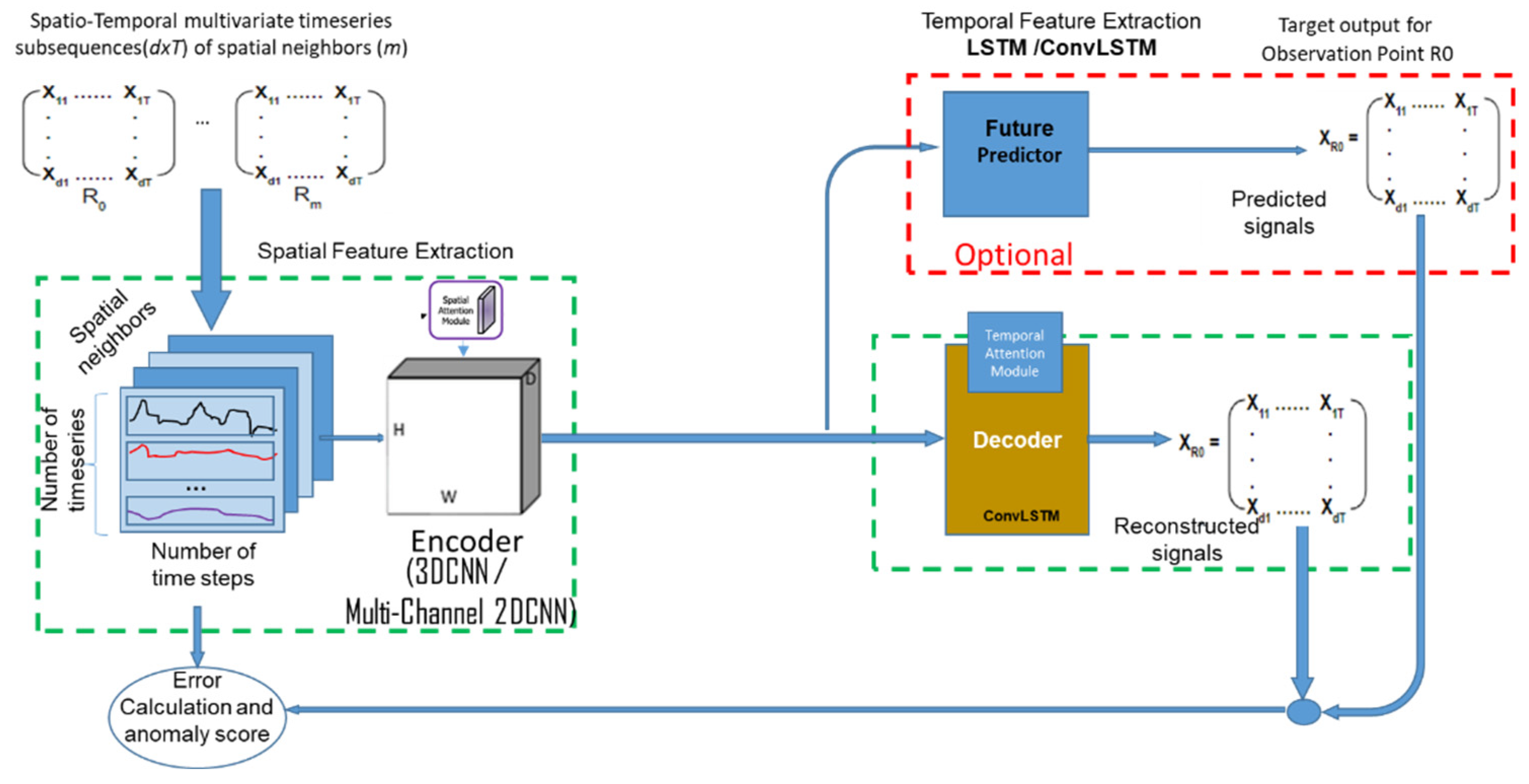
In this paper we developed hybrid deep learning framework encoder-decoder Neural Network for leak detection and localization using data generated by a pressure driven demand hydraulic simulator based on EPANET and WNTR. The model treats the pipe leaks as anomalies. The hybrid autoencoder network is composed of a 3D convolutional neural network (CNN) based spatio-temporal encoder and a convolutional Long Short-Term Memory (ConvLSTM) network-based spatio-temporal decoder as well as future predictor. A spatial attention mechanism is used to improve the pipe leak localization and interpretability of the results. The complete model is designed to be trained in a truly unsupervised fashion for anomaly detection in non-image spatio-temporal datasets.
As in all anomaly detection methods based on unsupervised learning, it first learns the expected behavior and detect leaks by deviations from the expected behavior. To overcome the challenges of unbalanced data and uncertainty of user demand described previously this novel method based on Autoencoder for leak detection uses both the spatial and temporal information and requires training data from the normal behavior only. The spatial pattern among a group of nodes is used in leak detection and identify leak conditions. The combination of reconstruction and future prediction makes the system robust for anomaly detection.
The demonstration of our method for pipe leak detection is done through a benchmark study and a real case study. These demonstrations help to evaluate the performance and effectiveness of the method in detecting leaks in water distribution networks.
2. Materials and Methods
2.1. Study water distribution networks
Two water distribution networks were used for the studies in this paper. The first water distribution network for this study is shown in Figure 1. The D-Town network, which was studied by [25], is made up of 399 points, 443 pipes, 7 tanks, 5 valves, and 11 pumps that are divided into 5 pumping stations. This information is illustrated in Figure 2. In accordance with Item 2, all nodes in the network were calibrated to have the same emission coefficient, Ce, which was set to 0.03. This resulted in a water loss of 28%. The initial daily water consumption in the network is 159,617 cubic meters, which, based on an average consumption of 150 liters per person per day, corresponds to a population of 1.06 million people.
This network was utilized to evaluate the proposed method for leak detection and classification. To assess the performance of the method, two common evaluation metrics were employed: the confusion matrix and the ROC curve. The confusion matrix is a tabular representation that summarizes the results of a classification model. It provides a detailed breakdown of the number of true positives (TP), true negatives (TN), false positives (FP), and false negatives (FN) predicted by the model. In the context of leak detection, true positives represent correctly identified leaks, true negatives indicate correctly identified non-leak instances, false positives represent instances where non-leaks were incorrectly classified as leaks, and false negatives indicate instances where leaks were missed or not detected. By analyzing the confusion matrix, it is possible to assess the accuracy and performance of the proposed method. The values in the matrix can be used to calculate various evaluation metrics, such as precision, recall, and F1-score, which provide insights into the model’s ability to correctly classify leaks and non-leaks. In addition to the confusion matrix, the Receiver Operating Characteristic (ROC) curve is another commonly used evaluation tool for classification models. The ROC curve plots the true positive rate (sensitivity) against the false positive rate (1-specificity) at different classification thresholds. It visualizes the trade-off between correctly identifying leaks and incorrectly classifying non-leaks as leaks. The area under the ROC curve (AUC) is a metric that quantifies the overall performance of the classification model. A higher AUC indicates a better ability to distinguish between leaks and non-leaks, with values closer to 1 indicating higher accuracy. By utilizing both the confusion matrix and the ROC curve, the study was able to comprehensively evaluate the performance of the proposed method for leak detection and classification in the D-Town water distribution network. These evaluation metrics provide valuable insights into the accuracy, precision, and overall effectiveness of the method in identifying and classifying leaks in the network.
The second case study presented focuses on a real water distribution network (WDN). This network consists of 112 nodes and 126 connection pipelines, with water being supplied by a single reservoir. The elevations of the nodes in the network range from 90 m to 120 m, indicating variations in the terrain. Additionally, the length of the pipes in the network ranges from 90 m to 130 m, suggesting different distances and levels of connectivity between the nodes. The purpose of using this real WDN in the study was to evaluate the practicability and applicability of the proposed model in real-world situations. By utilizing a real network, the study aimed to assess the model’s performance and effectiveness in a realistic setting, where variations in elevations, pipe lengths, and network topology are present. The evaluation of the model in this real WDN involved the application of the proposed method for leak detection and classification. The model was tested on this network to detect and classify leaks accurately, and its performance was evaluated using evaluation metrics such as the confusion matrix. By conducting the evaluation on a real WDN, the study aimed to provide practical insights into the model’s performance and its potential for real-world implementation. The results obtained from this case study would help validate the effectiveness of the model and provide valuable information for decision-makers and practitioners in the field of water distribution network management.
3. Methods
The approach is shown in Figure 1 and is composed of three stages. It starts with the generation of data for the normal case and for cases with pipeline leakages using a hydraulic model for water distribution networks. In this pre-processing stage multivariate spatio-temporal dataset is generated so that the deep autoencoder network can exploit the spatial and temporal contexts jointly. The subsequent stage is the data reconstruction and prediction stage, which is executed by a deep hybrid autoencoder network. The Autoencoder Neural Network is trained to learn the normal situation using the dataset for the normal case. The third stage is the anomaly detection stage, which is performed based on the reconstruction error. After training the Autoencoder Neural Network can be used to find anomalies (pipeline leaks) in the test dataset. Hereby, a threshold is given on the deviations of the signals from the normal case and violation of the threshold is an indication of an anomaly. These subcomponents will be described in the following sections starting with data generation.
3.1. Data generation
We want to account for fluctuation in water demand, data noise, and leaking so called off-design conditions. Therefore, for the data generation a hydraulic model for a water distribution system capable of accounting for pressure-driven (also known as head-driven) demand and leakage flow at pipe level is required. There are several hydraulic models which have been developed to incorporate pressure-driven demand analysis (e.g., in; [26] and [27]). The primary goal of the standard EPANET (strict demand-driven approach) implementation is to simulate operated networks correctly. In such a model the water demands are assumed as defined inputs. A node is described by water and energy mass balance equations. The water balance equation 1 prescribes that under no leak condition the inflow of water to a pipe node must be equal to the outflow of water.
where denites the set of pipes connected to the node , is the flow rate of water into node through pipe p (m3/s), is the actual water demand at node (m3/s), and is the number of nodes in the water distribution network.
The energy balances the total water head resulting from the kinetic energy, hydraulic potential energy, and gravitational potential energy (elevation head). For this equation we refer to [28].
However, when simulating systems with fluctuation in water demand, data noise, and pipeline leakages, reduced pressures are quite common and requires a hydraulic model with PDD consideration [26]. The values of nodes in a PDD hydraulic model depends on the current local pressure as given in Equation 2. The model assumes that each node is in one of three states: Fully served: the node can withdraw its nominal demand. Partially served: the node withdraws a reduced demand or non-served: if P = 0, the node is unable to withdraw any water.
Water Network Tool for Resilience (WNTR) is a python package based on EPANET where the off-design hydraulic network is implemented and is used to build the water supply network and solve the hydraulic equations [27]. For data collection, the package was adopted to run iteratively with different combinations of random parameters that describes the water supply network in design and off-design form by changing water demand in each range, adding noise to data, and adding leaks to the water distribution network. Leaks are modelled by the orifice equation 2 [27].
This custom demand described in Equation 2 rapidly increases to a randomized total demand. Such leak demands were placed at random locations and times. The leaks can be either randomly generated or fixed at predefined times and locations. The number and magnitude of leaks can also vary, creating more complex situations. The area values will be chosen randomly between 0.00012m² and 0.00050m², values used in [29]
The ranges for the randomness of water usage, pipe conditions and data noise were taken from literature. According to [30] baseline water demand can fluctuate 0.3 times to 1.3 times depending on the time of the day. The pipe conditions are described with the dimensionless roughness coefficient with values which are uniformly distributed between 100 to 300. Gaussian noise N(0, σ) is added to the water distribution network to account for the uncertainty in the data in general. For the case study, the baseline demand of each service node is taken from the range of 0.008 to 0.012 L/s assuming a Gaussian distribution with variance σ = 0.01L/s. Eleven demand ratios from 0.3 to 1.3 are considered during the data generation with the hydraulic model for the WSN. The lower and the upper bounds of the pressure head at the nodes are set to 5 m and 30 m, respectively. Several simulations were conducted for each combination of parameters while recording the water pressure at all nodes. For the test dataset similar simulations were run, but this time some pipelines were cutoff, and data recorded.
The WNTR simulator need some improvement to avoid memory leaks. The problem is that the simulator saves all intermediate and output data to the RAM that can easily cause memory overflow. To avoid this, the input data is sliced into segments saving only the final outputs to the memory. Finally, these outputs were rescaled back to the original timescale.
For modelling the individual water networks’ nodes, the nearest neighbor search is applied to each target node to find its nearest neighbors within a given distance which enables using a limited set of sensors. The distance between nodes is calculated by Dijkstra path finding algorithm which find closest sensors weighted by their connection length. Using the WNTR simulator the pressures of the closest nodes are taken as inputs and the target nodes as output. With this data two modelling approaches can be followed, 1) A model can be created for each target node, or the data of all nodes can be concatenated into a 3D tensor to model all the nodes with one model. The 3D tensor in Figure 2 is built using multivariate time series data from different spatial sensors , where i=1. . . m are the nearest neighbors. The sliding window technique of window size is used to build the 3-dimensional data. represents the number of univariate timeseries. The best m can be found empirically for each problem domain.
3.2. Deep learning autoencoder
The proposed autoencoder network comprises a 3D convolutional neural network (CNN), and a spatio-temporal decoder component which has a Convolutional Long Short-term Memory (ConvLSTM) network and spatial and temporal attention mechanism. Its structure is shown in Figure 3. The encoder part is based on a 3D CNN, which can capture spatial and temporal features from the input data. It takes in a sequence of 3D volumetric data, which represents the water system condition over time, and extracts relevant features using the convolutional layers. These layers perform convolutions in both the spatial and temporal dimensions, allowing the network to learn spatial and temporal patterns in the data. To effectively use the information related to location and time in the input, we have made modifications to the 3DCNN model by incorporating an attention mechanism. This involves assigning dynamic weights to the input features based on their spatial importance. By utilizing the spatial attention module and temporal attention module, we can dynamically adjust the attention weights, thereby improving the performance of the model.
The decoder part of the network is a Convolutional Long Short-term Memory (ConvLSTM) network. ConvLSTM is an extension of the traditional LSTM architecture that can handle spatio-temporal data. It was introduced by [31] for abnormal event detection and motion estimation in videos, because of its capability to utilize both spatial and temporal information. It uses convolutional operations instead of fully connected layers to process both spatial and temporal information. The ConvLSTM network takes the encoded features from the 3D CNN and decodes them to reconstruct the input data.
By combining the 3D CNN and ConvLSTM network, the autoencoder can effectively capture both spatial and temporal dependencies in the input data. This hybrid approach allows for accurate detection of pipe leaks by learning and reconstructing the normal condition of the pipe. Any deviations from the normal condition can be identified as potential leaks.
[32] and [33] have shown that combining anomaly detection architectures based on the combination of reconstruction and future prediction make anomaly detection system robust against noise. Reconstruction methods in autoencoders aim to minimize the reconstruction error for training data, which means they try to reconstruct the input data as accurately as possible. However, this approach may not guarantee large reconstruction errors for abnormal events. Abnormal events may still be reconstructed with relatively low error if they share some similarities with the normal training data. On the other hand, future prediction methods take a different approach. They operate under the assumption that normal events are predictable, meaning that the future instances can be accurately predicted based on the past data. In contrast, abnormal events are considered unpredictable, and their future instances cannot be accurately predicted based on the past data. Therefore, in this paper an approach that combines the methods is developed to conduct forecasting and reconstruction sequentially. Forecasting makes the reconstruction errors large enough to facilitate the identification of abnormal events, while reconstruction helps enhance the predicted future from normal events. Specifically, two ConvLSTM network blocks are connected to the decoder part. One block works in the form of forecaster, and the other reconstructs the signals. By focusing on the predictability of future data, this approach can effectively identify abnormal events that are not captured by reconstruction methods.
Overall, the proposed autoencoder network for pipe leak detection combines the strengths of 3D CNN and ConvLSTM to effectively capture and process spatial and temporal information, enabling accurate detection of pipe leaks. Based on 3D convolutional operations on the multivariate spatio-temporal data, the temporal features along with the spatial features can be better preserved. The input data are reconstructed as a 3-dimensional cuboid by stacking multivariate data frames. By applying such an idea, dimensionality reduction both in spatial and temporal context can be achieved for a given input window during the encoding phase.
For each target node a sample dataset with water pressure information of its neighborhood generated as previously described is used for training. 70% of the normal non-leaking dataset is normalized and used for training. The rest 30% of the normal non-leaking dataset is used for validation. For testing the model, the dataset from the leaking conditions is used but normalized based on the mean and variance values of non-leaking dataset. Hereby two scenarios were simulated, 1) leak in the target node and 2 leaks in the input pipelines (i.e., leaks in the neighbors).
Figure 3.
Structure of the hybrid autoencoder for leak detection.
3.3. Anomaly detection stage (Leak detection)
In this stage the anomalies (leaks) are found by calculating the sum of the reconstruction and forecasting errors as anomaly score. For a model trained by dataset of only non-leak condition, a large reconstruction error occurs if data of leaking condition are supplied at the input, because the relationship described by the trained AE neural network is not valid under such condition. By setting a threshold in the construction error, the AE model can classify if a set of data corresponds to a leaking situation or a non-leaking situation.
Let and be univariate time series data representing one of the reconstructed features and its forecasts and T and H are the length of the input and prediction windows, respectively. Each data point represents a data reading for that feature at time instance . The mean absolute error (MAE) is used to calculate the reconstruction and forecast error for the given period (input window +prediction window) for each feature as
where is the observed value and is the reconstructed value at time instance .
Dynamic threshold adjustment based on the moving averages is used to continuously update the threshold based on the latest observations.
3.4. Evaluation
The anomaly score in the proposed method is calculated based on two factors: the difference in gradient between the model (for early detection) and the real values, and the mean absolute error. The difference in gradient measures the deviation between the predicted values from the model and the actual values in the water distribution network. A larger difference indicates a higher likelihood of an anomaly or abnormal behavior in the system. The mean absolute error, on the other hand, quantifies the average magnitude of the errors between the predicted and actual values. A higher mean absolute error suggests a higher level of uncertainty or inaccuracy in the model’s predictions. By combining these two factors, the anomaly score provides a comprehensive assessment of the deviation and uncertainty in the system. A higher anomaly score indicates a higher probability of an anomaly or abnormal event occurring in the water distribution network. For anomaly detection the value of the threshold of the reconstruction and forecast errors for deciding whether values are anomalies need to be determined. Therefore, a statistics histogram of reconstruction and forecast errors in non-leaking and leaking conditions was constructed for the case study to see whether the two conditions are separable. For localization of the pipe leaks, the individual errors of the individual features are examined to find the feature with the maximum contribution to Equation 4. Further spatial attention weights generated by the attention mechanism. are analyzed to find the relationships between the nodes. These weights indicate the importance or relevance of different regions or pipes in the network for leak localization. The attention weights are visualized to gain insights into the network’s behavior. This is done by overlaying the attention weights on a map of the water distribution network and highlighting the pipes with high attention weights. These areas are likely to have leaks or require further investigation.
As the target nodes take their neighbors’ information as inputs, the presence of large errors in the target node can result from themselves having leaks or their neighbors. Once a target node is identified as anomalous or abnormal, additional investigation is conducted by examining its neighboring nodes. The purpose of this investigation is to determine the exact cause or source of the anomaly. By analyzing the information received from the neighbors, researchers aim to identify whether the target node itself is responsible for the error or if it is caused by the information received from its neighbors.
This approach allows for the detection of leaks and other anomalies in the system by identifying instances where the anomaly score exceeds a certain threshold. By monitoring the anomaly score over time, it is possible to detect and respond to anomalies promptly, minimizing the impact on the network and improving its overall performance.
4. Results
This The hydraulic model of the D-Town WSN is built using the WNTR software. The model considers the actual water demands at each node and simulates both non-leaking and leaking scenarios to generate the necessary data sets for evaluating the leak detection algorithm. The results are as follows: The histogram of the reconstruction errors of the non-leaking and leaking conditions is shown in Figure 4. the reconstruction error of data under normal non-leaking situation is small, with 97.5% of reconstruction error less than 1.5e-3. The validation of the dataset under leaking condition shows large reconstruction errors. Fortunately, this clear difference in behavior makes the selection of the threshold values much easier. The difference can be used to define the threshold for leak detection Figure 4 shows that for the case study, a threshold of reconstruction error of 4e-3 can be used to differentiate the leak versus non-leak situations.
For evaluating the network under leak conditions, the network has been subjected to various leak scenarios in a period of one week, each with different characteristics. Some leaks showed a gradual increase in flow over time, while others had a sudden and immediate appearance. Figure 5 provides a visual representation of the flow behavior for each node where leaks were simulated.
The data indicates that the leaks were not clustered together but rather occurred at spaced intervals. However, there was also a situation where leaks happened simultaneously in different locations, specifically at nodes J372 and J1025. Overall, this information highlights the complexity and diversity of the leak scenarios that were simulated on the network.
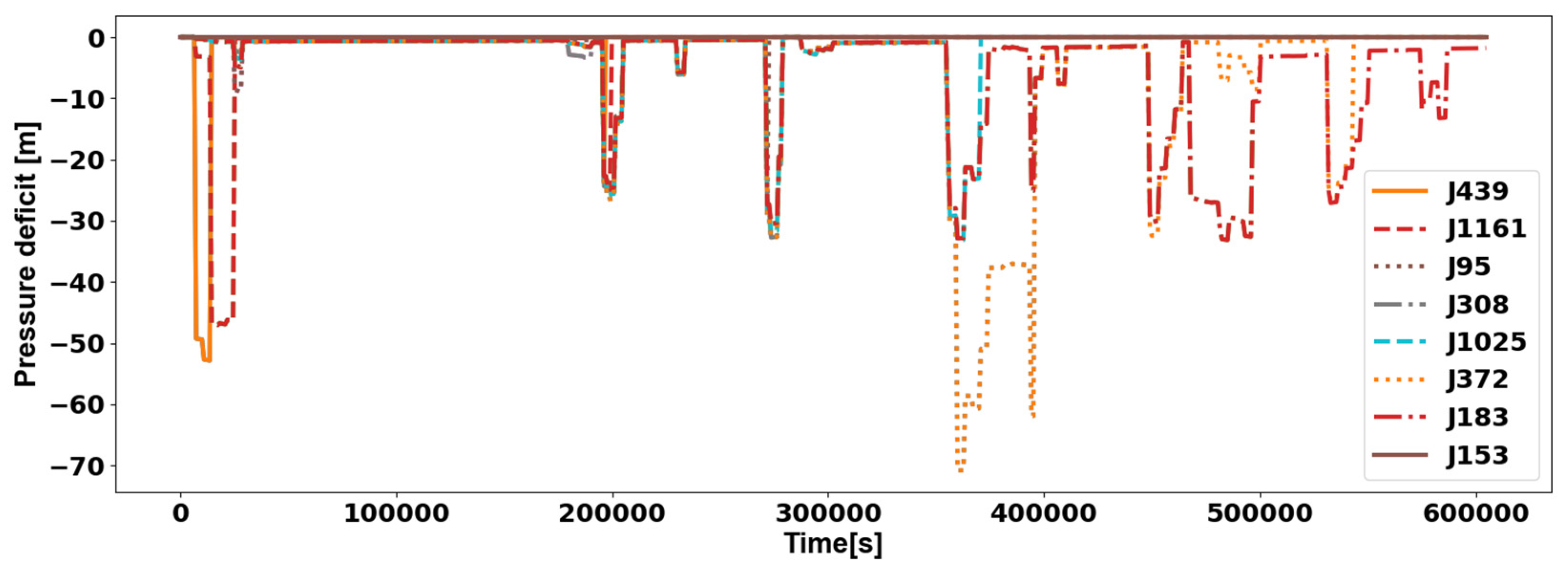
Figure 6 provide valuable information about the behavior of the water distribution system during both normal operation and leak events and shows the values of the pressure deficit throughout the simulation over time. The pressure deficit is an important parameter to monitor as it indicates the difference between the actual pressure in the network and the desired pressure. In a well-functioning system, the pressure deficit should be minimal and within acceptable limits. However, during leak events, the pressure deficit increases significantly, indicating a drop in pressure. By examining Figure 5, it is possible to identify the moments when there are leaks in the system. These are indicated by high pressure deficits, which correspond to a sudden drop in pressure. This information is crucial for leak detection, as it allows for the timely identification of leaks and the implementation of appropriate measures for repair and maintenance and allows for the evaluation of the effectiveness of the leak detection method.
Overall, the analysis of Figure 6 demonstrates the importance of monitoring pressure deficit and other system parameters to detect and evaluate the impact of leaks. The visualization provided by these plots allows for a better understanding of the behavior of the system during normal operation and leak events, enabling effective leak detection and management.
Figure 6.
Pressure deficit in selected nodes of the water distributions system in leakage conditions.
Figure 6.
Pressure deficit in selected nodes of the water distributions system in leakage conditions.
The discussion continues with the analysis of Figure 7a, which demonstrates that the proposed method successfully detects all the leaks in the network and accurately predicts their duration. This is a crucial aspect of leak detection as it allows for timely repairs and maintenance to be carried out. Figure 7b provides further insight into the causes of the detected leaks, showing that they correspond to the registered causes. This indicates that the method can accurately identify the sources of the leaks, which is essential for effective leak management and mitigation.
To provide a comprehensive evaluation of the method’s performance, an unbalanced dataset of size 6375 is used as input, out of which only 13% (834) specifically pertain to leakage signals. Hereby, a data ratio of 60/20/20 is used in the training, validation, and test of the model. The resulting confusion matrix of our method is presented in Table 1. This matrix summarizes the results and allows for a better understanding of the classification accuracy. It shows the number of true positives, true negatives, false positives, and false negatives, providing a quantitative assessment of the method’s performance. With this unbalanced data, our method shows a true false rate of only 4% compared to the random forest model showing 15% false positives and 0.01% false negatives. The random forest method based on supervised shows as expected that it ignores fewer classes.
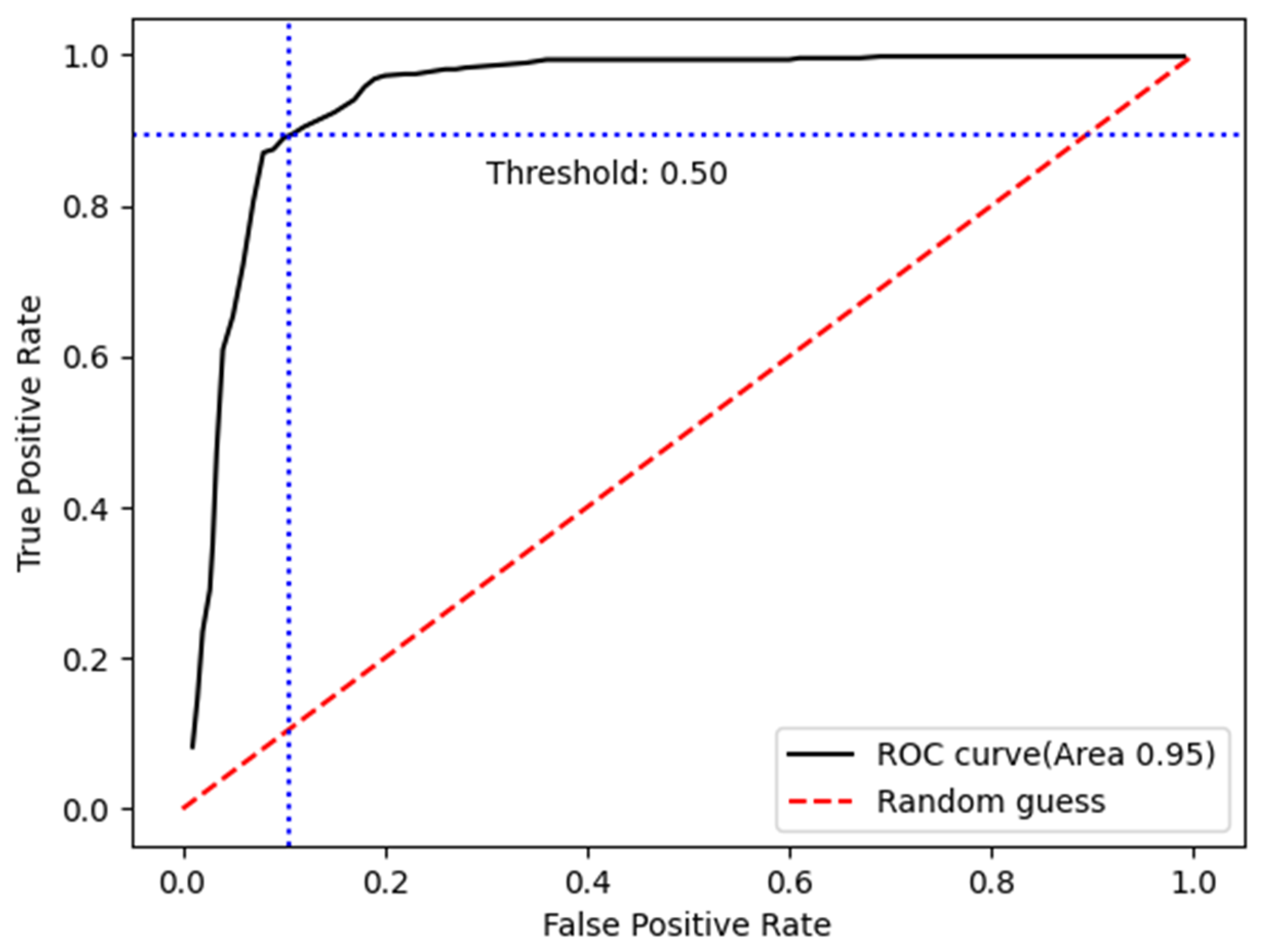
Additionally, the Receiver Operating Characteristic (ROC) curve in Figure 8 illustrates the trade-off between the true positive rate (sensitivity) and the false positive rate (1-specificity) at different classification thresholds. The ROC curve is a common tool used to evaluate the performance of classification models. A higher area under the curve (AUC) indicates a better performance of the method in distinguishing between positive and negative instances.
Overall, the analysis of Figure 7a, Figure 7b, Table 1, and Figure 8 demonstrates that the proposed method is effective in detecting and classifying leaks in the water distribution network. It accurately identifies the leaks, predicts their duration, and provides insights into their causes. This information can be used to prioritize repairs, allocate resources efficiently, and ultimately reduce water loss in the network.
Figure 7.
a) Identified leaks and their duration, b) cause of anomalies.
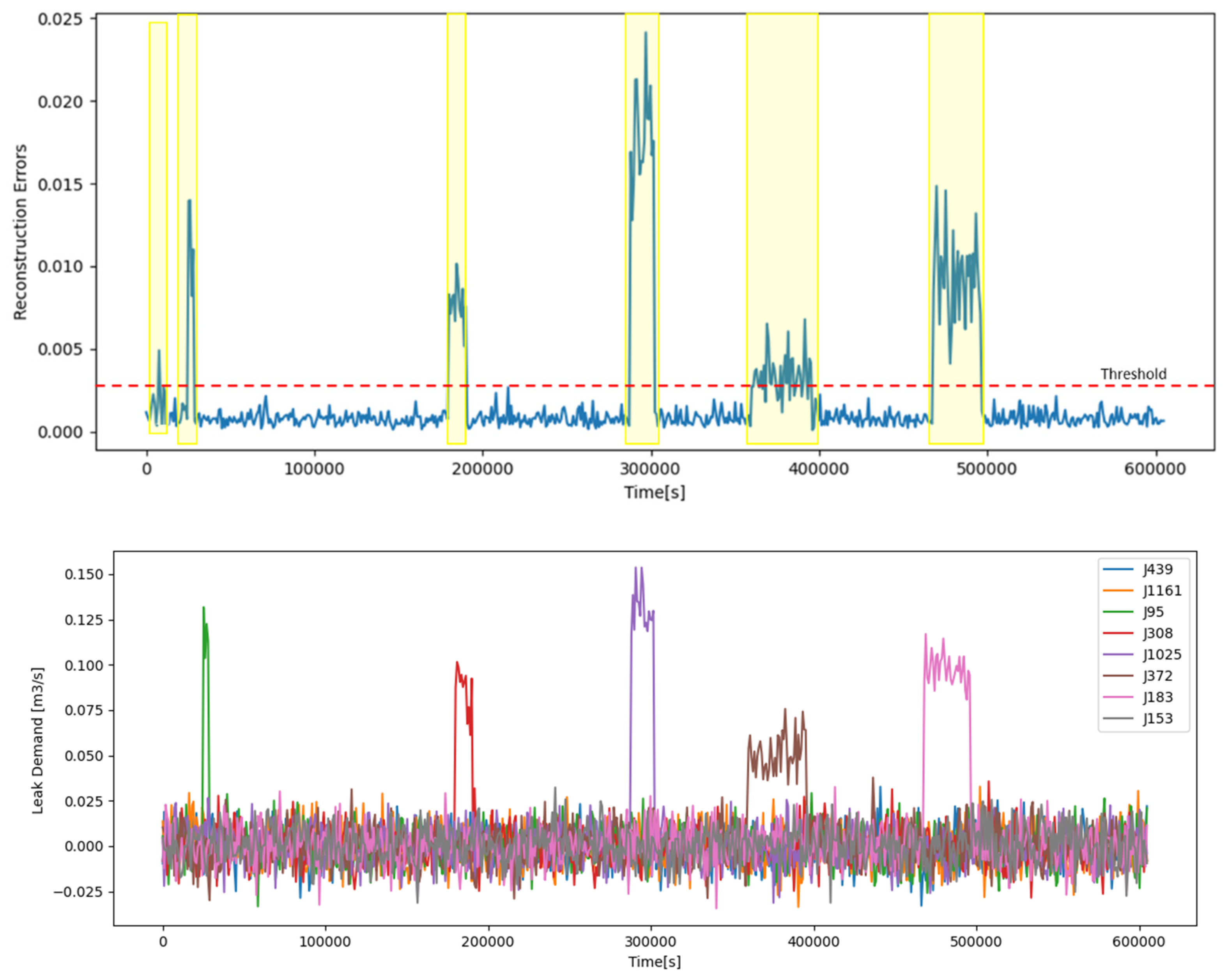

Table 1.
Confusion matrix.
| Non leakage prediction | Leakage prediction | |||
|---|---|---|---|---|
| Our method | Random forest | Our method | Random forest | |
| Non leakage reality | 1063(0.96) | 930(84) | 45(0.04) | 191(0.15) |
| Leakage reality | 0.0 | 19(0,01) | 166(1.0) | 134(0.81) |
Figure 8.
ROC an AUC of the pipe leak detection based on the benchmark water distribution network.
The evaluation of the confusion matrix in terms of accuracy reveals that the detection method achieved an 86% score. According to reference [34], this indicates a high level of accuracy in leak detection. This suggests that the proposed leak detection process in this research ensures a reliable detection rate using existing monitoring data. The methodology proposed is straightforward and efficient, demonstrating its effectiveness in leak detection.
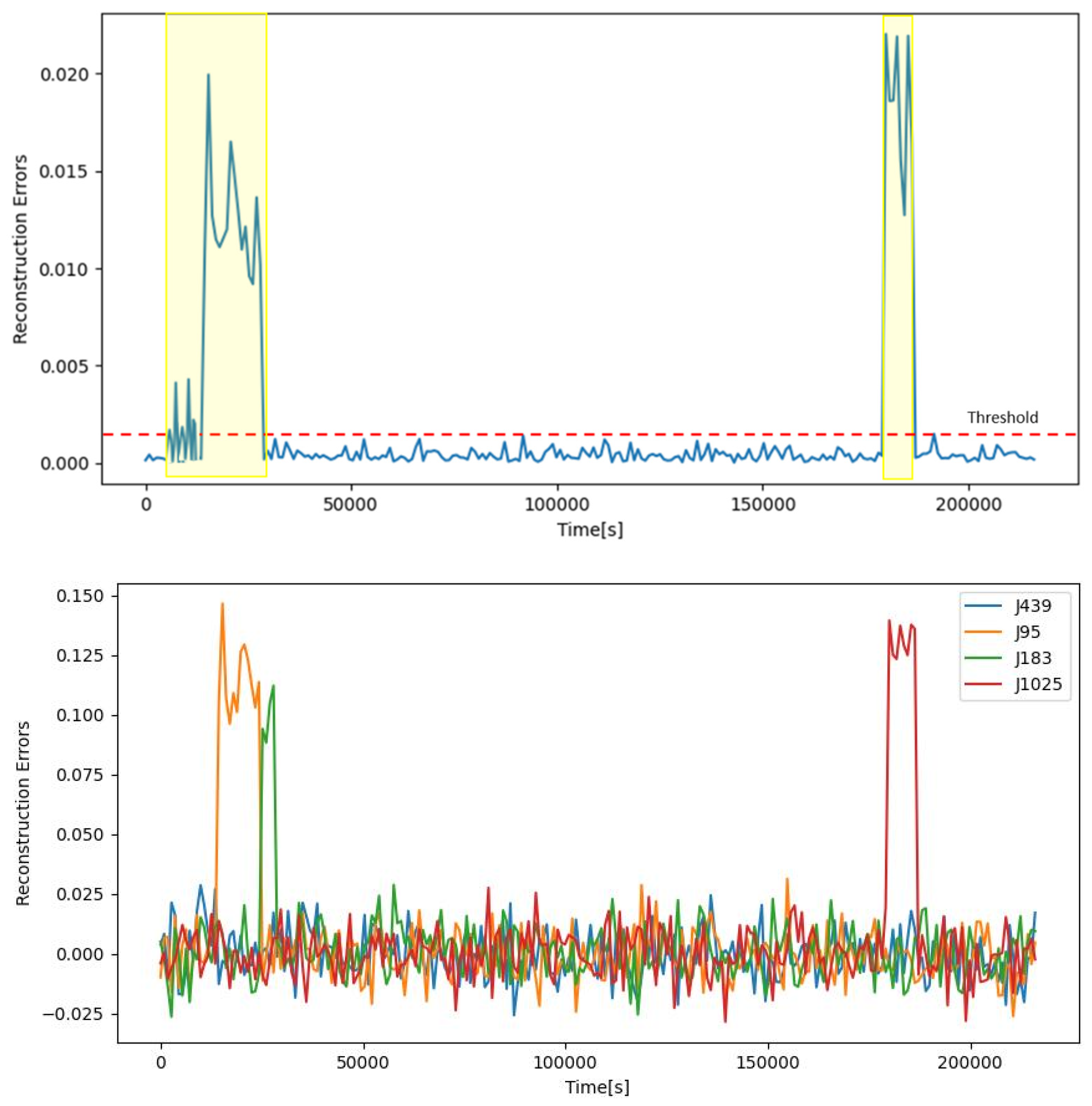
The second case study presented in the discussion highlights the effectiveness of the model in detecting and predicting leaks in the D-Town network. In this case, four leaks were registered in pipes ’J439’, ’J95’, ’J183’, and ’J1025’ over a period of 60 hours. These leaks occurred at different times and some of them overlapped.
Figure 9a illustrates the reconstruction and forecast errors of the model when applied to this test case. It is observed that the model performs well in detecting and predicting the leaks, as the errors are relatively small for most of the period. However, there are two noticeable periods where large errors are observed, namely from 2-8 hours and from 50-52 hours.
To further investigate the causes of these errors, Figure 9b provides an analysis. It is evident that the main causes of the errors are the pipes where the leaks occurred, namely ’J439’, ’J95’, ’J183’, and ’J1025’. This finding is expected, as these pipes were the ones where the leaks were registered.
Overall, this case study demonstrates the practical applicability of the model in real-world scenarios. The model successfully detects and predicts leaks in the network, with only a few instances of larger errors. This suggests that the model can be easily deployed and utilized to effectively manage and maintain water distribution networks, ultimately reducing water loss and improving overall system efficiency.
Figure 9.
Identified pipes leaks of different durations over a period of 60 hours, a) total reconstruction errors and b) individual errors.
Figure 9.
Identified pipes leaks of different durations over a period of 60 hours, a) total reconstruction errors and b) individual errors.
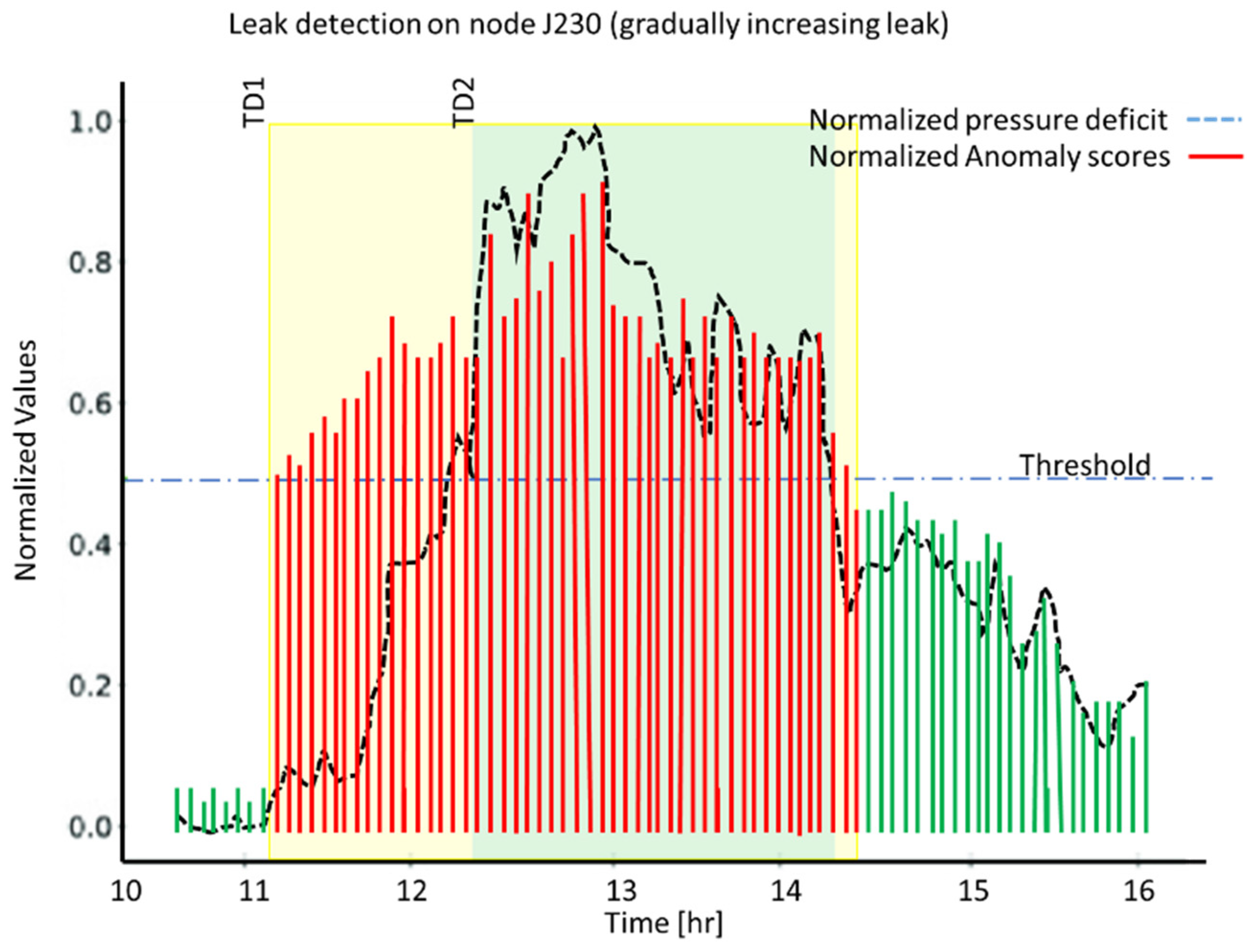
The detection time of the leak is a critical factor in leak management, as it directly impacts the efficiency and effectiveness of the response. By detecting the leak early, the necessary repairs can be carried out promptly, minimizing the impact on the water distribution system and reducing the potential for further damage or water loss. Therefore, the second case study was also used to analyze the detection time of the leaks. This is especially important for leaks which develop with time. A leak on node J230 resemble this feature and the results of detection are shown in Figure 10. This leak is of particular interest as it develops over time, making it crucial to detect it as early as possible to minimize water loss and potential damage.
The graph shows the detection time of the leak on node J230 over a period of 60 hours. It is observed that the proposed method successfully detects the leak at around 11.3 hours almost an hour earlier (TD1) than the simple pressure threshold method (TD2) and accurately predicts its duration. This early detection allows for prompt action to be taken to repair the leak and prevent further water loss.
Figure 10.
Leak detection of a gradually increasing leak using a pressure threshold method and our encoder method.
Figure 10.
Leak detection of a gradually increasing leak using a pressure threshold method and our encoder method.
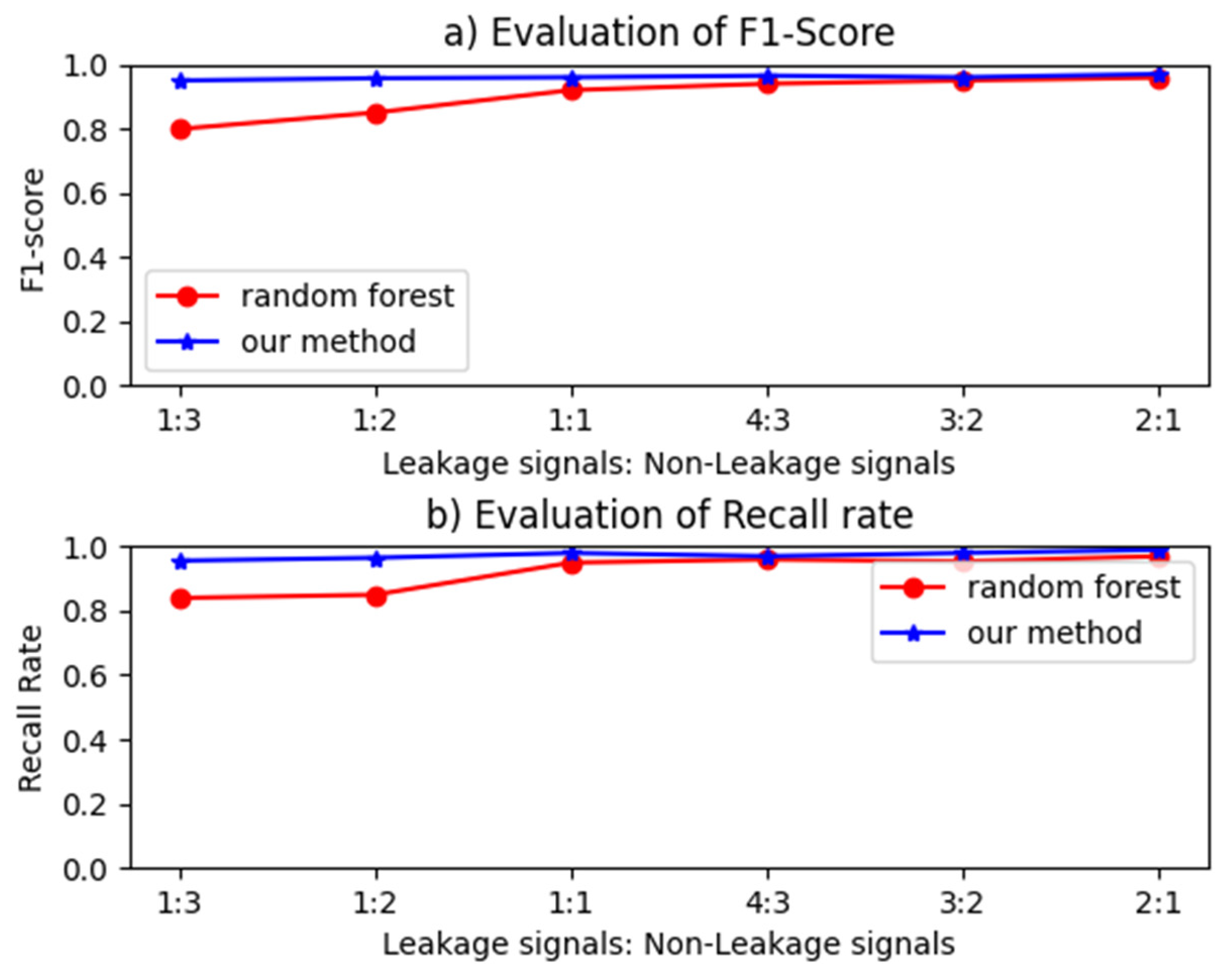
Furthermore, the principle of balanced class is fundamental in most machine learning models, as it ensures that all classes are given equal importance. However, unbalanced input data present a challenge as they can cause the models to overlook the minority classes. In the context of leak detection, the number of leakage signals is significantly lower than the number of non-leakage signals. To address this, the study analyzed the ratio of leakage to non-leakage signals in the training dataset and compared it to a random forest model based on supervised learning. The models were then trained and evaluated using different ratios, including 1:3, 1:2, 1:1, 4:3, 3:2, and 2:1. The evaluation results are depicted in Figure 11 for recall rate and F1-score. Both Figure 11a and Figure 11b demonstrate that the evaluation metrics of the machine learning models exhibit similar patterns as the proportion of data varies. Our method is hardly affected by the ratio of the leakage to non-leakage conditions. As for the supervised learning based random forest model, as the proportion approaches 1 to 4:3, the changes in the evaluation metrics become less pronounced. When the proportion of leakage to non-leakage signals is less than one, the recall rate and F1 value decrease rapidly, indicating a decline in the models’ classification performance. On the other hand, when the proportion exceeds 4:3, there is no significant improvement in the evaluation metrics as the ratio increases. However, it is important to note that collecting more leakage data would increase the cost of data acquisition. Therefore, this study chooses to train the random forest model with a proportion of one for the input data.
5. Discussion
Literature review have shown that leak detection in water distribution networks is a very challenging task with high demands on computation resources and real-time capability. The challenges are posed mainly by lack of monitoring data, noisy data, and intermittent water demand. Especially fluctuation in water demand make it very difficult for computer algorithms to differentiate between non-leaking and leaking conditions. Leak detection using inspection tools is very expensive and labor-intensive and cannot achieve real-time. The same applies to physical models which are difficult to implement for WSN due to complex topology and uncertainty in the hydraulic conditions and need domain expertise. Another approach which is quite common in literature is leak detection using transient responses. The problem with this method is that it requires to capture transient signals over a very short period when leak occurs, which requires high sampling rate. More promising this time of Artificial intelligence are Data-driven approaches using machine learning models. They can produce real-time and reliable leak detection. The rationale is that the spatial pattern of water pressure and its variations under leak are affected by the network structure of water distribution and should be considered in leak detection. The hybrid autoencoder model developed in this study takes both spatial and temporal information into consideration, allows to detect leak from unbalanced data, i.e., with only data under normal operational conditions and uses multiple nodes for detection. The method can provide near real-time leak detection with high accuracy and does not require strong domain expertise to implement. Unlike leak detection based on transient signals, which requires sensor with high sampling rates to capture the transient process. The AE leak detection model learn from the spatial pattern contained in the data and only needs sensor with low sampling rate. Furthermore, by using data from multiple nodes, the detection is more robust than data-driven models that only use data at single node.
While data used for model training and validation in this study are from generated data by high fidelity model for WSN. The framework is readily applied to real world data as could be shown in the second case study.
Here are some key findings and results from our study using 3DCNN ConvLSTM autoencoders for spatial-temporal pipe leak detection:
- Improved detection accuracy: The combination of 3DCNNs and ConvLSTMs has been found to improve the accuracy of leak detection compared to traditional methods. The network can effectively capture spatial features and temporal dynamics, enabling the detection of subtle changes in flow and pressure patterns caused by leaks.
- Early detection of leaks: The 3DCNN ConvLSTM autoencoder has shown the ability to detect leaks at an early stage, even before they become significant and easily detectable through traditional methods. This early detection can help prevent further damage and reduce water loss.
- Accurate leak localization: The network’s ability to capture spatial information allows for accurate leak localization. By comparing the input and output frames, the network can identify the specific pipes or areas where leaks are likely to be located. This enables targeted repair and maintenance actions, reducing the time and effort required for leak detection and repair.
- Robustness to noise and variations: The 3DCNN ConvLSTM autoencoder has demonstrated robustness to noise and variations in the data. It can handle fluctuations in flow rates, pressure levels, and other factors that may affect the accuracy of leak detection. This robustness improves the reliability of the system in real-world operating conditions.
- Generalizability across networks: The 3DCNN ConvLSTM autoencoder has been shown to be applicable to different types of water distribution networks, including networks with varying sizes, pipe materials, and topologies. This generalizability makes it a versatile approach that can be implemented in various contexts.
While the results of using 3DCNN ConvLSTM autoencoders for spatial-temporal pipe leak detection are promising, there are still some challenges and limitations. These include the need for large and diverse training datasets, the computational complexity of the network architecture, and the requirement for accurate and reliable sensor data.
Overall, the use of 3DCNN ConvLSTM autoencoders for spatial-temporal pipe leak detection in water distribution networks offers a data-driven approach that can improve the accuracy, early detection, and localization of leaks. Further research and development in this area can lead to more effective and efficient leak detection systems for sustainable water management.
6. Conclusions
Leak detection in water distribution networks is a necessary practice for water companies to minimize water loss and improve efficiency. The method proposed in the paper utilizes a hybrid framework of an autoencoder, which combines a 3D convolutional neural network (CNN) and a spatio-temporal decoder component called Convolutional Long Short-term Memory (ConvLSTM) network. The autoencoder network takes into account the spatial and temporal relationship of water pressure at multiple nodes in a water distribution network for leak detection. Spatial and temporal attention modules are incorporated in the model to improve the accuracy of both leak detection and localization. Data for the experiments is generated using the WNTR Simulator, which is based on the EPANET hydraulic model. The simulator includes pressure-driven demand nodes, allowing for the consideration of leaking conditions, fluctuating water demand, and data noise. The results of the leak detection experiments on the benchmark and real case studies demonstrate that the developed model is robust and capable of achieving high accuracy in detecting leaks.
7. Patents
There are no patents resulting from this manuscript.
Author Contributions
Divas Karimanzira is the sole author of this article.
Funding
This research received no external funding
Data Availability Statement
The data can be accessed upon request by the data providers. Other data we use in this study for example the D-Town WDN are all publicly available.
Acknowledgments
The author acknowledges everyone who was involved in any discussions in making the paper realizable. The author thank the editors and anonymous reviewers for their constructive comments that are greatly contributive to the revision of the manuscript.
Conflicts of Interest
The authors declare no conflict of interest.
References
- Kiliç, R. (2016). "Effective Management of Leakage in Drinking Water Network." Acta Physica Polonica, A. 130(1). [CrossRef]
- Fan, Xudong, Zhang, Xijin, Yu, Bill. (2021). Machine Learning Model and Strategy for Fast and Accurate Detection of Leaks in Water Supply Network. [CrossRef]
- Chan TK, Chin CS, Zhong X (2018) Review of current technologies and proposed intelligent methodologies for water distributed network leakage detection. IEEE Access 6:78846–78867. [CrossRef]
- Butler D (2000) Leakage detection and management: a comprehensive guide to technology and practice in the water supply industry. Palmer Environmental.
- Karney, Bryan and McInnis, Duncan. (1990). Transient Analysis of Water Distribution Systems. Journal - American Water Works Association. 82. 62-70. [CrossRef]
- Wang, Fang & Lin, Weiguo & Liu, Zheng & Qiu, Xianbo. (2019). Pipeline Leak Detection and Location Based on Model-Free Isolation of Abnormal Acoustic Signals. Energies. 12. 3172. [CrossRef]
- Colombo AF, Lee P, Karney BW (2009) A selective literature review of transient-based leak detection methods. J Hydro Environ Res 2(4):212–227. [CrossRef]
- Muhammad Aminuddin Pi, Remli, Mohd Fairusham Ghazali, W. H. Azmi , M. Y. Hanafi, Transient-Based Leak Detection and Monitoring of Water Pipes Using Complementary Ensemble Empirical Mode Decomposition (CEEMD) Method Journal of Advanced Research in Fluid Mechanics and Thermal Sciences Volume 83, Issue 2 (2021) 135-148.
- Simpson, A. R., & Wang, Z. (2009). Transient-based leak detection in water distribution pipes. Journal of Hydraulic Engineering, 135(9), 781-785.
- Karney, B. W. (2005). Leak detection in water distribution systems using transients. Journal of Water Resources Planning and Management, 131(2), 150-157.
- Bolognesi, A., & Alvisi, S. (2013). Leak detection in water distribution networks using transients: A review. Water, 5(4), 1951-1971.
- Barros, D.; Almeida, I.; Zanfei, A.; Meirelles, G.; Luvizotto, E., Jr.; Brentan, B. An Investigation on the Effect of Leakages on the Water Quality Parameters in Distribution Networks. Water 2023, 15, 324. [CrossRef]
- Zhao, H., & Simpson, A. R. (2017). Leak detection in water distribution pipes using wavelet analysis of transient signals. Journal of Hydroinformatics, 19(1), 1-14.
- Farley, M., & Simpson, A. R. (2011). Leak detection in water distribution pipes using the Hilbert-Huang transform. Journal of Hydraulic Engineering, 137(1), 89-97. doi:10.1061/(ASCE)HY.1943-7900.0000291 A.B.; Author 2, C.D. Title of the article. Abbreviated Journal Name Year, Volume, page range. [CrossRef]
- Srirangarajan S, Allen M, Preis A, Iqbal M, Lim HB, Whittle AJ (2013) Wavelet-based burst event detection and localization in water distribution systems. J Sign Proc Syst 72(1):1–16. [CrossRef]
- Moryan, Nathaniel C., "High Precision Pipeline Leak Detection and Localization Using Negative Pressure Wave Technique: An Application in a Real Field Case Study" (2022). Graduate Theses, Dissertations, and Problem Reports. 11479. https://researchrepository.wvu.edu/etd/11479.
- Adedeji KB, Hamam Y, Abe BT, Abu-Mahfouz AM (2017) Towards achieving a reliable leakage detection and localization algorithm for application in water piping networks: an overview. IEEE Access 5:20272–20285. [CrossRef]
- Neeraj*, Nawal, M., Bundele, M., & Suri, P. K. (2020). Leakage Detection through HL in Gurthali Water Supply Distribution Network using EPANET. In International Journal of Innovative Technology and Exploring Engineering (Vol. 9, Issue 3, pp. 3558–3565). Blue Eyes Intelligence Engineering and Sciences Engineering and Sciences Publication - BEIESP. [CrossRef]
- Soldevila, G. Boracchi, M. Roveri, S. Tornil-Sin and V. Puig. Leak detection and localization in water distribution networks by combining expert knowledge and data-driven models. Neural Computing and Applications, 34: 4759-4779, 2022. [CrossRef]
- Pal A, Kant K (2019) Water flow driven sensor networks for leakage and contamination monitoring in distribution pipelines. ACM Transact Sensor Netw (TOSN) 15(4):1–43. [CrossRef]
- Zhou X, Tang Z, Xu W, Meng F, Chu X, Xin K, Fu G (2019) Deep learning identifies accurate burst locations in water distribution networks. Water Res 166:115058. [CrossRef]
- Wu Y, Liu S (2017) A review of data-driven approaches for burst detection in water distribution systems. Urban Water J 14(9):972–983. [CrossRef]
- Chan TK, Chin CS, Zhong X (2018) Review of current technologies and proposed intelligent methodologies for water distributed network leakage detection. IEEE Access 6:78846–78867. [CrossRef]
- Bakker M, Vreeburg J et al (2013) A fully adaptive forecasting model for short-term drinking water demand. Environ Model Softw 48:141–151. [CrossRef]
- Mrchi et al , 2014.
- Walski, T., Blakley, D., Evans, M., and Whitman, B.: Verifying Pressure Dependent Demand Modeling, Proceed. Eng., 186, 364– 371, 2017. [CrossRef]
- Klise KA, Murray R et al (2018) An overview of the water network tool for resilience (WNTR). Sandia National lab. (SNL-NM), Albuquerque.
- Amran TST, Ismail MP et al (2017) Detection of underground water distribution piping system and leakages using ground penetrating radar (GPR). AIP Conference Proceedings, AIP Publishing LLC.
- van Zyl, Jakobus Ernst. "Theoretical modeling of pressure and leakage in water distribution systems." Procedia Engineering 89 (2014): 273-277.
- Funk A, De Oreo WB (2011) Embedded energy in water studies study 3: end-use water demand profiles. Prepared by Aquacraft, Inc. for the California Public Utilities Commission Energy Division, Managed by California Institute for Energy and Environment, CALMAC Study ID CPU0052.
- X. Shi, Z. Chen, H. Wang, D.-Y. Yeung, W. Wong, and W. Woo,‘‘Convolutional LSTM network: A machine learning approach for pre-cipitation nowcasting,’’ in Proc. Adv. Neural Inf. Process. Syst., 2015,pp. 802–810.
- Yao Tang, Lin Zhao, Shanshan Zhang, Chen Gong, Guangyu Li, Jian Yang, Integrating prediction and reconstruction for anomaly detection, Pattern Recognition Letters, Volume 129, 2020, Pages 123-130, ISSN 0167-8655. [CrossRef]
- Karimanzira, D. and Ritzau, L, Tobias Martin, and Thilo Fischer . (2023), “Advanced SpatioTemporal Event Detection System for Groundwater Quality Based on Deep Learning.” Applied Ecology and Environmental Sciences, vol. 11, no. 3 (2023): 79-90. [CrossRef]
- van Zyl, Jakobus E., and A. M. Cassa. "Modeling elastically deforming leaks in water distribution pipes." Journal of Hydraulic Engineering 140.2 (2014): 182-189.
Figure 1.
D-Town Water distribution network showing the pipelines and the demand nodes.
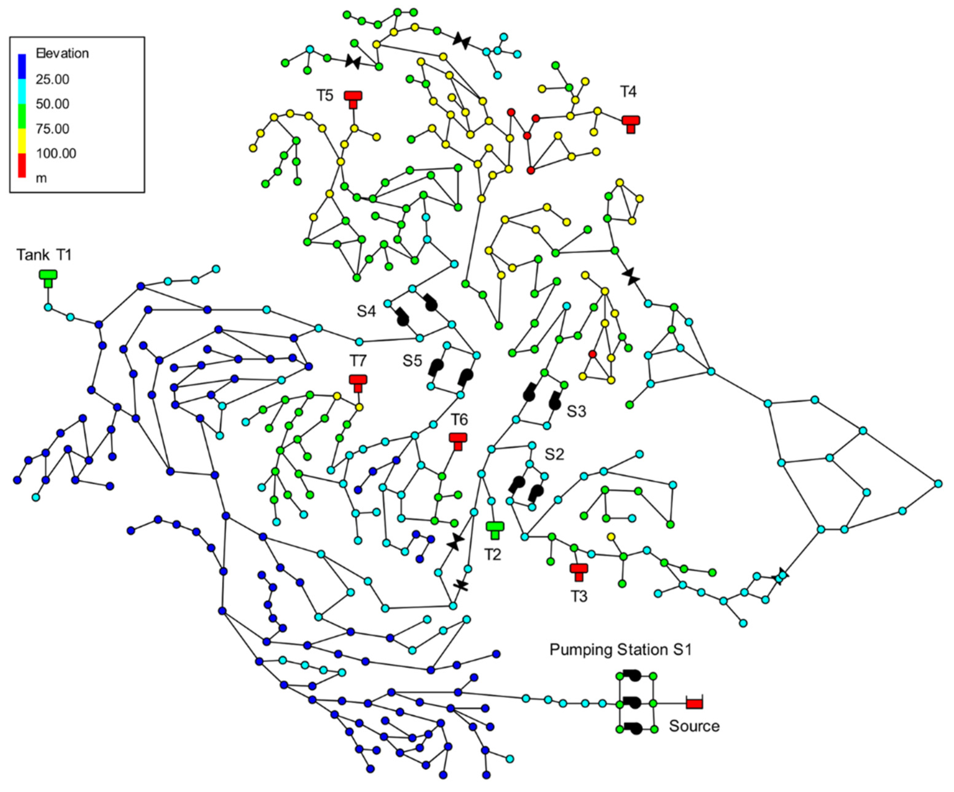
Figure 2.
3-dimensional multivariate spatio-temporal data used by the 3DCNN encoder.
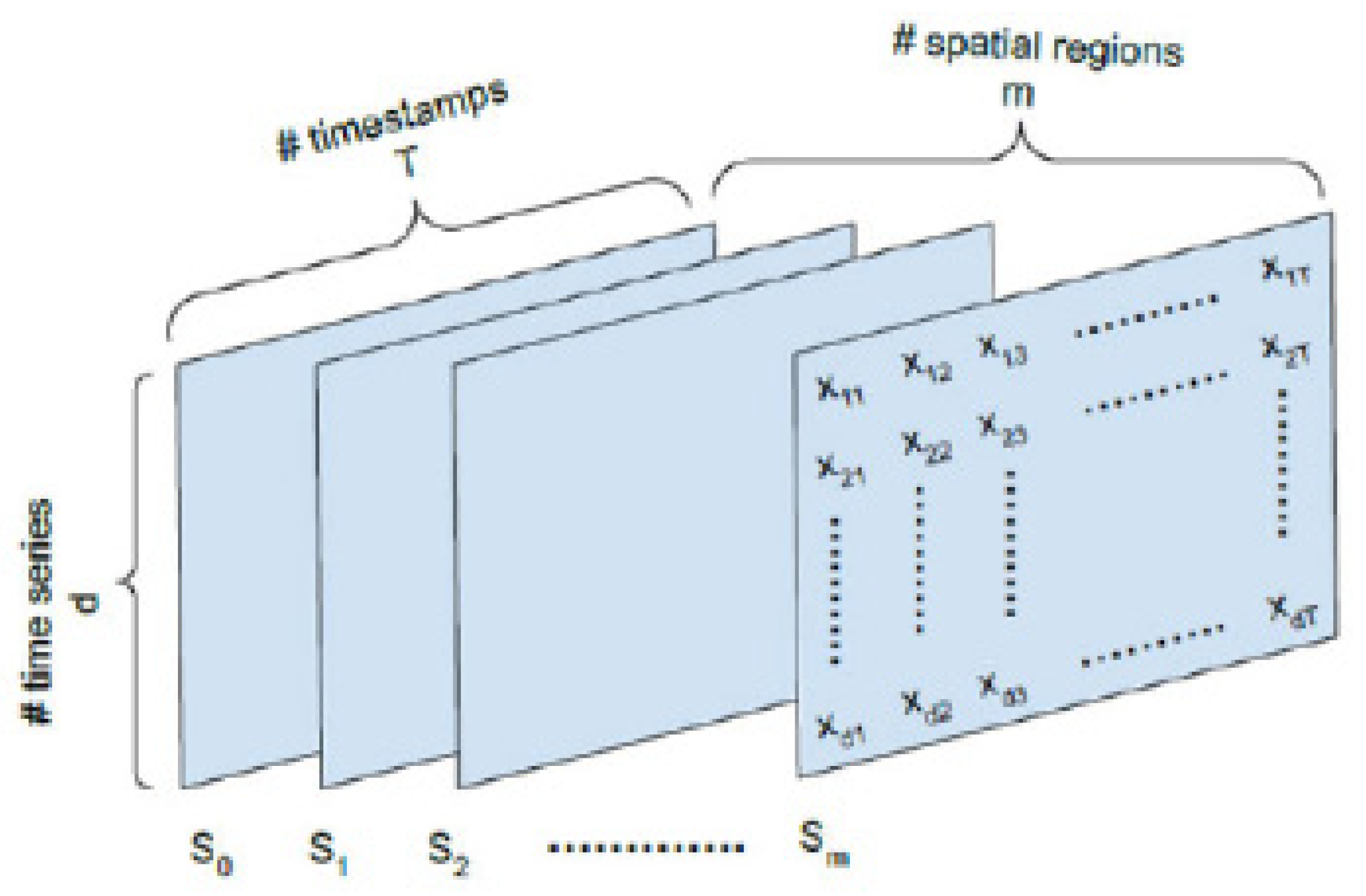
Figure 4.
Model results, Histogram of the reconstruction error for data under normal non-leaking condition versus leaking situation.
Figure 4.
Model results, Histogram of the reconstruction error for data under normal non-leaking condition versus leaking situation.
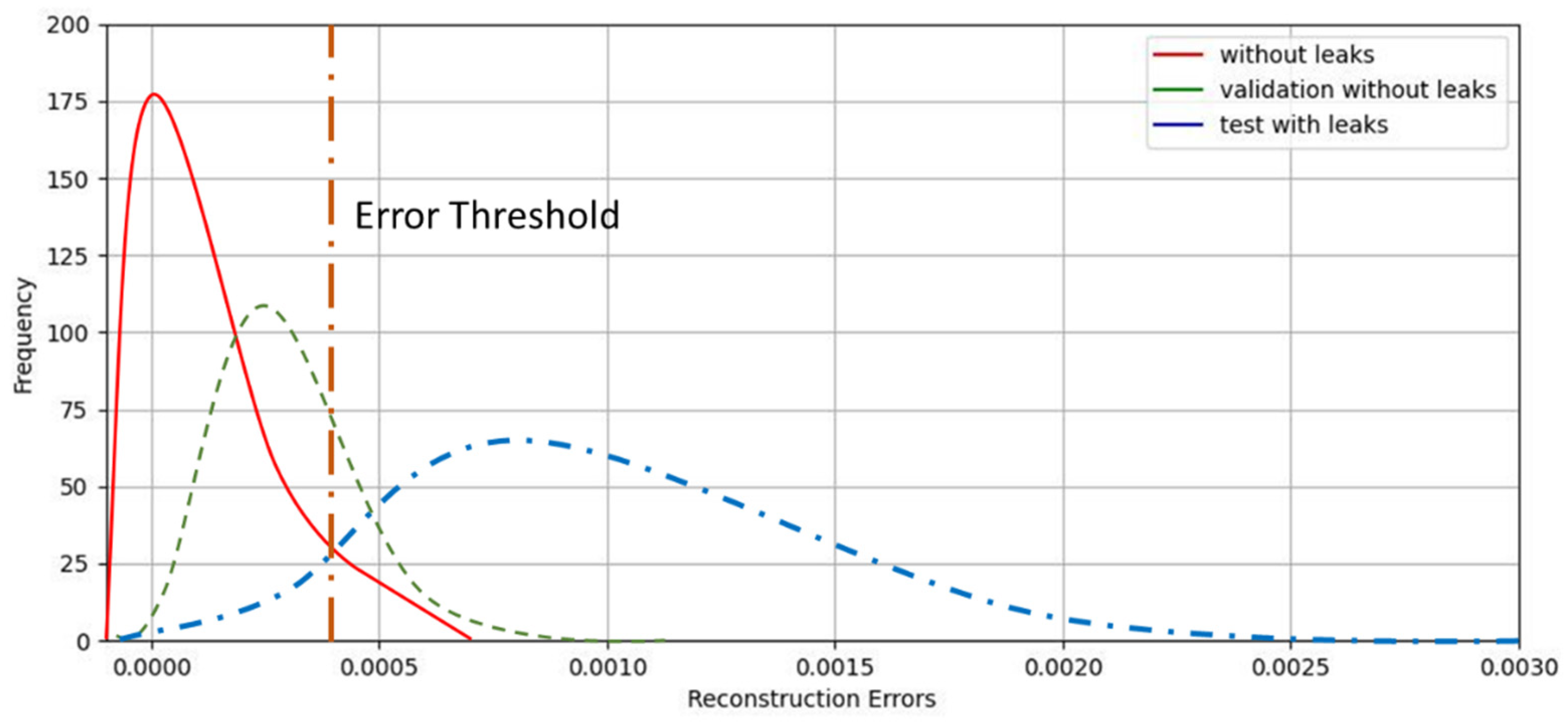
Figure 5.
Leaks with different characteristic over a period of 1 week.
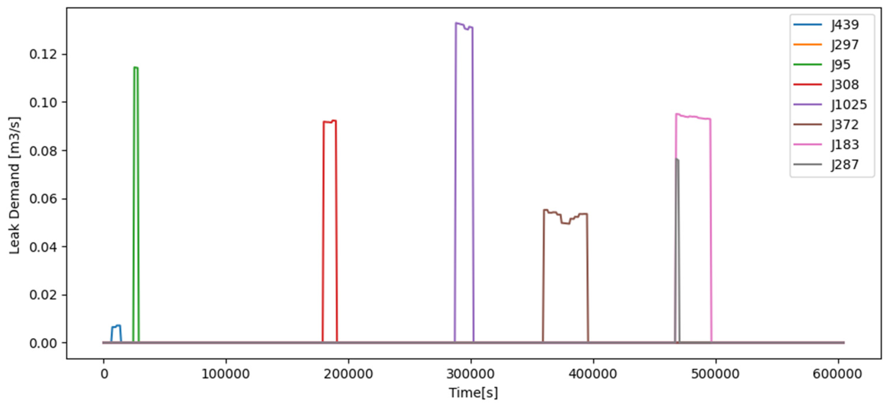
Figure 11.
Effect of different ratios on the identification results of our model and a random forest model based on supervised learning. a) recall rate and b) F1-score.
Figure 11.
Effect of different ratios on the identification results of our model and a random forest model based on supervised learning. a) recall rate and b) F1-score.
Disclaimer/Publisher’s Note: The statements, opinions and data contained in all publications are solely those of the individual author(s) and contributor(s) and not of MDPI and/or the editor(s). MDPI and/or the editor(s) disclaim responsibility for any injury to people or property resulting from any ideas, methods, instructions or products referred to in the content. |
© 2023 by the authors. Licensee MDPI, Basel, Switzerland. This article is an open access article distributed under the terms and conditions of the Creative Commons Attribution (CC BY) license (http://creativecommons.org/licenses/by/4.0/).
Copyright: This open access article is published under a Creative Commons CC BY 4.0 license, which permit the free download, distribution, and reuse, provided that the author and preprint are cited in any reuse.


